Optimal Estimation of Large Functional and Longitudinal Data by Using Functional Linear Mixed Model

Abstract

The estimation of large functional and longitudinal data, which refers to the estimation of mean function, estimation of covariance function, and prediction of individual trajectory, is one of the most challenging problems in the field of high-dimensional statistics. Functional Principal Components Analysis (FPCA) and Functional Linear Mixed Model (FLMM) are two major statistical tools used to address the estimation of large functional and longitudinal data; however, the former suffers from a dramatically increasing computational burden while the latter does not have clear asymptotic properties. In this paper, we propose a computationally effective estimator of large functional and longitudinal data within the framework of FLMM, in which all the parameters can be automatically estimated. Under certain regularity assumptions, we prove that the mean function estimation and individual trajectory prediction reach the minimax lower bounds of all nonparametric estimations. Through numerous simulations and real data analysis, we show that our new estimator outperforms the traditional FPCA in terms of mean function estimation, individual trajectory prediction, variance estimation, covariance function estimation, and computational effectiveness.

1. Introduction

Functional Data Analysis (FDA) is a field of statistics that examines data to provide information about curves, surfaces, or anything else that varies along a continuum [1]. The concrete continuum of these functions can be time, spatial location, wavelength, and probability, with applications to biomechanics, biomedicine, ecology, epidemiology, and neurology, among many others [2,3]. Functional data can be classified into common design data and independent design data, where the sampling locations of all individuals are the same under the former setting, while the sampling locations are individual-wise under the latter setting [4]. Longitudinal data can be regarded as a specific type of functional data where the underlying continuum is just time [5]. In the field of longitudinal data analysis, the counterparts of common design and independent design are called balanced longitudinal data and unbalanced longitudinal data, respectively.

The coronavirus 2019 (COVID-19) data is typical balanced longitudinal data, which records the daily infections (transformed in logarithm) of the COVID-19 pandemic from 51 states of the United States (US), where the date is from 16 March 2020 to 14 August 2020 (Johns Hopkins COVID-19 Case Tracker: https://www.kaggle.com/datasets/thecansin/johns-hopkins-covid19-case-tracker?resource=download). Figure 1 demonstrates the profiles of daily increasing infections and the related trajectories predictions separately yielded with the R package mgcv [6] of six states in the US. From this figure, it is easy to see some basic features of large longitudinal data: (1) functionality, the daily infections of states are likely some smooth curves of time; (2) heterogeneity, different individuals usually have different trends over time; and (3) high-dimensionality, the number of observations ($T=152$) much larger than the number of individuals ($N=51$). How to deal with this kind of large functional and longitudinal data is one of the most challenging problems in the field of high-dimensional statistics.

Functional Principal Components Analysis (FPCA) and Functional Linear Mixed Model (FLMM) are two common approaches that estimate the dominant modes of variation of a sample of random trajectories around an overall mean function. FPCA and FLMM share the same principle to estimate the mean function, but apply totally different strategies to estimate the covariance function and predict the individual trajectory. Specifically, FPCA first estimates the two-dimensional covariance function, then yields the eigenfunctions through PCA, and finally predicts the individual trajectory with the estimated eigenfunctions. In contrast, FLMM parameterizes the individual trajectories through basis functions, in particular, it specifies a Gaussian prior distribution on the coefficients of basis functions, then estimates the covariance matrix of these random coefficients using REstricted Maximum Likelihood (REML) [7], and eventually predicts the individual trajectories through the Best Linear Unbiased Prediction (BLUP) [8] and yields the covariance function of random curves using a weighted sum of inner products of basis functions. Commonly-employed nonparametric techniques for FPCA include the kernel method and local polynomial modeling ([9,10,11] and smoothing splines ([12,13,14,15,16]), while frequently-used basis expansion functions include B-splines ([17,18,19,20]), wavelets ([21,22,23]), a combination of linear mixed-effects modeling and local polynomial smoothing ([24,25]), etc. See more aspects of functional data in the following monographs ([1,26]) and review papers ([3,27,28]).

One of the greatest advantages of FPCA may be its clear asymptotic properties. Under mild regularity conditions, Yao et al. [11] showed the convergence rates of estimates of mean function covariance function, variance, eigenfunctions, and eigenvalues. Li and Hsing [10] further derived the strong uniform convergence rates of these estimates. Cai and Yuan [4] investigated the minimax risks of the mean function and covariance function estimates and Cai and Yuan [29] showed the minimax risk of mean function estimate in functional linear regression. However, because FPCA needs to estimate a two-dimensional covariance surface, its computational burden will dramatically increase as the number of observations T rises. In addition, since most FPCA methods employ local polynomial modeling [30] as the estimator, it is very difficult to select the optimal bandwidth in the two-dimensional kernel function in practice. On the other hand, FLMM suffers from more problems compared with FPCA, preventing its practical application in the field of FDA. First, FLMM requires estimating the covariance matrix of the basis expansion coefficients (which are treated as normal variables in LMM), but the estimation of this covariance matrix is usually unreliable if the number of employed bases is large. James et al. [17] provided a dimension reduction to estimate this covariance matrix, which resulted in a more complex estimator. Besides, the asymptotic properties of FLMM are difficult to study. Proper regularity conditions and proof techniques are lacking for FLMM.

In this paper, we propose a computationally effective estimator of large functional and longitudinal data by using FLMM, in which all the parameters can be automatically estimated. We also investigate the large sample property of the proposed automatic and flexible estimation of large functional data. Under mild regularity conditions, we prove that the estimation error of the mean curve estimator is bounded by $O(N^{-1}+T^{-2s})$ and the prediction error of the individual trajectory estimator is bounded by $O\left(T^{-2s/(2s+1)}\right)$, where $s>1$ is a constant governing the smoothness of tge mean function and individual trajectory. In particular, both these two convergence rates reach the minimax lower boundaries of the mean function estimation and individual trajectory prediction derived by Cai and Yuan [4], meaning that our estimation enjoys the minimax efficiency. To the best of our knowledge, our work is the first to investigate the large sample property of FLMM estimation when both T and N are diverging.

The rest of the paper is organized as follows. In Section 2, we present the primal representation of FLMM to analyze the functional data. In Section 3, the new estimator of large balanced longitudinal data and its large sample property are illustrated. In Section 4, we exhibit the simulation studies. In Section 5, we apply our method to study the COVID-19 data. The concluding remarks are summarized in Section 6 and all the technical proofs of the theorems are relegated to the Appendix.

2. Preliminary

In this section, we introduce the functional data and the top two statistical methods, i.e., FPCA and FLMM, to deal with the functional data briefly.

2.1. Settings

For a vector $\mathit{a}={\left(a_j\right)}_{p\times 1}$, ${\left|\right|\mathit{a}\left|\right|}_q=({\sum }_{j=1}^p|a_j{{|}^q)}^{1/q}$ with $q\in [0,\infty ]$. For a symmetric matrix $\mathbf{A}={\left(A_{ij}\right)}_{p\times p}$, ${\lambda }_{max}\left(\mathbf{A}\right)$ and ${\lambda }_{min}\left(\mathbf{A}\right)$ denote the maximum and minimum eigenvalues of matrix $\mathbf{A}$, and ${\left|\right|\mathbf{A}\left|\right|}_q={max\left\{\right|\left|\mathbf{A}\mathit{a}\right||}_q{,\left|\right|\mathit{a}\left|\right|}_q=1\}$. Besides, $a_n\asymp b_n$ if there are positive constants c and C such that $c\le a_n/b_n\le C$. In addition, $O(·)$ and $o(·)$ are the infinitely large and small quantities, respectively, while $O_P(·)$ and $o_P(·)$ mean that such relationships hold with a probability tending to 1.

2.2. Functional Data Model

Let $X\left(t\right)$ be a second-order stochastic process defined in the compact interval $\mathcal{T}$, which is usually set as $\mathcal{T}=[0,1]$ for convenience. The covariance function of $X\left(t\right)$ is given by

$$\begin{array}{c}\hfill C(s,t)=\mathrm{E}\left[\right\{X\left(s\right)-\mathrm{E}\left(X\right(s\left)\right)\left\}\right\{X\left(t\right)-\mathrm{E}\left(X\right(t\left)\right)\left\}\right],(s,t)\in \mathcal{T}\times \mathcal{T}.\end{array}$$

(1)

Besides, let $X_1\left(t\right),\cdots ,X_N\left(t\right)$ be N independent realizations of $X\left(t\right)$, $\{t_1,\dots ,t_T\}$ be T sampling locations of the realizations, and the observations of $X_i\left(t_j\right)$ be

$$\begin{array}{c}\hfill Y_{ij}=X_i\left(t_j\right)+{\epsilon }_{ij},(i,j)\in \{1,\dots ,N\}\times \{1,\dots ,T\},\end{array}$$

(2)

where ${\epsilon }_{ij}$ are independent and identically distributed (IID) random errors with mean 0 and variance ${\sigma }^2$. In addition, the sampling location is considered as fixed numbers in $\mathcal{T}$, and $\left\{X_i\left(t_j\right)\right\}$ and $\left\{e_{ij}\right\}$ are two mutually independent groups. In a more general case, the sampling locations can vary from individual, i.e.,

$$\begin{array}{c}\hfill Y_{ij}=X_i\left(t_{ij}\right)+{\epsilon }_{ij},(i,j)\in \{1,\dots ,N\}\times \{1,\dots ,T_i\},\end{array}$$

(3)

where $t_{ij}$ is a random sampling location and $T_i$ is the individual-wise sampling locations. In the literature, the setting of functional data subject to (2) is called common design, while the setting subject to (3) is termed independent design. In longitudinal data analysis where t is just time, the data subject to (2) is named as balanced longitudinal data or panel data, while the data subject to (3) is named as the unbalanced longitudinal data.

2.3. Methodologies of FPCA and FLMM

FPCA is almost the most frequently used technique to deal with the functional data in which the Karhunen–Loève representation of the stochastic process plays a central role. Specifically, let covariance function $C(s,t)$ satisfy the definition of a Mercer kernel, i.e.,

$$\begin{array}{c}\hfill \sum _{i=1}^n\sum _{j=1}^{n}C(s_i,t_j)c_i{c}_j\ge 0\end{array}$$

(4)

for all finite sequence of points $(s_i,t_j)\in \mathcal{T}\times \mathcal{T}$ and all choices of real numbers $c_1,\dots ,c_n$. Then, according to Mercer’s theorem, there consequently exists a series of eigenfunctions $\left\{{\varphi }_k\left(t\right)\right\}$ and a series of non-increasing eigenvalues $\left\{{\lambda }_k\right\}$ satisfying ${\sum }_{k=1}^{\infty }{\lambda }_k<\infty$ such that

$$\begin{array}{c}\hfill C(s,t)=\sum _{k=1}^{\infty }{\lambda }_k{\varphi }_k\left(t\right){\varphi }_k\left(s\right),(s,t)\in \mathcal{T}\times \mathcal{T}.\end{array}$$

(5)

In particular, under the condition of Mercer kernel, the Karhunen–Loève representation theory is able to guarantee that the ith realization of $X\left(t\right)$ can be expressed as

$$\begin{array}{c}\hfill X_i\left(t\right)=\mu \left(t\right)+\sum _{k=1}^{\infty }{\xi }_{ik}{\varphi }_k\left(t\right),t\in \mathcal{T},\end{array}$$

(6)

where $\mu \left(t\right)$ is termed the mean function and ${\xi }_{i1},\dots ,{\xi }_{ik},\dots$ are uncorrelated random coordinates with mean 0 and variance E$\left({\xi }_{ik}^2\right)={\lambda }_k$.

FLMM deals with the functional data in a more direct way than FPCA. Specifically, FLMM expresses each random function by some known basis functions:

$$\begin{array}{c}\hfill X_i\left(t\right)=\sum _{k=1}^p{\mathsf{\Psi }}_k\left(t\right)b_{ik}+{\delta }_i\left(t\right),\end{array}$$

(7)

where $\left\{{\mathsf{\Psi }}_k\left(t\right)\right\}$ are a set of basis functions, $\left\{b_{ik}\right\}$ are the corresponding random coordinates, and ${\delta }_i\left(t\right)$ is the approximation bias. In practice, the basis functions can be the Tikhonov basis (as defined in $\mathcal{T}=[0,1]$):

$$\begin{array}{c}\hfill {\mathsf{\Psi }}_k\left(t\right)=\sqrt{2}cos\left((k-1)\pi t\right).\end{array}$$

(8)

Alternatively, B-splines [31] are common bases that are generated in an iterative procedure. If ${\delta }_i\left(t\right)$ is negligible, the uncertainty of random function $X_i\left(t\right)$ is almost described by the random coordinates $\left\{b_{ik}\right\}$. In the literature, it is routine to assume

$$\begin{array}{c}\hfill \left(\begin{array}{c}{b}_{i1}\\ b_{i2}\\ ⋮\\ b_{ip}\end{array}\right)\sim \mathcal{N}\left(\begin{array}{c}\left(\begin{array}{c}{\mathit{\beta }}_1\\ {\mathit{\beta }}_2\\ ⋮\\ {\mathit{\beta }}_p\end{array}\right),\left(\begin{array}{cccc}{\mathsf{\Gamma }}_{11}& {\mathsf{\Gamma }}_{12}& \cdots & {\mathsf{\Gamma }}_{1p}\\ {\mathsf{\Gamma }}_{21}& {\mathsf{\Gamma }}_{22}& \cdots & {\mathsf{\Gamma }}_{2p}\\ ⋮& ⋮& \ddots & ⋮\\ {\mathsf{\Gamma }}_{p1}& {\mathsf{\Gamma }}_{p2}& \cdots & {\mathsf{\Gamma }}_{pp}\end{array}\right)\end{array}\right),\end{array}$$

(9)

where ${\beta }_1,\dots ,{\beta }_p$ are the mean parameters and $\mathbf{\Gamma }={\left({\mathsf{\Gamma }}_{ij}\right)}_{p\times p}$ is a covariance matrix. As a result,

$$\begin{array}{c}\hfill \mu \left(t\right)\approx \sum _{k=1}^p{\mathsf{\Psi }}_k\left(t\right){\beta }_k,C(s,t)\approx \sum _{k=1}^p\sum _{h=1}^p{\mathsf{\Gamma }}_{kh}{\mathsf{\Psi }}_k\left(s\right){\mathsf{\Psi }}_h\left(t\right).\end{array}$$

(10)

In addition, if $\left\{{\mathsf{\Psi }}_k\left(t\right)\right\}$ are chosen as the eigenfunctions of the covariance function $C(s,t)$, the covariance matrix $\mathbf{\Gamma }$ will reduce into a diagonal matrix with the eigenvalues $\left\{{\lambda }_k\right\}$. On the other hand, FPCA can reduce to an FLMM if the eigenfunctions are rotated for a better practical interpretation, which is subject to a similar idea of factor analysis [32]. Generally, since $C(s,t)$ is never known in advance, FLMM will employ certain commonly-used basis functions and estimate $\mathbf{\Gamma }$ empirically.

2.4. Comparison between FPCA and FLMM

FLMM is more efficient than FPCA in terms of both estimation and prediction. Due to the space limitation, we directly give the conclusions and show the estimation procedures of FPCA and FLMM in Appendix B.

We illustrate the features of FPCA from two aspects: estimation and prediction. For estimation, FLMM does not require estimating a two-dimensional covariance surface $C(s,t)$, which is the most time-consuming component for FPCA. Besides, all terms in FLMM can be automatically estimated using many mature and effective algorithms, such as the Newton–Raphson algorithm. Whereas the main approaches for FPCA to estimate the mean $\mu \left(t\right)$ and covariance $C(s,t)$ are local linear modeling [10], which is based on the Kernel function, it requires determining three different bandwidths $h_u,h_C,h_v$ (see details in Appendix B), which is supposedly very complex in practice. For prediction, FPCA will use all the observations in addition to the local linear coefficients ${\widehat{a}}_0,\dots ,{\widehat{c}}_1$, which are generated in the estimation process, to predict the values of $\mu \left(t\right)$, $X_{i^{*}}\left(t\right)$, $C(s,t)$ at any new locations $t_{i^{*}j}$ (and $s_{i^{*}j}$), which is extremely costly in implementation. In contrast, predicting these functions is trivial for FLMM: it only needs to generate a new vector ${\mathbf{\Psi }}_{i^{*}}={(\mathsf{\Psi }\left(t_{i^{*}1}\right),\dots ,\mathsf{\Psi }\left(t_{i^{*}{T}_{i^{*}}}\right))}^{\top }$ and then predict the values by using $\widehat{\mathit{\beta }}$, ${\widehat{\mathit{b}}}_i$, $\widehat{\mathbf{\Gamma }}$ and ${\widehat{\sigma }}^2$.

However, the most serious problem of FLMM is the lack of statistical theory in comparison with the numerous theoretical investigations of FPCA. One theoretical burden of FLMM is inherited from the LMM and generalized linear model (GLM, [33]): the statistical properties of LMM and GLM are different to analyze. As far as we are concerned, the tool to investigate the asymptotic properties of GLM is first given by Vonesh et al. [34], who pointed out that the convergence rate of the mean parameter is of $O\left(T_{min}^{-1/2}\right)$, where $T_{min}$ is the minimum number of observations among all individuals. However, this convergence rate is not ideal because $T_{min}$ can be less than 10 in many longitudinal data. Many works aim to improve the GLM estimation by removing the high-order bias of Laplace approximation, such as [35,36,37]; however, these bias-corrections make the asymptotic properties more difficult to analyze.

Another theoretical burden of FLMM is inherited from the basis expansion method, approximating a smooth function through a series of basis functions. As Ruppert et al. [38] once commented: “The literature on inference in smoothing is large and varied. Much of it is in the local polynomial or kernel smoothing context, where theoretical properties are more tractable. Inference for spline-based smoothing is less studied.” Indeed, it is unclear under what conditions the FLMM using the basis expansion method is consistent. In the next section, we improve the traditional FLMM in terms of these two burdens.

3. Optimal Estimation for Large Balanced Longitudinal Data

In this paper, we propose a novel FLMM estimation for large balanced longitudinal data, which is effective in terms of computation and optimal in terms of statistical theory. Our new FLMM estimation for large balanced longitudinal data is motivated by the COVID-19 data, in which the number of sampling locations (i.e., the dates from 16 March 2020 to 14 August 2020) is much larger than the number of individuals (i.e., the 50 states plus the District of Columbia). The traditional estimation of FLMM may encounter numerical instability and becomes extremely time-consuming because the complexity of the REML estimator dramatically increases with the dimension of the covariance matrix ${\mathbf{\Sigma }}_y$. In contrast, our new estimator for the variance components remains efficient and stable even when the dimension of ${\mathbf{\Sigma }}_y$ is very high. Note that under the setting of balanced longitudinal data, the sampling locations are the same for all individuals, i.e., $\mathit{t}={(t_1,\dots ,t_T)}^{\top }$, the covariance matrix ${\mathbf{\Sigma }}_{y_i}$ will become a universal one ${\mathbf{\Sigma }}_y$ and the basis function matrix ${\mathbf{\Psi }}_i$ will reduce to a universal matrix $\mathbf{\Psi }$ for all individuals.

3.1. Novel Estimating Procedure

The biggest difference between our new estimation and the traditional one is that we will use different numbers of basis functions to estimate the mean function and the individual trajectory. In order to guarantee both the mean function estimation and individual trajectory prediction meet the optimal convergence rates, we approximate the mean function and individual trajectory as follows. Specifically:

$$\begin{array}{c}\hfill \mu \left(t\right)\approx \sum _{k=1}^q{\mathsf{\Psi }}_k\left(t\right){\beta }_k,X_i\left(t\right)\approx \mu \left(t\right)+\sum _{k=1}^p{\mathsf{\Psi }}_k\left(t\right)c_{ik},\end{array}$$

(11)

where $1\le p\le q\le T$. Regarding the matrix form, we have

$$\begin{array}{c}\hfill \mathit{\mu }\approx {\mathbf{\Psi }}_q\mathit{\beta },{\mathit{X}}_i\approx \mathit{\mu }+{\mathsf{\Psi }}_p{\mathit{c}}_i,\end{array}$$

(12)

where ${\mathbf{\Psi }}_q={\left({\mathsf{\Psi }}_k\left(t_j\right)\right)}_{T\times q}$, ${\mathbf{\Psi }}_p={\left({\mathsf{\Psi }}_k\left(t_j\right)\right)}_{T\times p}$, $\mathit{\beta }={({\beta }_1,\dots ,{\beta }_q)}^{\top }$, ${\mathit{c}}_i={(c_{i1},\dots ,c_{ip})}^{\top }$. Here, the vector of random coordinates ${\mathit{c}}_i$ is considered to follow a normal distribution

$$\begin{array}{c}\hfill {\mathit{c}}_i\sim \mathcal{N}(\mathbf{0},\mathbf{\Gamma }),\end{array}$$

(13)

where $\mathbf{\Gamma }=\left({\mathsf{\Gamma }}_{jk}\right)$ is a $(p\times p)$ positive definite symmetric matrix. It is used to describe the local variability of individual trajectory $X_i\left(t\right)$ beyond the mean function $\mu \left(t\right).$

The first step of our estimator is estimating the mean coefficient $\mathit{\beta }$:

$$\begin{array}{cc}\hfill \widehat{\mathit{\beta }}& =arg\underset{\mathit{\beta }}{min}\left\{\sum _{i=1}^N{({\mathit{Y}}_i-{\mathbf{\Psi }}_q\mathit{\beta })}^{\top }{\widehat{\mathbf{\Sigma }}}_y^{-1}({\mathit{Y}}_i-{\mathbf{\Psi }}_q\mathit{\beta })+\gamma {\mathit{\beta }}^{\top }\mathbf{Q}\mathit{\beta }\right\}\hfill \\ \hfill & ={(N{\mathbf{\Psi }}_q^{\top }{\widehat{\mathbf{\Sigma }}}_y^{-1}{\mathbf{\Psi }}_q+\gamma \mathbf{Q})}^{-1}{\mathbf{\Psi }}_q^{\top }{\widehat{\mathbf{\Sigma }}}_y^{-1}\left(\sum _{i=1}^N{\mathit{Y}}_i\right),\hfill \end{array}$$

(14)

where ${\widehat{\mathbf{\Sigma }}}_y={\widehat{\sigma }}^2{\mathbf{I}}_T+{\mathbf{\Psi }}_p\widehat{\mathbf{\Gamma }}{\mathbf{\Psi }}_p^{\top }$, $\gamma$ is a smoothing parameter, and $\mathbf{Q}$ is a known semi-positive definite symmetric matrix ensuring

$$\begin{array}{c}\hfill {\int }_{t\in \mathcal{T}}{\left[{\mu }^{{}^{″}}\left(t\right)\right]}^{2}dt\approx {\mathit{\beta }}^{\top }\mathbf{Q}\mathit{\beta }.\end{array}$$

(15)

Compared with traditional FLMM, which estimates $\mu \left(t\right)$ by (A51), we add a ridge penalty ${\mathit{\beta }}^{\top }\mathbf{Q}\mathit{\beta }$ to control the smoothness of $\mathit{\mu }\left(t\right)$. If $\mathsf{\Psi }\left(t\right)$ is chosen as the Tikhonov bases, then $\mathbf{Q}$ is a diagonal matrix with the jth entry $P_{jj}=2{\left((j-1)\pi \right)}^4$. If $\mathsf{\Psi }\left(t\right)$ is chosen as the Bsplines, then $\mathbf{Q}={\mathbf{D}}_2^{\top }{\mathbf{D}}_2$ where the expression of ${\mathbf{D}}_2$ can be found in Eilers and Marx [31]. In addition, the covariance matrix of $\widehat{\mathit{\beta }}$ is given by

$$\begin{array}{c}\hfill \mathrm{cov}\left(\widehat{\mathit{\beta }}\right)={(N{\mathbf{\Psi }}_q^{\top }{\widehat{\mathbf{\Sigma }}}_y^{-1}{\mathbf{\Psi }}_q+\gamma \mathbf{Q})}^{-1}.\end{array}$$

(16)

When T is large, we recommend the Sherman–Morrison–Woodbury formula to yield ${\widehat{\mathbf{\Sigma }}}_y^{-1}$:

$$\begin{array}{c}\hfill {\widehat{\mathbf{\Sigma }}}_y^{-1}=\frac{1}{{\widehat{\sigma }}^2}\left({\mathbf{I}}_T-{\mathbf{\Psi }}_p{({\mathbf{\Psi }}_p^{\top }{\mathbf{\Psi }}_p+{\widehat{\sigma }}^2{\widehat{\mathbf{\Gamma }}}^{-1})}^{-1}{\mathbf{\Psi }}_p^{\top }\right).\end{array}$$

(17)

The mean function is then given by $\widehat{\mathit{\mu }}={\mathbf{\Psi }}_q\widehat{\mathit{\beta }}$ and its asymptotic covariance matrix is

$$\begin{array}{c}\hfill \mathrm{cov}\left(\widehat{\mathit{\mu }}\right)={\mathbf{\Psi }}_q{(N{\mathbf{\Psi }}_q^{\top }{\widehat{\mathbf{\Sigma }}}_y^{-1}{\mathbf{\Psi }}_q+\gamma \mathbf{Q})}^{-1}{\mathbf{\Psi }}_q^{\top }.\end{array}$$

(18)

The confidence band of $\widehat{\mathit{\mu }}$ is constructed by using the diagonal elements of $\mathrm{cov}\left(\widehat{\mathit{\mu }}\right)$.

The second step is to predict ${\mathit{c}}_i$ by using BLUP:

$$\begin{array}{cc}\hfill \widehat{{\mathit{c}}_i}& =arg\underset{{\mathit{c}}_i}{min}\{\frac{1}{{\widehat{\sigma }}^2}\left|\right|{\mathit{Y}}_i-\widehat{\mathit{\mu }}-{\mathbf{\Psi }}_p{\mathit{c}}_i{\left|\right|}_2^2+{\mathit{c}}_i^{\top }{\widehat{\mathbf{\Gamma }}}^{-1}{\mathit{c}}_i\}\hfill \\ \hfill & =({\mathbf{\Psi }}_p^{\top }{\mathbf{\Psi }}_p+{\widehat{\sigma }}^2{\widehat{\mathbf{\Gamma }}}^{-1}){\mathbf{\Psi }}_p^{\top }({\mathit{Y}}_i-\widehat{\mathit{u}}).\hfill \end{array}$$

(19)

This estimator is called BLUP because $\widehat{{\mathit{c}}_i}$ can be regarded as the mean of the posterior distribution of ${\mathit{c}}_i$. The prediction of ${\mathit{X}}_i$ is ${\widehat{\mathit{X}}}_i=\widehat{\mathit{\mu }}+\mathbf{\Psi }{\widehat{\mathit{c}}}_i$. In addition, the asymptotic covariance matrix of ${\widehat{\mathit{c}}}_i$ is

$$\begin{array}{c}\hfill \mathrm{cov}\left({\widehat{\mathit{c}}}_i\right)={\widehat{\sigma }}^2{({\mathbf{\Psi }}_p^{\top }{\mathbf{\Psi }}_p+{\widehat{\sigma }}^2{\widehat{\mathbf{\Gamma }}}^{-1})}^{-1},\end{array}$$

(20)

and the asymptotic covariance matrix of ${\widehat{\mathit{X}}}_i$ is given by

$$\begin{array}{c}\hfill \mathrm{cov}\left({\widehat{\mathit{X}}}_i\right)={\mathbf{\Psi }}_q{(N{\mathbf{\Psi }}_q^{\top }{\widehat{\mathbf{\Sigma }}}_y^{-1}{\mathbf{\Psi }}_q+\gamma \mathbf{Q})}^{-1}{\mathbf{\Psi }}_q^{\top }+{\widehat{\sigma }}^2{\mathbf{\Psi }}_p{({\mathbf{\Psi }}_p^{\top }{\mathbf{\Psi }}_p+{\widehat{\sigma }}^2{\widehat{\mathbf{\Gamma }}}^{-1})}^{-1}{\mathsf{\Psi }}_p^{\top },\end{array}$$

(21)

which is used to constructed the confidence band of ${\widehat{\mathit{X}}}_i$.

The novelty of our new estimating procedure is the estimator of $\mathbf{\Gamma }$ and ${\sigma }^2$. Specifically, our method employs the Laplace Approximation Marginal Likelihood (LAML) [39] to estimate $\mathbf{\Gamma }$ and ${\sigma }^2$, which has a much lower computational cost than REML. The objective function of $\mathbf{\Gamma }$ and ${\sigma }^2$ based on LAML is given by

$$\begin{array}{cc}\hfill \mathcal{L}({\sigma }^2,\mathbf{\Gamma })=& \sum _{i=1}^N\left\{\frac{1}{{\widehat{\sigma }}^2}\left|\right|{\mathit{Y}}_i-\widehat{\mathit{\mu }}-{\mathbf{\Psi }}_p{\widehat{\mathit{c}}}_i{\left|\right|}_2^2+{\widehat{\mathit{c}}}_j^{\top }{\mathbf{\Gamma }}^{-1}{\widehat{\mathit{c}}}_j+logdet{\mathbf{\Gamma }}^{-1}+log\left({\sigma }^2{\mathbf{I}}_T\right)\right\}\hfill \\ \hfill & +logdet\left(\frac{{\mathbf{\Psi }}_p^{\top }{\mathbf{\Psi }}_p}{{\sigma }^2}+{\mathbf{\Gamma }}^{-1}\right).\hfill \end{array}$$

(22)

In this objective function, the first four components come from the joint log-likelihood function of $\left\{{\mathit{Y}}_i\right\}$ and $\left\{{\mathit{c}}_i\right\}$, while the fifth term is resulted by the Laplace approximation of integral $\int f\left({\mathit{Y}}_i\right|{\mathit{c}}_i)f\left({\mathit{c}}_i\right)d{\mathit{c}}_i$, where $f\left({\mathit{Y}}_i\right|{\mathit{c}}_i)$ is the density function of ${\mathit{Y}}_i$ conditioned on ${\mathit{c}}_i$ and $f\left({\mathit{c}}_i\right)$ is the density function of ${\mathit{c}}_i$. The derivative of $\mathcal{L}({\sigma }^2,\mathbf{\Gamma })$ with respective to ${\sigma }^{-2}$ is

$$\begin{array}{c}\hfill \frac{\partial \mathcal{L}({\sigma }^2,\mathbf{\Gamma })}{\partial {\sigma }^{-2}}=\mathbf{0}=-NT{\sigma }^2+\sum _{i=1}^N\left(\left|\right|{\mathit{Y}}_i-\widehat{\mathit{\mu }}-{\mathbf{\Psi }}_p{\widehat{\mathit{c}}}_i{\left|\right|}_2^2\right)+\mathrm{trace}(\Delta ({\sigma }^2,\mathbf{\Gamma }){\mathbf{\Psi }}_p^{\top }{\mathbf{\Psi }}_p),\end{array}$$

(23)

where $\Delta ({\sigma }^2,\mathbf{\Gamma })={({\mathbf{\Psi }}_p^{\top }{\mathbf{\Psi }}_p/{\sigma }^2+{\mathbf{\Gamma }}^{-1})}^{-1}$. As a result, the fixed-point iteration for ${\sigma }^2$ is

$$\begin{array}{c}\hfill {\sigma }^{2[t+1]}=\frac{1}{NT}\left\{\sum _{i=1}^N\left(\left|\right|{\mathit{Y}}_i-\widehat{\mathit{\mu }}-{\mathbf{\Psi }}_p{\widehat{\mathit{c}}}_i{\left|\right|}_2^2\right)+\mathrm{trace}(\Delta ({\sigma }^{2\left[t\right]},{\mathbf{\Gamma }}^{\left[t\right]}){\mathbf{\Psi }}_p^{\top }{\mathbf{\Psi }}_p)\right\},\end{array}$$

(24)

where ${\sigma }^{2\left[t\right]}$ and ${\mathbf{\Gamma }}^{\left[t\right]}$ are the current estimates. On the other hand, the derivative of $\mathcal{L}({\sigma }^2,\mathbf{\Gamma })$ with respective to ${\mathbf{\Gamma }}^{-1}$ is

$$\begin{array}{c}\hfill \frac{\partial \mathcal{L}({\sigma }^2,\mathbf{\Gamma })}{\partial {\mathbf{\Gamma }}^{-1}}=-N\mathbf{\Gamma }+\sum _{i=1}^N\left({\widehat{\mathit{c}}}_i{\widehat{\mathit{c}}}_i^{\top }\right)+\Delta ({\sigma }^2,\mathbf{\Gamma }).\end{array}$$

(25)

Hence, the fixed-point iteration for $\mathbf{\Gamma }$ is

$$\begin{array}{c}\hfill {\mathbf{\Gamma }}^{[t+1]}=\frac{1}{N}\left\{\sum _{i=1}^N\left({\widehat{\mathit{c}}}_i{\widehat{\mathit{c}}}_i^{\top }\right)+\Delta ({\sigma }^{2\left[t\right]},{\mathbf{\Gamma }}^{\left[t\right]})\right\}.\end{array}$$

(26)

We implement these two fixed-point iterations iteratively and regard the stable solutions as ${\widehat{\sigma }}^2$ and $\widehat{\mathbf{\Gamma }}$. Likewise, we also implement the estimator of $\mathit{\beta }$, the predictors of $\left\{{\mathit{c}}_i\right\}$, and the estimator of $\mathbf{\Gamma }$ and ${\sigma }^2$ iteratively, and regard the stable solutions as the outputting estimates of $\mathit{\beta }$, $\left\{{\mathit{c}}_i\right\}$, $\mathbf{\Gamma }$, and ${\sigma }^2$.

The reason why LAML is more efficient than REML is illustrated as follows. The objective function of REML with respect to balanced longitudinal data is

$$\begin{array}{c}\hfill \mathcal{R}\left(\mathit{\vartheta }\right)=\sum _{i=1}^N\left({({\mathit{Y}}_i-{\mathbf{\Psi }}_q\widehat{\mathit{\beta }})}^{\top }{\mathbf{\Sigma }}_y^{-1}({\mathit{Y}}_i-{\mathbf{\Psi }}_q\widehat{\mathit{\beta }})+logdet\left({\mathbf{\Sigma }}_y\right)\right)+logdet\left({\mathbf{\Psi }}_q^{\top }{\mathbf{\Sigma }}_y^{-1}{\mathbf{\Psi }}_q\right),\end{array}$$

(27)

where $\mathit{\vartheta }=({\sigma }^2,\mathrm{vec}\left(\mathbf{\Gamma }\right))$ and ${\mathbf{\Sigma }}_y\approx {\sigma }^2{\mathbf{I}}_T+{\mathbf{\Psi }}_p\mathbf{\Gamma }{\mathbf{\Psi }}_p^{\top }$. Because ${\sigma }^2$ and $\mathbf{\Gamma }$ are involved in ${\mathbf{\Sigma }}_y$, it is impossible to obtain fixed-point iterations for ${\sigma }^2$ and $\mathbf{\Gamma }$ separately as LAML. In other words, it seems that the only way to jointly estimate ${\sigma }^2$ and vec($\mathbf{\Gamma }$) is by using the Fisher-scoring algorithm. The first-order derivative of $\mathcal{R}\left(\mathit{\vartheta }\right)$ with respect to ${\vartheta }_k$ is

$$\begin{array}{c}\hfill \frac{\partial \mathcal{R}\left(\mathit{\vartheta }\right)}{\partial {\vartheta }_k}=0=-\sum _{i=1}^N{({\mathit{Y}}_i-{\mathbf{\Psi }}_q\widehat{\mathit{\beta }})}^{\top }{\mathbf{\Sigma }}_y^{-1}\frac{\partial {\mathbf{\Sigma }}_y}{\partial {\vartheta }_k}{\mathbf{\Sigma }}_y^{-1}({\mathit{Y}}_i-{\mathbf{\Psi }}_q\widehat{\mathit{\beta }})+\mathrm{trace}\left(\mathbf{P}\frac{\partial {\mathbf{\Sigma }}_y}{\partial {\vartheta }_k}\right),\end{array}$$

(28)

while the expectation of second-order derivative of $\mathcal{R}\left(\mathit{\vartheta }\right)$ with respect to ${\vartheta }_k$ and ${\vartheta }_h$, i.e., the ($k,h$)th element of the Hessian matrix of $\mathcal{R}\left(\mathit{\vartheta }\right)$, is given by

$$\begin{array}{c}\hfill \mathrm{E}\left(\frac{{\partial }^2\mathcal{R}\left(\mathit{\vartheta }\right)}{\partial {\vartheta }_k\partial {\vartheta }_h}\right)=\mathrm{trace}\left(\mathbf{P}\frac{\partial {\mathbf{\Sigma }}_y}{\partial {\vartheta }_k}\mathbf{P}\frac{\partial {\mathbf{\Sigma }}_y}{\partial {\vartheta }_h}\right),\end{array}$$

(29)

where

$$\begin{array}{c}\hfill \mathbf{P}={\mathbf{\Sigma }}_y^{-1}-{\mathbf{\Sigma }}_y^{-1}{\mathbf{\Psi }}_q{\left({\mathbf{\Psi }}_q^{\top }{\mathbf{\Sigma }}_y^{-1}{\mathbf{\Psi }}_q\right)}^{-1}{\mathbf{\Psi }}_q^{\top }{\mathbf{\Sigma }}_y^{-1}.\end{array}$$

(30)

Thus, $\mathit{\vartheta }$ is updated by

$$\begin{array}{c}\hfill {\mathit{\vartheta }}^{[t+1]}={\mathit{\vartheta }}^{\left[t\right]}-\mathbf{H}{\left({\mathit{\vartheta }}^{\left[t\right]}\right)}^{-1}\mathit{g}\left({\mathit{\vartheta }}^{\left[t\right]}\right),\end{array}$$

(31)

where the kth element of $\mathit{g}\left({\mathit{\vartheta }}^{\left[t\right]}\right)$ is calculated according to (28) and the ($k,h$)th element of $\mathbf{H}\left({\mathit{\vartheta }}^{\left[t\right]}\right)$ is yielded by (29).

It is worth pointing out that there is no matrix formula to directly yield $\mathit{g}\left({\mathit{\vartheta }}^{\left[t\right]}\right)$ and $\mathbf{H}\left({\mathit{\vartheta }}^{\left[t\right]}\right)$, i.e., it is the sole way to calculate their elements one-by-one according to (28) and (29). This drawback makes the minimization of REML extremely costly because the computation complexity of matrix inverse ${\mathbf{\Sigma }}_y^{-1}$ and matrix product $\mathbf{P}\partial {\mathbf{\Sigma }}_y/\partial {\mathit{\vartheta }}_k$ are of $O\left(T^3\right)$. In particular, as the number of employed basis function p increases, the number of elements in $\mathbf{H}\left({\mathit{\vartheta }}^{\left[t\right]}\right)$ is ${(p^2+1)}^2$, which will be more than $10,000$ if p is just 10. As a result, the total computation complexity of the Hessian matrix calculation is $O\left(T^3{p}^4\right)$, which is unacceptable for large balanced longitudinal data. In contrast, our separate fixed-point iterations (24) and (26) have only $O\left(T{p}^2\right)$ computation complexity, and are able to guarantee ${\widehat{\sigma }}^2$ positive and $\widehat{\mathbf{\Gamma }}$ positive definite as long as the initial estimates ${\sigma }^{2\left[0\right]}$ is positive and ${\mathbf{\Gamma }}^{\left[0\right]}$ is positive definite. Therefore, our novel estimator is more attractive than the REML-based one for FLMM in high dimensionality. Note that what we contribute is the fixed-point iterations based on LAML. In the paper of LAML [39], the Newton–Raphson algorithm was employed to minimize the corresponding LAML objective function, in which will still face the same numerical problems as REML if T or p is large.

3.2. Regularity Assumptions

Now we turn to investigate the large sample properties of FLMM using our novel estimator. We first give three essential concepts that play central roles in our asymptotic investigation.

Definition 1 

(Sub-Gaussianity). A random error ${\epsilon }_i$ with mean $\mathrm{E}\left({\epsilon }_i\right)=0$ and variance $\mathit{var}\left({\epsilon }_i\right)={\sigma }^2$ is termed a sub-Gaussian variable if for all $r\in \mathrm{R}$,

$$\mathrm{E}(exp\left(r{\epsilon }_i\right))\le exp\left(\frac{1}{2}{\tau }^2{r}^2\right),$$

where $\tau >0$ is called the sub-Gaussian parameter.

Definition 2 

(Well-conditioned covariance matrix). An $(p\times p)$ symmetric matrix Σ is termed the well-conditioned covariance matrix if there is a constant $c_0$ independent of p such that

$$0<c_0^{-1}\le {\lambda }_{min}\left(\mathbf{\Sigma }\right)\le {\lambda }_{max}\left(\mathbf{\Sigma }\right)\le c_0<\infty .$$

Definition 3 

(Sobolev–Hilbert space). A functional space ${\mathcal{F}}_s$ is called s-order Sobolev–Hilbert space if there is a constant $c_0$ such that $\forall f\in {\mathcal{F}}_s$,

$$\mathrm{E}\left({\int }_{t\in \mathcal{T}}{\left[f^s\left(t\right)\right]}^{2}dt\right)\le c_0<\infty .$$

Sub-Gaussianity is an important concept in high-dimensional statistical analysis, which generalizes the Gaussian distribution to include common continuous variables and all bounded discrete variables [40]. Besides, the concept of well-conditioned covariance is proposed by Bickel and Levina [41], which guarantees that all of its eigenvalues are bounded away from zero and infinity whatever its dimension is. In addition, Sobolev–Hilbert space is the most commonly-used functional space in nonparametric statistical analysis [42]. The minimax lower bound of function estimate in this space is

$$\begin{array}{c}\hfill \underset{\widehat{f}}{inf}\underset{f\in {\mathcal{F}}_s}{sup}\mathrm{E}\left(\right||\widehat{f}-{f\left|\right|}_2^2)\ge d_0{N}^{-\frac{2s}{2s+1}},\end{array}$$

(32)

where $d_0>0$ is a certain constant and N describes the sample size.

Now we give the following assumptions that facilitate the proofs of theorems.

Assumption 1 

(Sub-Gaussian random error). For all $(i,j)\in \{1,\dots ,N\}\times \{1,\dots ,T\}$, the random error ${\epsilon }_{ij}$ is independently and identically distributively generated from a sub-Gaussian distribution with mean 0, variance ${\sigma }^2$, and sub-Gaussian parameter ${\tau }_{ϵ}$.

Assumption 2 

(Quasi uniform locations). The sampling locations $t_1,\dots ,t_T$ form a quasi uniform sequence defined in $\mathcal{T}$.

Assumption 3 

(Basis functions). For a series of basis functions $\left\{{\mathbf{\Psi }}_k\left(t\right)\right\}$,

$${\int }_{t\in \mathcal{T}}{\mathbf{\Psi }}_k\left(t\right)d_t=0,{\int }_{t\in \mathcal{T}}{\left[{\mathbf{\Psi }}_k\left(t\right)\right]}^{2}dt=1,{\int }_{t\in \mathcal{T}}{\left[{\mathbf{\Psi }}_k\left(t\right)\right]}^{4}dt\le c_0<\infty ,$$

for all $k\in \{1,\dots ,p\}$, where $c_0>0$ is a constant. Besides, let ${\mathbf{\Psi }}_p\left(t\right)={({\mathbf{\Psi }}_1\left(t\right),\dots ,{\mathbf{\Psi }}_p\left(t\right))}^{\top }$ and

$${\mathbf{\Sigma }}_{{\mathbf{\Psi }}_p}={\int }_{t\in \mathcal{T}}{\mathbf{\Psi }}_p\left(t\right){\mathbf{\Psi }}_p{\left(t\right)}^{\top }dt.$$

Then ${\mathbf{\Sigma }}_{{\mathbf{\Psi }}_p}$ is a well-conditioned covariance matrix.

Assumption 4 

(Approximation error of mean function). For a mean function $\mu \left(t\right)\in {\mathcal{F}}_s$ and a series of basis functions $\left\{{\mathsf{\Psi }}_k\left(t\right)\right\}$ satisfying Assumption 3, there exists a unique series of coefficients $\left\{{\beta }_k\right\}$ satisfying ${lim}_{q\to \infty }{\sum }_{k=1}^q{\beta }_k^2\le c_0<\infty$ such that

$${\int }_{t\in \mathcal{T}}{\left(\mu \left(t\right)-\sum _{k=1}^q{\mathsf{\Psi }}_k\left(t\right){\beta }_k\right)}^{2}dt\le c_0{q}^{-2s},$$

where $c_0>0$ is certain constant.

Assumption 5 

(Approximation error of individual function). For any individual trajectory $X_i\left(t\right)\in {\mathcal{F}}_s$ and a series of basis functions $\left\{{\mathsf{\Psi }}_k\left(t\right)\right\}$ satisfying Assumption 3, there exists a unique series of random coefficients $\left\{c_{ik}\right\}$ satisfying ${lim}_{p\to \infty }{\sum }_{k=1}^{p}E\left(c_{ik}^2\right)\le c_0<\infty$ such that

$$E\left({\int }_{t\in \mathcal{T}}{\left[X_i\left(t\right)-\mu \left(t\right)-\sum _{k=1}^p{\mathsf{\Psi }}_k\left(t\right)c_{ik}\right]}^{2}dt\right)\le c_0{p}^{-2s},i\in \{1,\dots ,N\},$$

where $c_0>0$ is certain constant.

Assumption 6 

(Distribution of random coefficients). Random coefficient $c_{ik}$ is sub-Gaussian with E$\left(c_{ik}\right)=0$, var($c_{ik})={\mathsf{\Gamma }}_{kk}$, sub-Gaussian parameter ${\tau }_k$, and $c_{ik}$ is independent of $c_{jk}$ for all $i\ne j$. Furthermore, $T\mathbf{\Gamma }={\left(T{\mathsf{\Gamma }}_{jk}\right)}_{p\times p}$ is a well-conditioned covariance matrix.

Assumption 1 considers the random error to be independent and identically distributed (IID) sub-Gaussian variable for all i and j. Assumption 2 sets the sampling locations and $t_1,\dots ,t_T$ can be regarded as a uniform sequence. As a result, the related integral of a certain function of t can be approximated by averaging the values of this function at these discrete locations. Assumption 3 summarizes some basic properties of the basis functions $\left\{{\mathsf{\Psi }}_k\left(t\right)\right\}$. Assumptions 4 and 5 describe how the accuracy of a function can be approximated by using p bases. Tsybakov [43] showed that, if the bases are the Tikhonov bases, Assumptions 4 and 5 hold as long as $\mu \left(t\right)$ and $X_i\left(t\right)$ belong to the Sobolev–Hilbert space ${\mathcal{F}}_s$. However, for a series of general basis functions, it remains unclear if Assumptions 4 and 5 still hold. In other words, we assume that we have picked the basis functions that have similar properties as the Tikhonov bases such that these two hold. Assumption 6 lists some conditions of the random coefficients. In particular, since

$$\begin{array}{c}\hfill {\lambda }_{max}\left(\mathbf{\Psi }\mathbf{\Gamma }{\mathbf{\Psi }}^{\top }\right)=O_P\left(T\right)\times {\lambda }_{max}\left({\mathbf{\Sigma }}_{\mathsf{\Psi }}\right)\times {\lambda }_{max}\left(\mathbf{\Gamma }\right),\end{array}$$

(33)

${\lambda }_{max}\left(\mathbf{\Gamma }\right)$ must be $O\left(T^{-1}\right)$ otherwise the covariance matrix of ${\mathbf{Y}}_i$ becomes divergent and violates some basic assumption of FDA; see, e.g., assumption (A4) in Yao et al. [11]. Hence, we assume that the covariance matrix of $\sqrt{T}{\mathit{c}}_i$, i.e., $T\mathbf{\Gamma }$, is well-conditioned.

3.3. Large Sample Property

We provide four theorems describing the asymptotic properties of estimators obtained by our new FLMM.

Theorem 1. 

Suppose Assumptions 1–6 hold. If $\widehat{\mathit{\beta }}$ is yielded by (14), ${\lambda }_{max}\left(\gamma \mathbf{Q}\right)=O\left(1\right)$, and ${\widehat{\mathbf{\Sigma }}}_y$ is chosen such that ${\lambda }_{max}\left({\widehat{\mathbf{\Sigma }}}_y^{-1}{\mathbf{\Sigma }}_y\right)\le c_0<\infty$ for certain constant $c_0>0$, then

$$\left|\right|\widehat{\mathit{\beta }}-\mathit{\beta }{\left|\right|}_2^2=O_P\left(\frac{q}{NT}+\frac{1}{q^{2s}}\right).$$

If $q=O\left(T\right)$, then the optimal convergence rate of $\widehat{\mathit{\beta }}$ is

$$\left|\right|\widehat{\mathit{\beta }}-\mathit{\beta }{\left|\right|}_2^2=O_P\left(\frac{1}{N}+\frac{1}{T^{2s}}\right).$$

Theorem 1 indicates the convergence rate of the mean parameter estimate $\widehat{\mathit{\beta }}$, which is a trade-off between variance term $O_P(q/NT)$ and bias term $O\left(p^{-2s}\right)$. As a corollary,

$$\begin{array}{cc}\hfill {\int }_{t\in \mathcal{T}}{(\mu \left(t\right)-\widehat{\mu }\left(t\right))}^{2}dt& \le {\int }_{t\in \mathcal{T}}{(\mu \left(t\right)-{\mathbf{\Psi }}_q{\left(t\right)}^{\top }\mathit{\beta })}^{2}dt+\frac{1}{T}\sum _{j=1}^T{\left({\mathbf{\Psi }}_q{\left(t_j\right)}^{\top }\{\mathit{\beta }-\widehat{\mathit{\beta }}\}\right)}^2\hfill \\ \hfill & =O_P\left(\frac{q}{NT}+\frac{1}{q^{2s}}\right).\hfill \end{array}$$

(34)

which means that the optimal convergence rate $\widehat{\mu }\left(t\right)$ is $O_P(N^{-1}+T^{-2s})$ by letting $q=O\left(T\right)$. In particular, this convergence rate reaches the minimax lower bound of all nonparametric estimates of $\mu \left(t\right)$ [29,43], indicating that our estimate is optimal in terms of minimax efficiency. Besides, our theory does not require $\lambda$ to vanish asymptotically. Indeed, any $\gamma$ such that ${\lambda }_{max}\left(\gamma \mathbf{Q}\right)=O\left(1\right)$ is able to guarantee $\widehat{\mathit{\beta }}$ to reach the minimax lower bound.

Theorem 2. 

Suppose Assumptions 1–6 hold. If ${\widehat{\mathit{c}}}_i$ is yielded by (19), then for $i=1,\dots ,N$,

$$\left|\right|{\widehat{\mathit{c}}}_i-{\mathit{c}}_i{\left|\right|}_2^2=O_P\left(\frac{p}{T}+\frac{1}{p^{2s}}\right).$$

If $p=O\left(T^{\frac{1}{2s+1}}\right)$, then the optimal convergence rate of ${\widehat{\mathit{c}}}_i$ is

$$\left|\right|{\widehat{\mathit{c}}}_i-{\mathit{c}}_i{\left|\right|}_2^2=O_P\left(T^{-\frac{2s}{2s+1}}\right).$$

Theorem 2 shows the convergence rate of the parameter estimate in individual trajectory ${\widehat{\mathit{c}}}_i$, which is a trade-off between variance term $O_P(p/T)$ and bias term $O\left(p^{-2s}\right)$. Similarly, the optimal convergence rate of ${\widehat{X}}_i\left(t\right)$ is

$$\begin{array}{cc}\hfill {\int }_{t\in \mathcal{T}}{(X_i\left(t\right)-{\widehat{X}}_i\left(t\right))}^{2}dt& \le {\int }_{t\in \mathcal{T}}{(X_i\left(t\right)-\mu \left(t\right)-{\mathbf{\Psi }}_p{\left(t\right)}^{\top }{\mathit{c}}_i)}^{2}dt+{\int }_{t\in \mathcal{T}}{(\mu \left(t\right)-\widehat{\mu }\left(t\right))}^{2}dt\hfill \\ \hfill & +\frac{1}{T}\sum _{j=1}^T{\left({\mathbf{\Psi }}_p{\left(t_j\right)}^{\top }\{{\mathit{c}}_i-{\widehat{\mathit{c}}}_i\}\right)}^2=O_P\left(\frac{p}{T}+\frac{1}{p^{2s}}\right),\hfill \end{array}$$

(35)

which reaches the minimax lower bound of all nonparametric estimates of $X_i\left(t\right)$ [29,43] by letting $p=O\left(T^{1/(2s+1)}\right)$. In addition, it is easy to see that the optimal q and the optimal p have obviously different orders of magnitude: the former should diverge at the same rate as T while the latter is much slower than T. Hence, to reach the optimal convergence rates, we should use an adaptive number of bases when estimating $\mu \left(t\right)$ and predicting $X_i\left(t\right)$. As far as we are concerned, we are the first ones to indicate this principle. Traditional FLMM methods, such as James et al. [17] and Shi et al. [20], did not require different numbers of bases when estimating the mean function and individual function, which may result in less efficient estimates of mean function and individual function in practice.

Theorem 3. 

Suppose Assumptions 1–6 hold. If ${\widehat{\sigma }}^2$ is yielded by (24),

$${({\widehat{\sigma }}^2-{\sigma }^2)}^2=O_P\left(\frac{p}{T}+\frac{1}{p^{2s}}\right).$$

If $p=O\left(T^{\frac{1}{2s+1}}\right)$, the optimal convergence rate is

$${({\widehat{\sigma }}^2-{\sigma }^2)}^2=O_P\left(T^{-\frac{2s}{2s+1}}\right).$$

Theorem 4. 

Suppose Assumptions 1–6 hold. If $\widehat{\mathbf{\Gamma }}$ is yielded by (26),

$$\left|\right|{\mathbf{\Gamma }}^{-\frac{1}{2}}\widehat{\mathbf{\Gamma }}{\mathbf{\Gamma }}^{-\frac{1}{2}}-{\mathbf{I}}_p{\left|\right|}_2^2=O_P\left(\frac{p}{N}+\frac{p}{T}+\frac{1}{p^{2s}}\right).$$

If $p=O\left(T^{\frac{1}{2s+1}}\right)$, the optimal convergence rate is

$$\left|\right|{\mathbf{\Gamma }}^{-\frac{1}{2}}\widehat{\mathbf{\Gamma }}{\mathbf{\Gamma }}^{-\frac{1}{2}}-{\mathbf{I}}_p{\left|\right|}_2^2=O_P\left\{max\left(N^{-1}{T}^{\frac{1}{2s+1}},T^{-\frac{2s}{2s+1}}\right)\right\}.$$

Theorems 3 and 4 guarantee that the variance components ${\sigma }^2$ and $\mathbf{\Gamma }$ can be estimated consistently by using the LAML criterion. The convergence rates of ${\sigma }^2$ and $\mathbf{\Gamma }$ will be influenced by the estimation errors of $\widehat{\mathit{\beta }}$ and ${\widehat{\mathit{c}}}_i$. As a corollary,

$$\begin{array}{c}\hfill \left|\right|{\mathbf{\Sigma }}_y^{*}-{\widehat{\mathbf{\Sigma }}}_y{\left|\right|}_2^2=O_P\left(N^{-1}{T}^{\frac{1}{2s+1}}+T^{-\frac{2s}{2s+1}}\right),\end{array}$$

(36)

where ${\mathbf{\Sigma }}_y^{*}={\sigma }^2{\mathbf{I}}_T+{\mathbf{\Psi }}_p\mathbf{\Gamma }{\mathbf{\Psi }}_p^{\top }$ and ${\widehat{\mathbf{\Sigma }}}_y={\widehat{\sigma }}^2{\mathbf{I}}_T+{\mathbf{\Psi }}_p\widehat{\mathbf{\Gamma }}{\mathbf{\Psi }}_p^{\top }$. However, the true covariance matrix is ${\mathbf{\Sigma }}_y={\sigma }^2{\mathbf{I}}_T+\mathrm{cov}\left({\mathit{X}}_i\right)$. The difference between ${\mathbf{\Sigma }}_y$ and ${\mathbf{\Sigma }}_y^{*}$ is unknown without additional assumption. Hence, in Theorem 1, we give the condition ${\lambda }_{max}\left({\widehat{\mathbf{\Sigma }}}_y^{-1}{\mathbf{\Sigma }}_y\right)<\infty$ to ensure the correctness of the corresponding proof.

3.4. Tuning Parameter Selection

In the new estimator of FLMM, three tuning parameters including p, q, and $\gamma$ need to be determined artificially. Here, we should emphasize that our FLMM estimator is insensitive to the choices of p, q as long as they are moderately large (e.g., $p=10$ and $q=20$, or any other reasonable numbers), though the theoretical investigation requires them to be bounded by $O\left(T^{1/(2s+1)}\right)$ and $O\left(T\right)$. In terms of regulating the wigglinesses of the mean function estimate and individual trajectory prediction, the smoothing parameter $\gamma$ and covariance matrix $\mathbf{\Gamma }$ are more essential than the numbers of basis functions p and q. A large number of empirical analyses have confirmed this principle. For example, Wood [44] showed it can accurately fit a common function by setting $p=10$ and set this number as the default one in R package mgcv. We follow Wood’s measure and recommend choosing p and q as any reasonable numbers in this paper.

As for $\gamma$, we propose to automatically estimate the optimal one by using the LAML:

$$\begin{array}{c}\hfill \widehat{\gamma }=arg\underset{\gamma }{min}\left\{\gamma {\widehat{\mathit{\beta }}}^{\top }\mathbf{Q}\widehat{\mathit{\beta }}-logdet\left(\gamma {\mathbf{I}}_{\mathrm{rank}\left(\mathbf{Q}\right)}\right)+logdet\left(n{\mathbf{\Psi }}_q^{\top }{\mathbf{\Psi }}_q+\gamma \mathbf{Q}\right)\right\}.\end{array}$$

(37)

Similar to the estimation of $\mathbf{\Gamma }$ and ${\sigma }^2$, the score function of $\gamma$ is

$$\begin{array}{c}\hfill 0={\widehat{\mathit{\beta }}}^{\top }\mathbf{Q}\widehat{\mathit{\beta }}-\mathrm{rank}\left(\mathbf{Q}\right){\gamma }^{-1}+\mathrm{trace}\left({(n{\mathbf{\Psi }}_q^{\top }{\mathbf{\Psi }}_q+\gamma \mathbf{Q})}^{-1}\mathbf{Q}\right).\end{array}$$

(38)

As a result, the fixed-point iteration of $\gamma$ is

$$\begin{array}{c}\hfill {\gamma }^{[t+1]}=\frac{\mathrm{rank}\left(\mathbf{Q}\right)}{{\widehat{\mathit{\beta }}}^{\top }\mathbf{Q}\widehat{\mathit{\beta }}+\mathrm{trace}\left({(n{\mathbf{\Psi }}_q^{\top }{\mathbf{\Psi }}_q+{\gamma }^{\left[t\right]}\mathbf{Q})}^{-1}\mathbf{Q}\right)}.\end{array}$$

(39)

We update ${\gamma }^{\left[t\right]}$ along with the estimation of $\mathit{\beta }$. The stable estimate is regarded as $\widehat{\gamma }$.

Since $\widehat{\gamma }$ can be estimated automatically, there is indeed no tuning parameter to be determined. In contrast, the estimating procedure of FPCA needs to select three bandwidths and the number of employed PCs, which is supposedly very time-consuming. In particular, FPCA is sensitive to the number of employed PCS, while FLMM is insensitive to numbers of the employed bases p and q. As a result, our new estimator of FLMM outperforms FPCA absolutely in terms of tuning-parameter robustness.

4. Simulation Study

In this section, we conduct a simulation study to assess the performance of our new FLMM estimator in comparison with FPCA. Here, we choose the well-known Principal Analysis by Conditional expectation (PACE) estimator (Matlab codes of PACE: https://www.stat.ucdavis.edu/PACE/, from 16 March 2020 to 14 August 2020) to estimate the FPCA.

4.1. Simulation Settings

The settings of simulations are as follows. Throughout the study, we set the $t={(1/T,2/T,\dots ,1)}^{\top }$ to keep the $t\in (0,1).$ The mean function is

$$\begin{array}{c}\hfill \mu \left(t\right)=t^{11}{\left(10(1-t)\right)}^6+10{\left(10t\right)}^3(1-t^{11})-1.396,\end{array}$$

(40)

which is constructed by Wood [44]. Next, we generate the covariance function $C(s,t)$ by

$$\begin{array}{c}\hfill C(s,t)=\sum _{k=1}^5{\lambda }_k{\varphi }_k\left(s\right){\varphi }_k\left(t\right).\end{array}$$

(41)

Here, the eigenvalues $({\lambda }_1,{\lambda }_2,{\lambda }_3,{\lambda }_4,{\lambda }_5)=(5,2.5,30,0.5,0.25)/4$, and the eigenfunction vector $\mathit{\varphi }\left(t\right)={({\varphi }_1\left(t\right),\dots ,{\varphi }_5\left(t\right))}^{\top }$ is constructed by rotating the Tikhonov bases through a (5$\times 5$) matrix $\mathbf{G}$:

$$\begin{array}{c}\hfill \mathit{\varphi }\left(t\right)=\mathit{T}\left(t\right)\mathbf{G},\end{array}$$

(42)

where $\mathit{T}\left(t\right)={(1,\sqrt{2}cos\left(\pi t\right),\dots ,\sqrt{2}cos\left(4\pi t\right))}^{\top }$, ${\mathbf{A}}_5\left(0.5\right)$ is a $(5\times 5)$ 1-order autoregressive (AR(1)) structure correlation matrix with correlation coefficient $\rho =0.5$, and $\mathbf{G}$ is the Cholesky factor of ${\mathbf{A}}_5{\left(0.5\right)}^{-1}$, i.e., ${\mathbf{G}}^{\top }\mathbf{G}={\mathbf{A}}_5{\left(0.5\right)}^{-1}$. Furthermore, the individual trajectory is generated by

$$\begin{array}{c}\hfill X_i\left(t_j\right)=\mu \left(t_j\right)+\sum _{k=1}^5{\varphi }_k\left(t_j\right){\xi }_{ik},(i,j)\in \{1,\dots ,N\}\times \{1,\dots ,T\},\end{array}$$

(43)

where ${\xi }_{ik}\sim \mathcal{N}(0,{\lambda }_k)$. The observation

$$\begin{array}{c}\hfill y_i\left(t_j\right)=X_i\left(t_j\right)+{\epsilon }_{ij},\end{array}$$

(44)

where ${\epsilon }_{ij}\sim N(0,2)$. Figure 2 visualizes the aforementioned settings. Specifically, the left-top panel shows the first three Tikhonov bases and the left-bottom panel demonstrates the first three eigenfunctions rotated by the Tikhonov bases. The middle-top and middle-bottom panels show the first and second individual trajectories and the related observations with random errors. It is observed that the individual trajectory is similar to the mean function but has its adaptive trend. The right-top and right-bottom panels visualize the covariance surfaces.

4.2. Simulation Results

For better comparison, we notated FLMM with Bsplines and Tikhonov bases as FLMM-Bsplines and FLMM-Tikhonov, respectively. The numbers of employed bases for Bsplines and Tikhonov bases are 30 and 15 when estimating the mean function trajectory and individual trajectory, respectively. Meanwhile, the FPCA implemented by PACE is noted as FPCA-PACE, where all settings follow the default ones in the package. We compare the proposed FLMM with FPCA and generate the data using the above settings. In order the get the whole evaluation of the three approaches, we take two cases in the simulations: (1) fix the N as 150, and set $T=50,100,150,200,250,300$; (2) fix $T=150$, set $N=50,100,150,200,250,300$. On the other hand, the criteria to evaluate the results are as follows. For mean function estimation, we adopt the root mean squared error (RMSE) as the criterion:

$$\begin{array}{c}\hfill \sqrt{\frac{1}{T}\sum _{i=1}^T{\left(\widehat{\mu }\left(t_i\right)-\mu \left(t_i\right)\right)}^2}\end{array}$$

(45)

for individual trajectory prediction, we consider the maximum RMSE as the criterion:

$$\begin{array}{c}\hfill \underset{i\in \{1,\dots ,N\}}{max}\sqrt{\frac{1}{T}\sum _{i=1}^T{\left({\widehat{X}}_i\left(t_i\right)-X_i\left(t_i\right)\right)}^2}\end{array}$$

(46)

the absolute value $|{\widehat{\sigma }}^2-\sigma |$ is used to evaluate the variance estimation; the Frobenius-norm of the matrix is adopted as a measure to compare the covariance surface estimation:

$$\begin{array}{c}\hfill \sqrt{\frac{1}{T}\sum _{i=1}^T\sum _{j=1}^T{\left(\widehat{C}(t_i,t_j)-C(t_i,t_j)\right)}^2}\end{array}$$

(47)

and the computing time in seconds is recorded to compare the computational efficiency. The system and software to implement the simulations are Linux 4.18 (standard High Performance Computing (HPC) machine, icosa192gb feature nodes, memory 50 GB and 12 cpu-cores) and MATLAB (R2021). The replication runs are 500.

Figure 3 shows the results of the simulation. Specifically, the five subplots on the left side of Figure 3 show the results of FLMM-Bsplines, FLMM-Tikhonov, and FPCA-PACE based on mean function estimation, individual estimation prediction, variance estimation, covariance surface estimation, and computation time as the sample size N increases. Likewise, the five subplots on the right side of Figure 3 show the counterparts of the left subplots as the number of observations T increases. Based on these results, we make the following comments.

Mean function estimation. When sample size N is very small, FLMM-Bsplines is worse than FLMM-Tikhonov and FPCA-PACE. However, as N increases, the performances of FLMM-Bsplines and FLMM-Tikhonov boost significantly faster than FPCA-PACE. On the other hand, if N is fixed to 150, FPCA-PACE is extremely unreliable when T is very small and is always less accurate than them no matter whether T is large or small. These results show that our novel FLMM estimator is better than FPCA in terms of mean function estimation. In addition, no matter whether N or T rises, the estimation error of the mean function will decrease, which is consistent with Theorem 1.

Individual trajectory prediction. In terms of individual trajectory prediction, FPCA-PACE is much worse than FLMM-Bsplines and FLMM-Tikhonov. We checked the codes of the PACE package and found that it estimates the eigenvalues eigenfunctions by applying PCA on a $(51\times 51)$ covariance surface predictor, which may result in less accurate eigenvalues eigenfunctions estimates. (Nevertheless, we did not change the default settings of the PACE package in the simulations.) On the other hand, we find that our estimates become more accurate as T increases, while slowly becoming worse when T remains and N rises (the maximum RMSE (46) is affected by N). This is consistent with Theorem 2: the prediction of individual trajectory is only related to the number of observations T.

Variance estimation. Regarding variance estimation, FLMM-Bsplines and FLMM-Tikhonov enjoy the same accuracy in all cases. Since the variance estimate yielded by FLMM becomes more accurate no matter whether T or N increases, Theorem 3 is supposedly established correctly. However, it seems that FPCA-PACE cannot benefit from either the increase of T or the rise of N.

Covariance surface estimation. Regarding covariance surface estimation, all three estimators have the same degree of accuracy. In particular, as N is fixed and T increases, all the covariance surface estimators become worse in terms of the Frobenius-norm. This phenomenon indicates that the averaged Frobenius-norm of $\left|\right|\mathrm{cov}\left({\mathit{X}}_i\right)-{\mathbf{\Psi }}_p\mathbf{\Gamma }{\mathbf{\Psi }}_p^{\top }{\left|\right|}_{\mathrm{F}}/\sqrt{T}$ should diverge to infinity as T increases.

Covariance surface approximation. To verify this hypothesis, we conduct an additional simulation. Specifically, because ${\mathit{c}}_i$ is unknown in simulation (we generate the random coordinates of eigenfunctions ${\xi }_i$ directly and there should exist a correspondence between ${\mathit{c}}_i$ and ${\xi }_i$), we approximate ${\mathit{b}}_i$ by

$$\begin{array}{c}\hfill {\tilde{\mathit{c}}}_i={\left({\mathbf{\Psi }}_p^{\top }{\mathbf{\Psi }}_p\right)}^{-1}{\mathbf{\Psi }}_p^{\top }({\mathit{X}}_i-\mu ),\end{array}$$

(48)

and the covariance matrix $\mathbf{\Gamma }$ is approximated by

$$\begin{array}{c}\hfill \tilde{\mathbf{\Gamma }}=\frac{1}{N-1}({\tilde{\mathit{c}}}_i-\overline{\mathit{c}}){({\tilde{\mathit{c}}}_i-\overline{\mathit{c}})}^{\top },\end{array}$$

(49)

where $\overline{\mathit{c}}$ is the sample mean. We implement the above simulations 300 times, record the empirical covariance matrix $\tilde{\mathbf{\Gamma }}$ and the approximation error $\left|\right|\mathrm{cov}\left({\mathit{X}}_i\right)-{\mathbf{\Psi }}_p\tilde{\mathbf{\Gamma }}{\mathbf{\Psi }}_p^{\top }{\left|\right|}_{\mathrm{F}}/\sqrt{T}$. The left and middle panels in Figure 4 show the simulated covariance matrices of ${\mathit{c}}_i$ with respect to Bsplines and Tikhonov bases. Because the basis functions of Bsplines have no natural order while the Tikhonov basis functions have one, the covariance matrix of the Tikhonov basis functions has sharply decreasing diagonal elements with an increasing order. The approximation error does increase with T and so our hypothesis is confirmed. In addition, there is no difference between Bsplines and Tikhonov bases in approximating the covariance surface although the latter have a natural order. In summary, the decreasing performance of covariance surface estimation is due to the approximation error.

Computational efficiency. In terms of computational efficiency, the computing time of our two methods is almost independent of T and N and is much less than that of FPCA-PACE. In particular, the computing time of FPCA-PACE increases sharply as T increases, confirming our comments on the drawbacks of FPCA given in Section 2. Thus, for the estimation of large balanced longitudinal data, our proposed method has a very clear advantage.

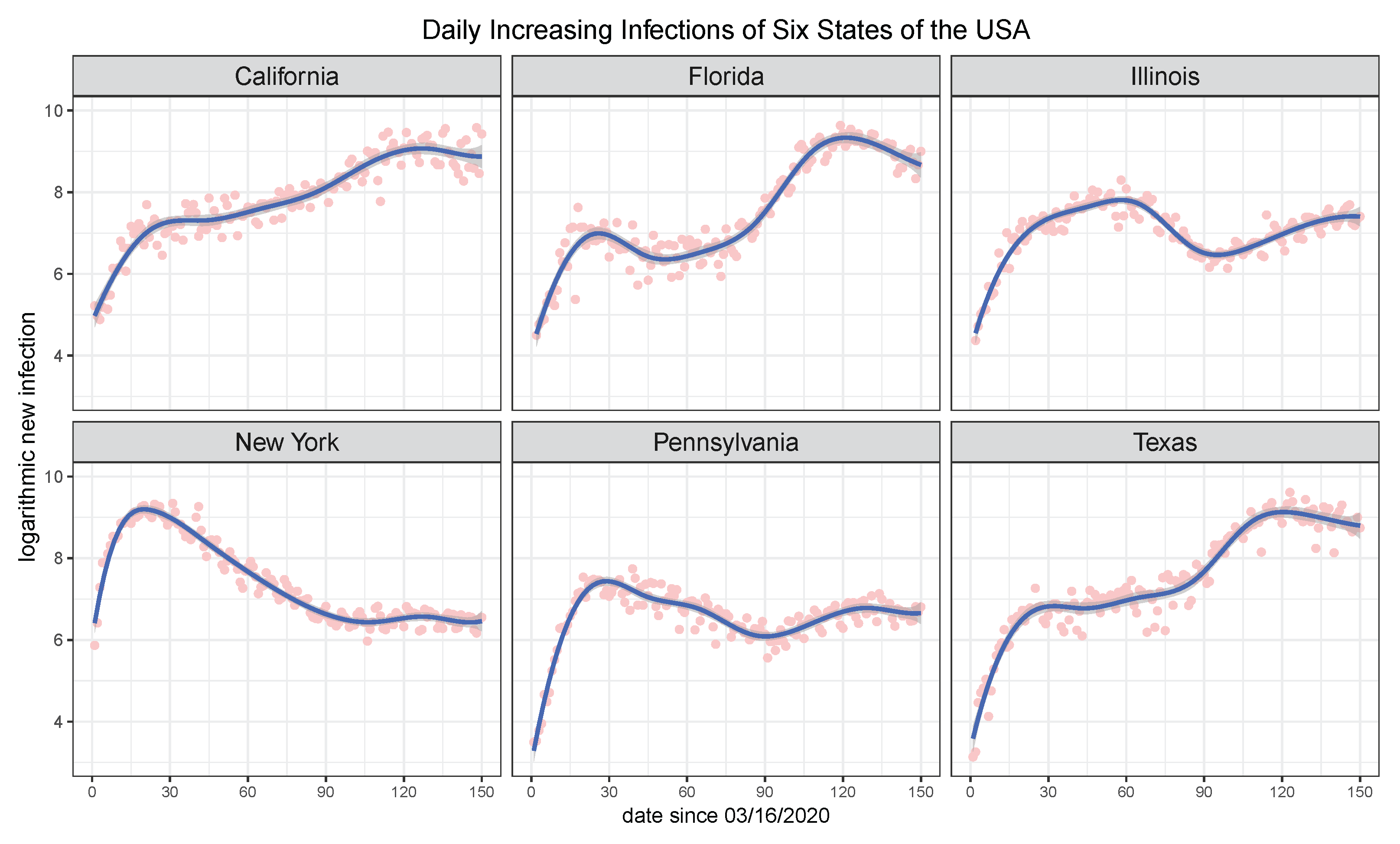
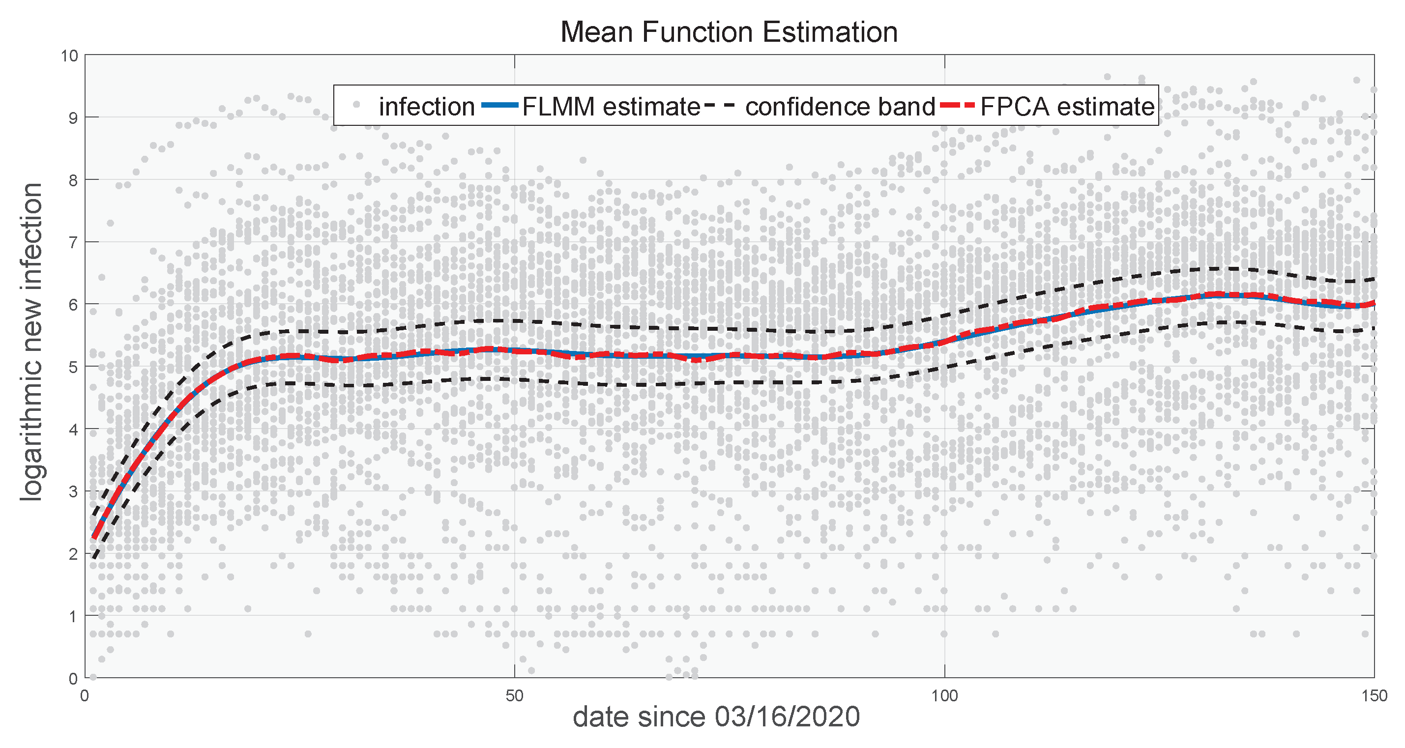
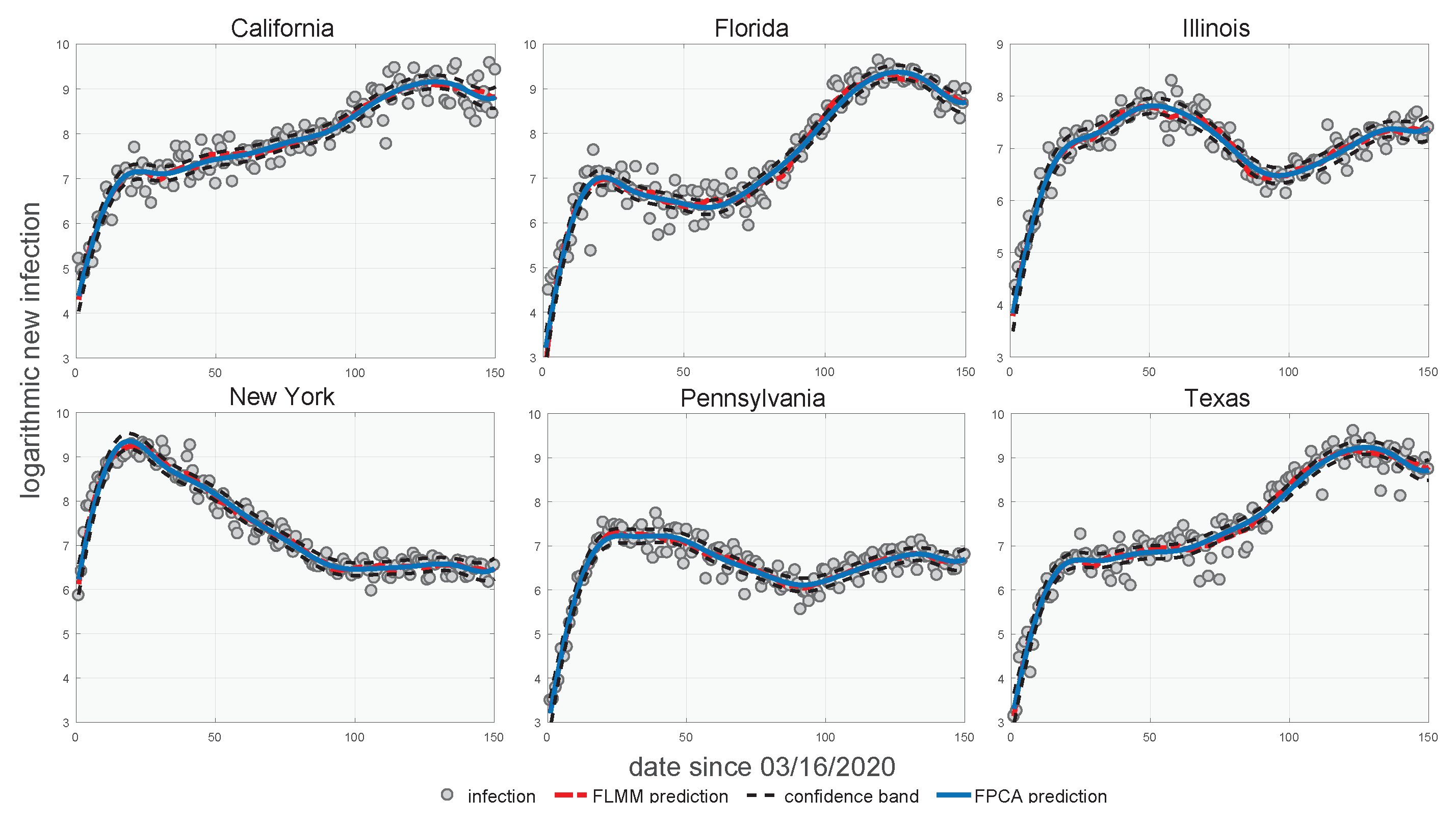
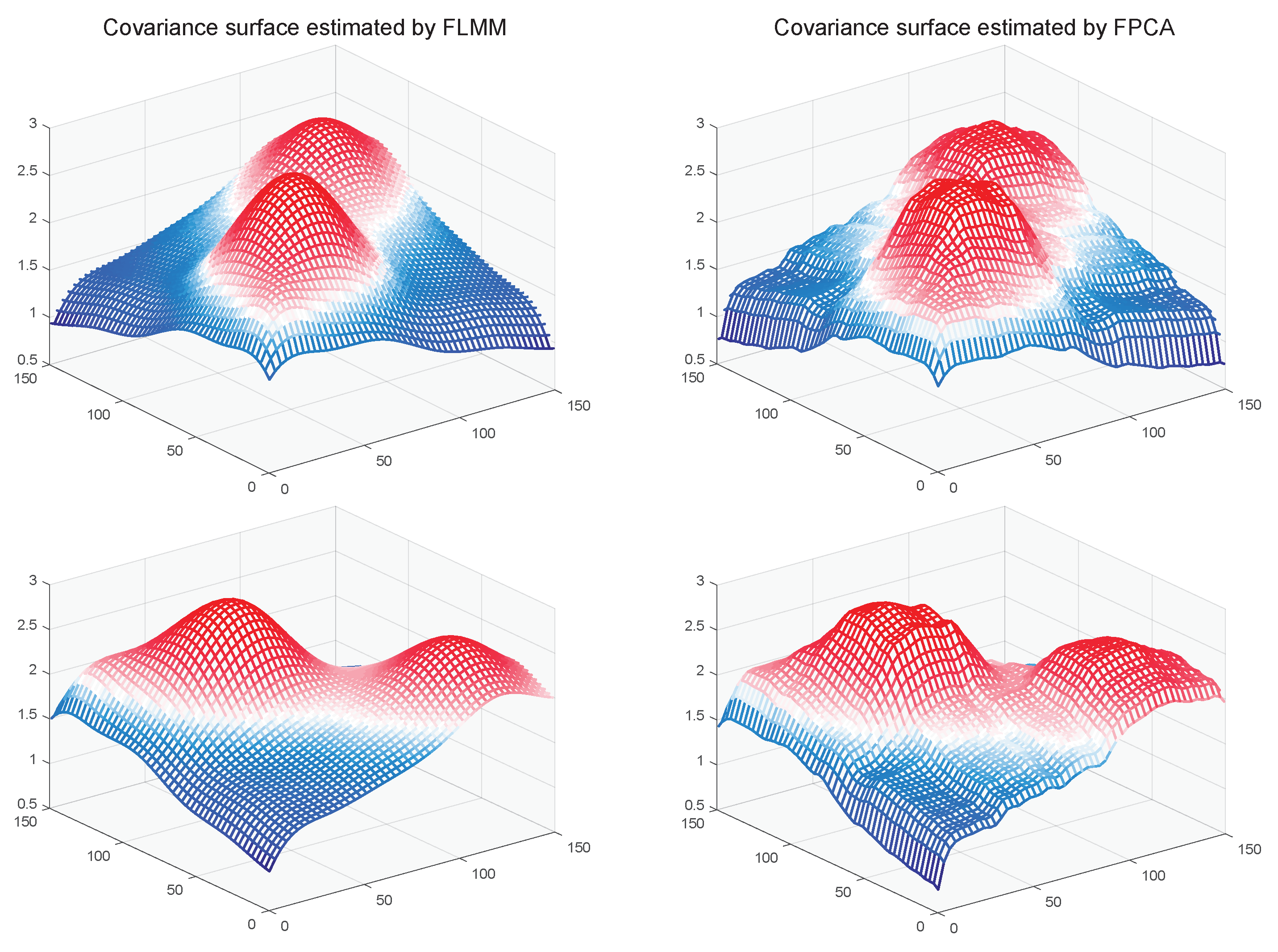
5. Real Data Analysis

We demonstrate the effectiveness of the proposed method via the analysis of the COVID-19 data in this section. This data is updated daily on the number of COVID-19 infectious cases and deaths in the 50 states and DC in the US by the Center for Systems Science and Engineering (CSSE) at Johns Hopkins University. It contains $N=51$ subjects and $T=152$ observations. The realization is the number of COVID-19 cases after the logarithm, which was recorded every day from 16 March 2020 to 14 August 2020. Partial observations are negative because of certain unknown reasons. For such an observation, we replace it with the average of the three observations around it. We employ 15 and 10 numbers of Bsplines bases to approximate the mean function and individual trajectories, respectively. It should be pointed out that we have not changed the default settings of the PACE package, and in our FLMM method, the number of employed bases p is the only tuning parameter to select. Therefore, the comparison between FPCA and FLMM is fair.

The results of this data analysis are shown in Figure 5, Figure 6 and Figure 7. Figure 5 displays the two estimated mean functions obtained by FPCA and our novel FLMM, respectively. The smaller panel within tries to draw attention to the stability of the two mean curves. The results further reveal the reason as to why FPCA performs worse than FLMM in terms of mean function estimation: it may overfit the mean function. Besides, due to the $N=51$ sample size, we chose six states with the top populations among all states to represent individual trajectories, and the consequence is shown in Figure 6. Likewise, FPCA tends to overfit the individual trajectories while FLMM with our new estimator can fit them accurately. In addition, Figure 7 demonstrated the estimated covariance surface yielded by the two approaches. Generally, the two covariance surfaces are similar; but the one generated by our FLMM is smoother than FPCA. In addition, in terms of computing time, our FLMM estimator only takes 0.088 seconds, while PACE takes 44.08 seconds. Such a substantial gap confirms that our FLMM estimator is much more efficient than FPCA in terms of computation. In conclusion, FPCA implemented by PACE is very likely to overfit the mean function estimation, individual trajectory prediction, and covariance function estimation.

6. Discussion

In this paper, we propose a novel estimator of large functional data using the FLMM technique. In comparison with the FPCA, this novel estimator is much more efficient because all parameters can be automatically estimated. In comparison with the traditional estimator of FLMM, i.e., the REML criterion, our novel estimator adopts the LAML criterion, which enjoys a significantly lower computational complexity when the number of observations T or the number of employed bases p is large. In the simulation, our novel estimator of FLMM outperforms or performs equally as FPCA in all five criteria. In real data analysis, it is able to provide more reliable estimates than PFCA in terms of avoiding overfitting. Note that we only compare the novel estimator with the FPCA implemented by the PACE package, because the computing time of the traditional estimator of FLMM with REML is extremely large, and it is very easy to encounter numerical problems such as a degenerate Hessian matrix.

Another contribution of this paper is the asymptotic theory of FLMM. As far as we are concerned, our work is the first one to point out the convergence rates of mean function estimate, individual trajectory prediction, variance estimate, and covariance surface estimate. Theorems 1 and 2 show that the mean function estimate and individual trajectory prediction can reach the minimax lower bounds if the numbers of employed bases are chosen optimally. In particular, we point out that the number of basis functions should be adaptively chosen when estimating the mean function and individual trajectory, providing a novel guide about how to perform FLMM in practice. However, Theorems 3 and 4 illustrate that the convergence rates of variance estimate and covariance surface estimate cannot reach the minimax lower bounds because of the estimation errors of mean function estimate and individual trajectory prediction. These two findings indicate that the variance components cannot be precisely estimated if the mean function estimate and individual trajectory prediction are not consistent.

It should be pointed out that the proposed estimator can be simply extended to analyze unbalanced longitudinal data or the so-called sparse functional data [11]. Indeed, the FLMM estimator of unbalanced longitudinal data resembles the combination of penalized quasi-likelihood (PQL) and REML/LAML; a similar estimating procedure can be found in Breslow and Clayton [33]. Since in unbalanced longitudinal data, the number of observations for each individual is usually small, the FLMM estimator will not suffer from the theoretical and computational difficulties caused by the “dimensional curse”. As mentioned before, Vonesh et al. [34] pointed out that the convergence rate of the mean parameter in GLMM is $O\left(T_{min}^{-1/2}\right)$. However, as far as we are concerned, the convergence rates of covariance matrix estimate and individual prediction are still unknown. As for FLMM, since the approximation bias of basis expansions is further involved, it is even unclear if the four estimates are consistent. Hence, it is worth future studying under what conditions the FLMM estimation is consistent for unbalanced longitudinal data or sparse functional data.

Discrete functional data analysis is an area that has received much less attention than continuous functional data analysis. However, discrete data are more common in longitudinal data analysis than continuous data, and hence the technical tools for analyzing discrete functional data are more urgently needed. Specifically, the model of discrete functional data is

$$\begin{array}{c}\hfill \mathrm{E}\left(Y_i\left(t_j\right)\right)=g^{-1}(X_i\left(t_j\right)+{\mathit{W}}_{ij}^{\top }\gamma ),\end{array}$$

(50)

where $Y_i\left(t_j\right)$ is a random variable following the exponential family distribution [45], $g(·)$ is the so-called link function, and ${\mathit{W}}_{ij}$ is certain vector of covariates. We conjecture that the convergence rates of mean function estimate, individual trajectory prediction, variance estimate, and covariance surface estimate in this new model are the same as the ones indicated by Theorems 1–4 if the sampling locations $\left\{t_j\right\}$ are balanced for all individuals. On the other hand, such a problem has been studied by Hall et al. [46] using the FPCA technique. It is also worth comparing the performances of FLMM and FPCA when dealing with such discrete functional data.

References

1. Ramsay, J.; Silverman, B. Functional Data Analysis; Springer: Berlin/Heidelberg, Germany, 2005. [Google Scholar]
2. Králík, M.; Klíma, O.; Ŏuta, M.; Malina, R.M.; Kozieł, S.; Polcerová, L.; Škultétyová, A.; Španěl, M.; Kukla, L.; Zemčík, P. Estimating Growth in Height from Limited Longitudinal Growth Data Using Full-Curves Training Dataset: A Comparison of Two Procedures of Curve Optimization—Functional Principal Component Analysis and SITAR. Children 2021, 8, 934. [Google Scholar] [CrossRef] [PubMed]
3. Ullah, S.; Finch, C. Applications of functional data analysis: A systematic review. BMC Med Res. Methodol. 2013, 13, 43. [Google Scholar] [CrossRef] [PubMed] [Green Version]
4. Cai, T.; Yuan, M. Nonparametric Covariance Function Estimation for Functional and Longitudinal Data; University of Pennsylvania and Georgia Inistitute of Technology: Philadelphia, PA, USA, 2010. [Google Scholar]
5. Diggle, P.; Diggle, P.; Heagerty, P.; Liang, K.; Zeger, S. Analysis of Longitudinal Data; Oxford University Press: Oxford, UK, 2002. [Google Scholar]
6. Wood, S.; Wood, M. Package ‘mgcv’. R Package Version 2015, 1, 729. [Google Scholar]
7. Patterson, H.; Thompson, R. Recovery of inter-block information when block sizes are unequal. Biometrika 1971, 58, 545–554. [Google Scholar] [CrossRef]
8. Laird, N.; Ware, J. Random-effects models for longitudinal data. Biometrics 1982, 1, 963–974. [Google Scholar] [CrossRef]
9. Hall, P.; Müller, H.; Wang, J. Properties of principal component methods for functional and longitudinal data analysis. Ann. Stat. 2006, 34, 1493–1517. [Google Scholar] [CrossRef] [Green Version]
10. Li, Y.; Hsing, T. Uniform convergence rates for nonparametric regression and principal component analysis in functional/longitudinal data. Ann. Stat. 2010, 38, 3321–3351. [Google Scholar] [CrossRef]
11. Yao, F.; Müller, H.; Wang, J. Functional data analysis for sparse longitudinal data. J. Am. Stat. Assoc. 2005, 100, 577–590. [Google Scholar] [CrossRef]
12. Paul, D.; Peng, J. Consistency of restricted maximum likelihood estimators of principal components. Ann. Stat. 2009, 37, 1229–1271. [Google Scholar] [CrossRef]
13. Peng, J.; Paul, D. A geometric approach to maximum likelihood estimation of the functional principal components from sparse longitudinal data. J. Comput. Graph. Stat. 2009, 18, 995–1015. [Google Scholar] [CrossRef] [Green Version]
14. Bunea, F.; Ivanescu, A.; Wegkamp, M. Adaptive inference for the mean of a Gaussian process in functional data. J. R. Stat. Soc. Ser. B (Stat. Methodol.) 2011, 73, 531–558. [Google Scholar] [CrossRef]
15. Rice, J.; Silverman, B. Estimating the mean and covariance structure nonparametrically when the data are curves. J. R. Stat. Soc. Ser. B (Stat. Methodol.) 1991, 53, 233–243. [Google Scholar] [CrossRef]
16. Yu, F.; Liu, L.; Yu, N.; Ji, L.; Qiu, D. A method of L1-norm principal component analysis for functional data. Symmetry 2020, 12, 182. [Google Scholar] [CrossRef] [Green Version]
17. James, G.; Hastie, T.; Sugar, C. Principal component models for sparse functional data. Biometrika 2000, 87, 587–602. [Google Scholar] [CrossRef] [Green Version]
18. James, G.; Sugar, C. Clustering for sparsely sampled functional data. J. Am. Stat. Assoc. 2003, 98, 397–408. [Google Scholar] [CrossRef]
19. Rice, J.; Wu, C. Nonparametric mixed effects models for unequally sampled noisy curves. Biometrics 2001, 57, 253–259. [Google Scholar] [CrossRef] [Green Version]
20. Shi, M.; Weiss, R.; Taylor, J. An analysis of paediatric CD4 counts for acquired immune deficiency syndrome using flexible random curves. J. R. Stat. Soc. Ser. C Appl. Stat. 1996, 45, 151–163. [Google Scholar] [CrossRef]
21. Antoniadis, A.; Sapatinas, T. Estimation and inference in functional mixed-effects models. Comput. Stat. Data Anal. 2007, 51, 4793–4813. [Google Scholar] [CrossRef]
22. Morris, J.; Carroll, R. Wavelet-based functional mixed models. J. R. Stat. Soc. Ser. B (Stat. Methodol.) 2006, 68, 179–199. [Google Scholar] [CrossRef] [Green Version]
23. Zhu, H.; Brown, P.; Morris, J. Robust, adaptive functional regression in functional mixed model framework. J. Am. Stat. Assoc. 2011, 106, 1167–1179. [Google Scholar] [CrossRef] [Green Version]
24. Qiu, P.; Zou, C.; Wang, Z. Nonparametric profile monitoring by mixed effects modeling. Technometrics 2010, 52, 265–277. [Google Scholar] [CrossRef]
25. Wu, H.; Zhang, J. Local polynomial mixed-effects models for longitudinal data. J. Am. Stat. Assoc. 2002, 97, 883–897. [Google Scholar] [CrossRef]
26. Wu, H.; Zhang, J. Nonparametric Regression Methods for Longitudinal Data Analysis: Mixed-Effects Modeling Approaches; John Wiley & Sons: Hoboken, NJ, USA, 2006. [Google Scholar]
27. Rice, J. Functional and longitudinal data analysis: Perspectives on smoothing. Stat. Sinica 2004, 1, 631–647. [Google Scholar]
28. Wang, J.; Chiou, J.; Müller, H. Functional data analysis. Annu. Rev. Stat. Appl. 2016, 3, 257–295. [Google Scholar] [CrossRef] [Green Version]
29. Cai, T.; Yuan, M. Optimal estimation of the mean function based on discretely sampled functional data: Phase transition. Ann. Stat. 2011, 39, 2330–2355. [Google Scholar] [CrossRef] [Green Version]
30. Fan, J.; Gijbels, I. Local Polynomial Modelling and Its Applications; Routledge: London, UK, 2018. [Google Scholar]
31. Eilers, P.; Marx, B. Flexible smoothing with B-splines and penalties. Stat. Sci. 1996, 11, 89–102. [Google Scholar] [CrossRef]
32. Acal, C.; Aguilera, A.; Escabias, M. New modeling approaches based on varimax rotation of functional principal components. Mathematics 2020, 8, 2085. [Google Scholar] [CrossRef]
33. Breslow, N.; Clayton, D. Approximate inference in generalized linear mixed models. J. Am. Stat. Assoc. 1993, 88, 9–25. [Google Scholar]
34. Vonesh, E.; Wang, H.; Nie, L.; Majumdar, D. Conditional second-order generalized estimating equations for generalized linear and nonlinear mixed-effects models. J. Am. Stat. Assoc. 2002, 97, 271–283. [Google Scholar] [CrossRef]
35. Breslow, N.; Lin, X. Bias correction in generalised linear mixed models with a single component of dispersion. Biometrika 1995, 82, 81–91. [Google Scholar] [CrossRef]
36. Lee, Y.; Nelder, J. Hierarchical generalized linear models. J. R. Stat. Soc. Ser. B (Stat. Methodol.) 1996, 58, 619–656. [Google Scholar] [CrossRef]
37. Lin, X.; Breslow, N. Bias correction in generalized linear mixed models with multiple components of dispersion. J. Am. Stat. Assoc. 1996, 91, 1007–1016. [Google Scholar] [CrossRef]
38. Ruppert, D.; Wand, M.; Carroll, R. Semiparametric Regression; Cambridge University Press: Cambridge, UK, 2003. [Google Scholar]
39. Wood, S.; Pya, N.; Säfken, B. Smoothing parameter and model selection for general smooth models. J. Am. Stat. Assoc. 2016, 111, 1548–1563. [Google Scholar] [CrossRef]
40. Vershynin, R. High-Dimensional Probability: An Introduction with Applications in Data Science; Cambridge University Press: Cambridge, UK, 2018. [Google Scholar]
41. Bickel, P.; Levina, E. Regularized estimation of large covariance matrices. Ann. Stat. 2008, 36, 199–227. [Google Scholar] [CrossRef]
42. Wainwright, M. High-Dimensional Statistics: A Non-asymptotic Viewpoint; Cambridge University Press: Cambridge, UK, 2019. [Google Scholar]
43. Tsybakov, A.B. Introduction to Nonparametric Estimation; Springer: Berlin/Heidelberg, Germany, 2009. [Google Scholar]
44. Wood, S. Fast stable restricted maximum likelihood and marginal likelihood estimation of semiparametric generalized linear models. J. R. Stat. Soc. Ser. B (Stat. Methodol.) 2011, 73, 3–36. [Google Scholar] [CrossRef] [Green Version]
45. Nelder, J.; Wedderburn, R. Generalized linear models. J. R. Stat. Soc. Ser. A (Gen.) 1972, 135, 370–384. [Google Scholar] [CrossRef]
46. Hall, P.; Müller, H.; Yao, F. Modelling sparse generalized longitudinal observations with latent Gaussian processes. J. R. Stat. Soc. Ser. B (Stat. Methodol.) 2008, 70, 703–723. [Google Scholar] [CrossRef]
47. Horn, R.; Johnson, C. Matrix Analysis; Cambridge University Press: Cambridge, UK, 2012. [Google Scholar]
48. Schwarz, G. Estimating the dimension of a model. Ann. Stat. 1978, 1, 461–464. [Google Scholar] [CrossRef]
Figure 1. Illustration of the COVID-19 data. The X-axis records the dates from 16 March 2020 to 14 August 2020 and the Y-axis shows the numbers of the logarithm of the daily infections.
Mathematics 10 04322 g001
Figure 2. The eigenfunctions, mean function, individual trajectory, and covariance function used in the simulation.
Mathematics 10 04322 g002
Figure 3. Estimation errors of mean function, individual trajectory, variance, covariance surface, and running time in the three methods.
Mathematics 10 04322 g003
Figure 4. Investigation of the covariance surface approximation.
Mathematics 10 04322 g004
Figure 5. Fitted mean functions of daily infection via FPCA and proposed FLMM.
Mathematics 10 04322 g005
Figure 6. Predictions of the trajectories of six states via FPCA and proposed FLMM.
Mathematics 10 04322 g006
Figure 7. Fitted covariance surfaces via FPCA and proposed FLMM.
Mathematics 10 04322 g007
Publisher’s Note: MDPI stays neutral with regard to jurisdictional claims in published maps and institutional affiliations.