
Interactive Impacts of Overconfidence and Competitive Preference on Closed-Loop Supply Chain Performance
Abstract
:1. Introduction
2. Literature Review
2.1. Closed-Loop Supply Chain Management
2.2. Bounded Rationality
2.3. Contributions
3. Model Setup
4. Analysis
4.1. Centralized Decision-Making Model (C)
4.2. Non-Leader Model ()
- A.
- The optimal wholesale price of the manufacturer increases in the competitive preference if, and only if, the retailer’s overconfidence level is of a high or low level, i.e.,
- B.
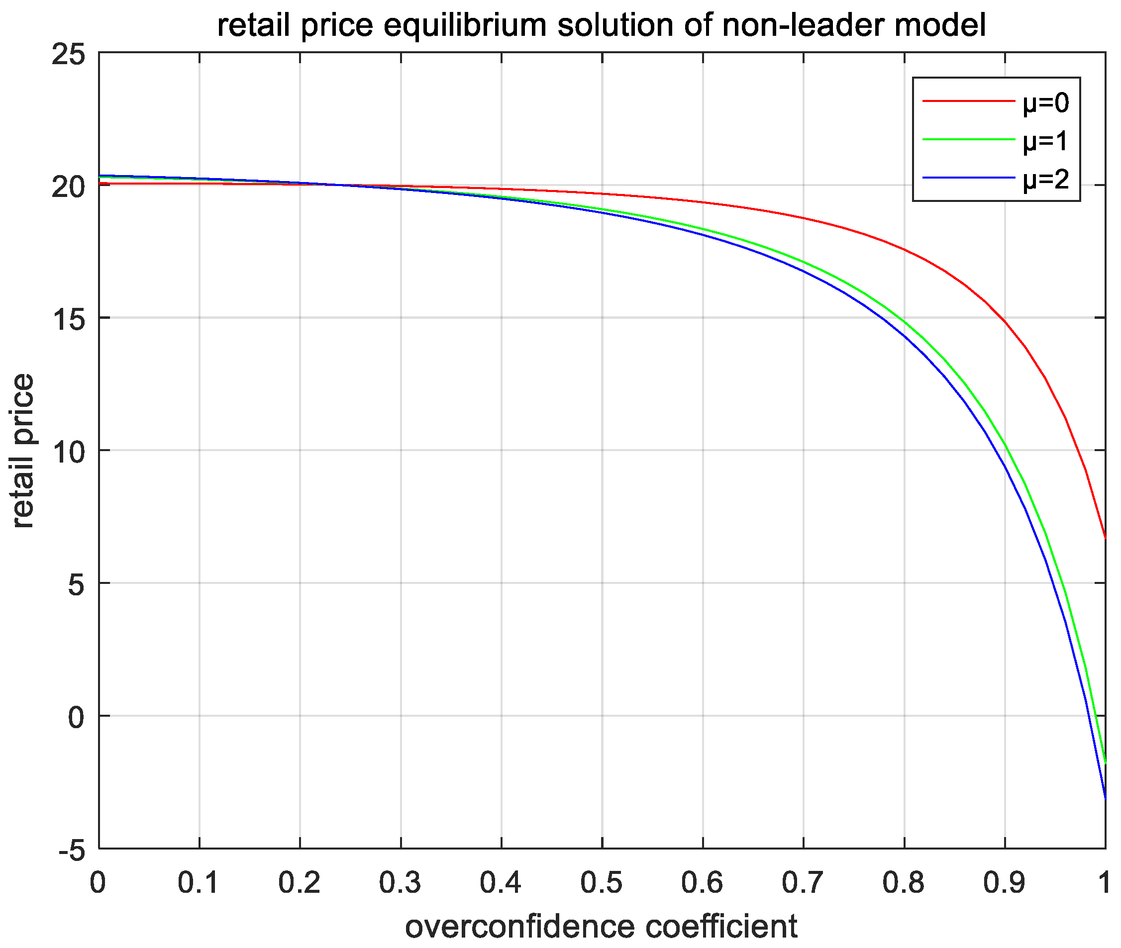
- The optimal selling price of the retailer increases in the competitive preference if, and only if, the retailer’s overconfidence level is of a high or low level and decreases otherwise, i.e.,
- C.
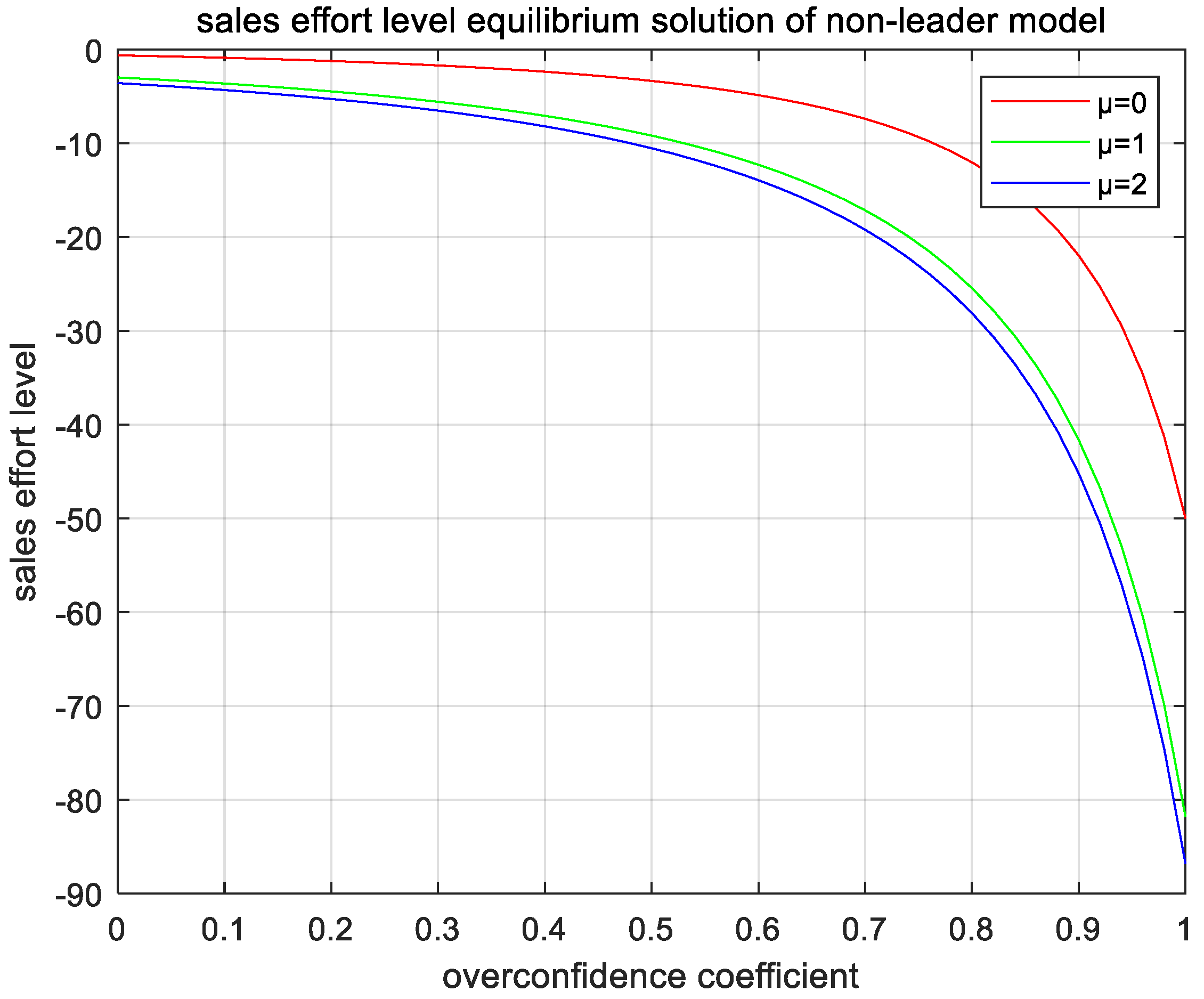
- The optimal sales effort of the retailer increases in the competitive preference with a high retailer’s overconfidence level and decreases otherwise, i.e.,where .
4.3. Manufacturer-Led Model ()
- A.
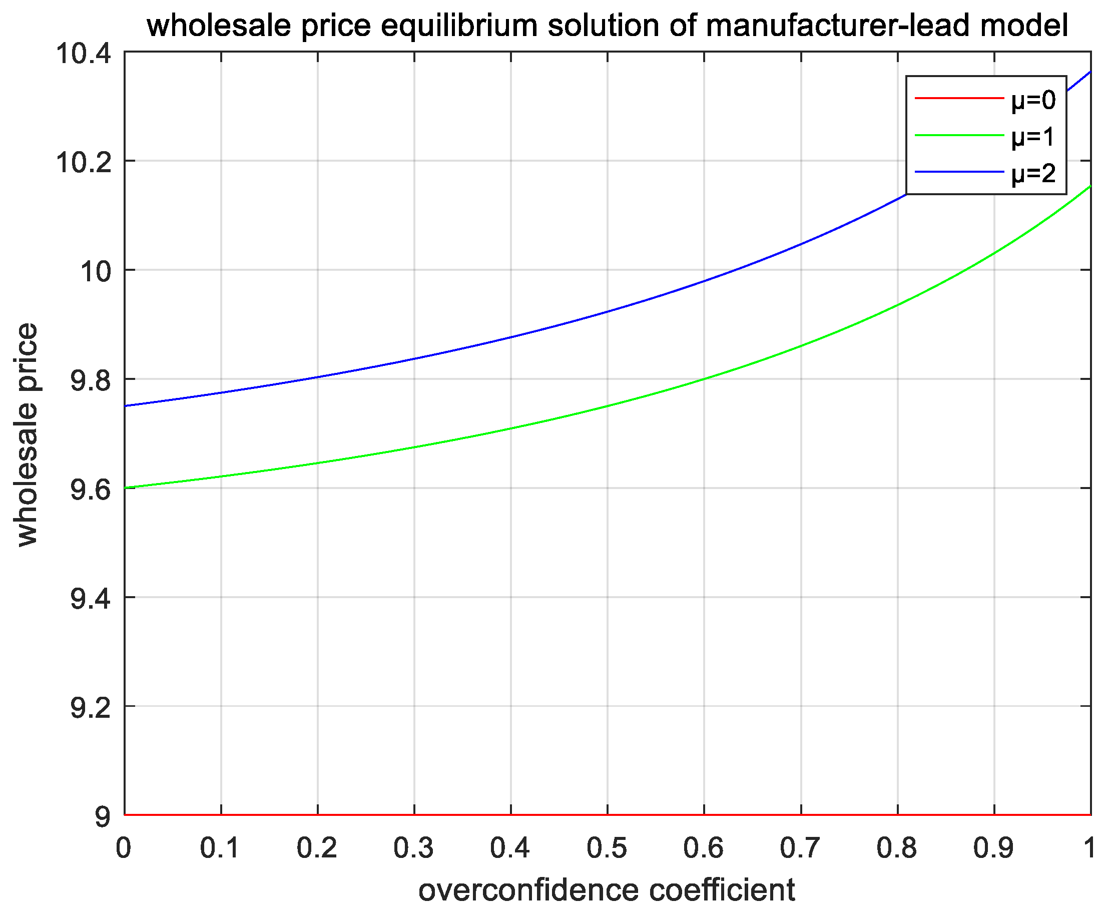
- The optimal wholesale price of the manufacturer increases in the competitive preference if, and only if, the retailer’s overconfidence level is of a high or low level, i.e.,
- B.
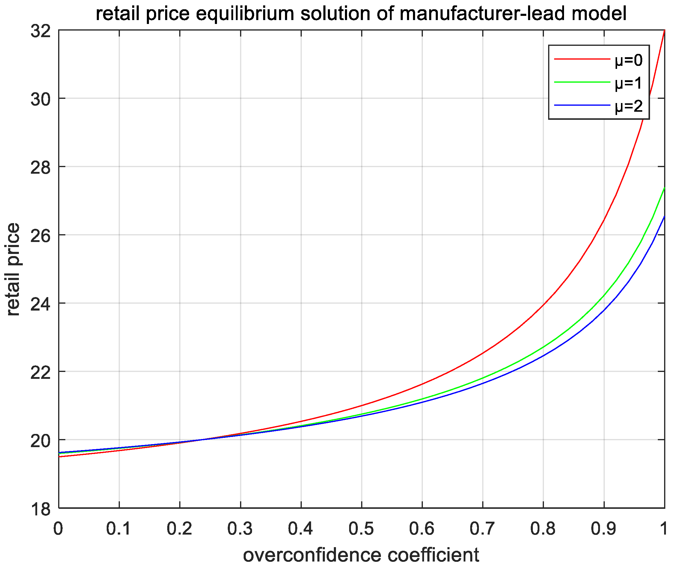
- The optimal selling price of the retailer increases in the competitive preference if, and only if, the retailer’s overconfidence level is of a high or low level and decreases otherwise, i.e.,
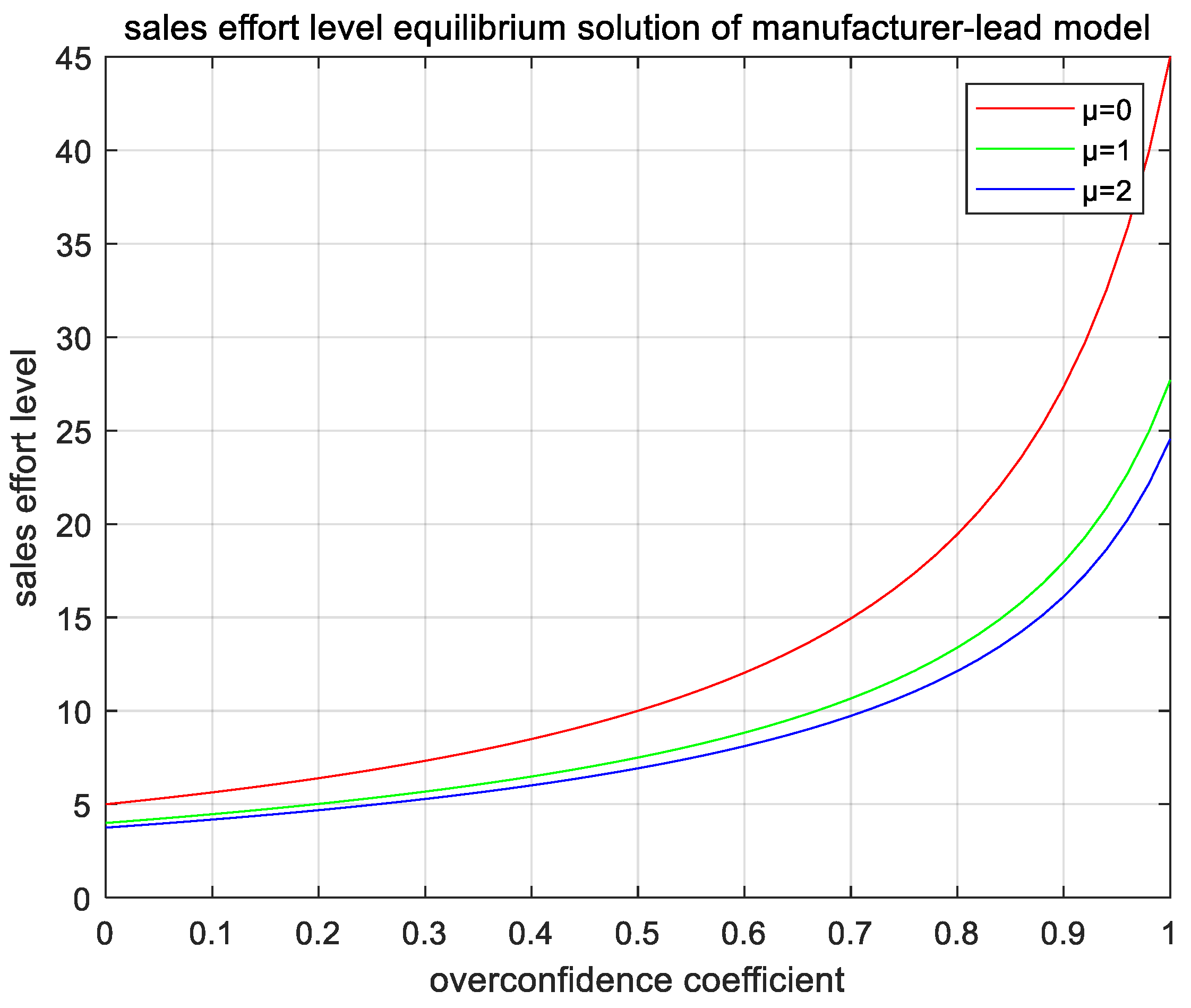
- C.
- The optimal sales effort of the retailer increases in the competitive preference with a high retailer overconfidence level and decreases otherwise, i.e.,where .
4.4. The Comparison between -Game and -Game
- A.
- For the retailer, the profits under the non-leader () model are larger than the profits under the manufacturer-led () model .
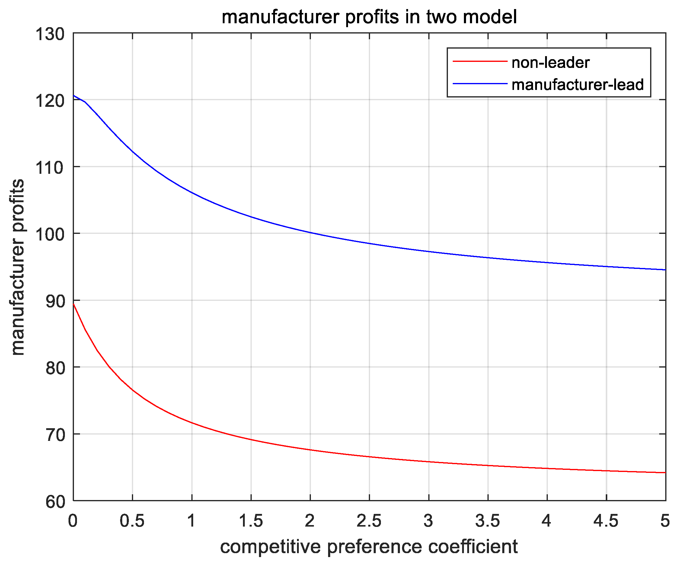
- B.
- For manufacturers, the profits under the manufacturer-led () model is larger than the profits under the non-leader () model .
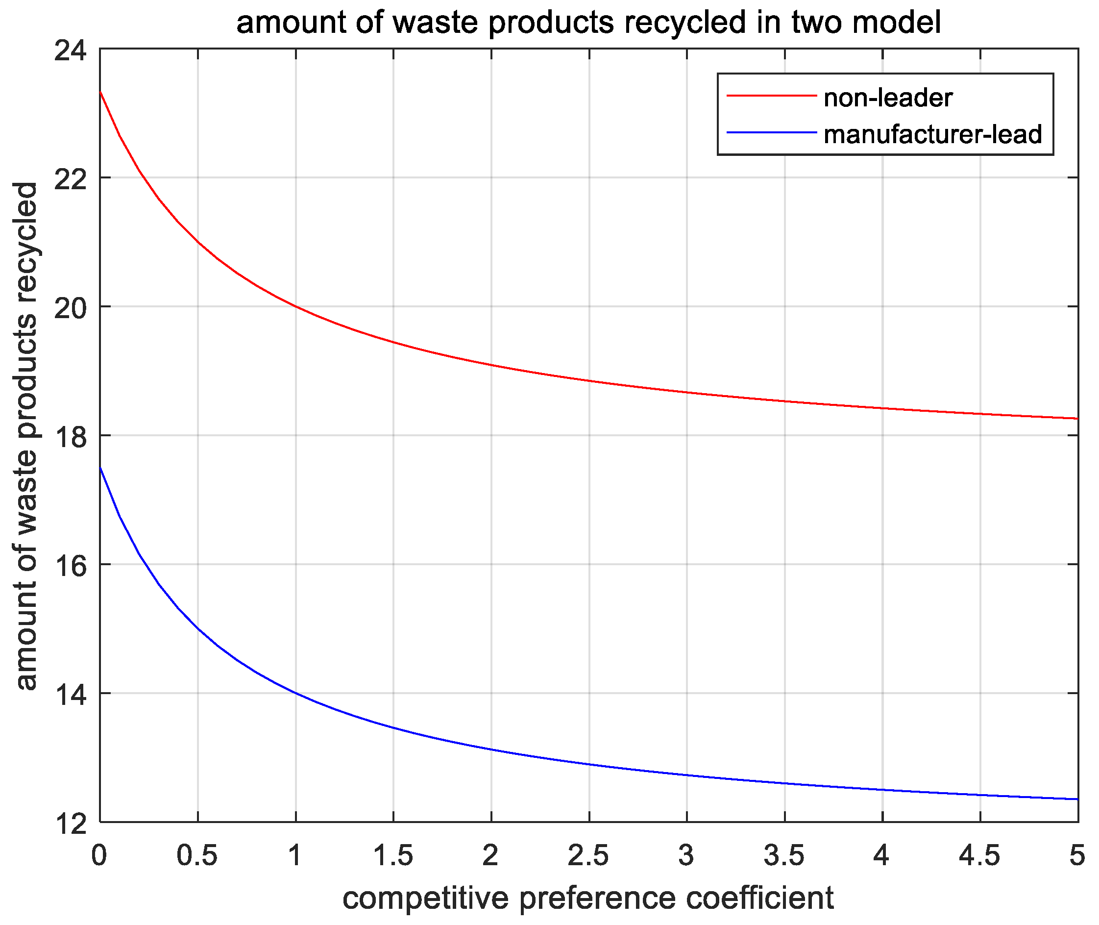
- C.
- The amount of waste products recycled under the manufacturer-led () model is smaller than that under the non-leader () model , and further smaller than that in the centralized decision model .
- D.
- The amount of used product recycled in the non-leader () model and the amount of used product recycled in the manufacturer-led () model are both inversely proportional to the competitive preference coefficient .
5. Conclusions
Author Contributions
Funding
Conflicts of Interest
Appendix A
Appendix B
References
- Masi, D.; Day, S.; Godsell, J. Supply Chain Configurations in the Circular Economy: A Systematic Literature Review. Sustainability 2017, 9, 1602. [Google Scholar] [CrossRef] [Green Version]
- Jabbour, C.J.C.; Fiorini, P.D.C.; Ndubisi, N.O.; Queiroz, M.M.; Piato, É.L. Digitally-enabled sustainable supply chains in the 21st century: A review and a research agenda. Sci. Total Environ. 2020, 725, 138177. [Google Scholar] [CrossRef] [PubMed]
- Simon, H.A. Theories of Bounded Rationality. In Decision & Organization; North-Holland Publishing Company: Amsterdam, The Netherlands, 2001; pp. 161–176. [Google Scholar]
- Li, P.; Ye, X. Research on Stackelberg Game and Countermeasures of Supply Chain under Retailer Cognitive Bias. Foreign Econ. Relat. Trade 2021, 5, 28–31. [Google Scholar]
- Zhang, Z.; Wang, P.; Wan, M.; Guo, J.; Luo, C. Interactive impacts of overconfidence and fairness concern on supply chain performance. Adv. Prod. Eng. Manag. 2020, 15, 277–294. [Google Scholar] [CrossRef]
- Russo, J.E.; Schoemaker, P.J.H. Managing overconfidence. Sloan Manag. Rev. 1992, 33, 7–17. [Google Scholar]
- Gary, C.; Matthew, R. Understanding Social Preferences with Simple Tests. Q. J. Econ. 2001, 117, 817–869. [Google Scholar]
- Gayialis, S.P.; Kechagias, E.P.; Papadopoulos, G.A.; Panayiotou, N.A. A Business Process Reference Model for the Development of a Wine Traceability System. Sustainability 2022, 14, 11687. [Google Scholar] [CrossRef]
- Zhang, F.-A.; Da, Q.; Sun, H. Analysis of Benefit for Closed-loop Supply Chain with Dominant Retailer. Soft Sci. 2011, 25, 45–48. [Google Scholar]
- Gao, J.; Han, H.; Hou, L. Decision-making in Closed-loop Supply Chain with Dominant Retailer Considering Products’ Green Degree and Sales Effort. Manag. Rev. 2015, 27, 10. [Google Scholar]
- Yao, F.M.; Xu, S.B.; Teng, C.X. Decision models for closed-loop supply chain with dominant retailer under dual recycle channels. Comput. Integr. Manuf. Syst. 2016, 22, 9. [Google Scholar]
- Yi, Y.-Y. Study on Closed-loop Supply Chain under Different Market Power. J. Syst. Manag. 2010, 4, 389–396. [Google Scholar]
- Wang, W.-B.; Da, Q.-L.; Nie, R. The Study on Pricing and Coordination of Closed-loop Supply Chain Considering Channel Power Structure. Chin. J. Manag. Sci. 2011, 19, 29–36. [Google Scholar] [CrossRef]
- Li, M.F.; Xue, J.M. Performance analysis of manufacturer collecting closed-loop supply chain under different channel power structures. Control. Decis. 2016, 31, 6. [Google Scholar]
- Gong, Y.-D. Optimal combination of dominant mode and recovery mode for supply chain stability. J. Syst. Eng. 2014, 29, 11. [Google Scholar]
- Telegraphi, A.H.; Bulgak, A.A. A Mathematical Model for the Sustainable Design of a Cellular Manufacturing System in the Tactical Planning of a Closed-Loop Supply Chain Featuring Alternative Routings and Outsourcing Option. J. Adv. Manuf. Syst. 2021, 20, 135–162. [Google Scholar] [CrossRef]
- Geyer, R.; van Wassenhove, L.N.; Atasu, A. The Economics of Remanufacturing under Limited Component Durability and Finite Product Life Cycles. Manag. Sci. 2007, 53, 88–100. [Google Scholar] [CrossRef] [Green Version]
- Zhu, C.; Zhang, J. Pricing and coordination of closed-loop supply chain considering retailer’s dual-channel and difference in recycled products quality. Comput. Integr. Manuf. Syst. 2021, 27, 3318–3328. [Google Scholar]
- Gao, W.; Chen, J. Research on the impact of closed-loop supply chain activity strategy on performance. Sci. Technol. Manag. Res. 2010, 30, 118–120, 123. [Google Scholar]
- Manavalan, E.; Jayakrishna, K. A review of Internet of Things (IoT) embedded sustainable supply chain for industry 4.0 requirements. Comput. Ind. Eng. 2019, 127, 925–953. [Google Scholar] [CrossRef]
- Kechagias, E.P.; Chatzistelios, G.; Papadopoulos, G.A.; Apostolou, P. Digital transformation of the maritime industry: A cybersecurity systemic approach. Int. J. Crit. Infrastruct. Prot. 2022, 37, 100526. [Google Scholar] [CrossRef]
- Ren, Y.; Croson, D.C.; Croson, R.T.A. The overconfident newsvendor. J. Oper. Res. Soc. 2017, 68, 496–506. [Google Scholar] [CrossRef]
- Kirshner, S.N.; Shao, L. The overconfident and optimistic price-setting newsvendor. Eur. J. Oper. Res. 2019, 277, 166–173. [Google Scholar] [CrossRef]
- Doyle, J.; Ojiako, U.; Marshall, A.; Dawson, I.; Brito, M. The anchoring heuristic and overconfidence bias among frontline employees in supply chain organizations. Prod. Plan. Control. 2021, 32, 549–566. [Google Scholar] [CrossRef]
- Liu, B.; Cai, G.G.; Tsay, A.A. Advertising in Asymmetric Competing Supply Chains. Prod. Oper. Manag. 2014, 23, 1845–1858. [Google Scholar] [CrossRef]
- Li, M. Overconfident distribution channels. Prod. Oper. Manag. 2019, 28, 1347–1365. [Google Scholar] [CrossRef]
- Xu, L.; Shi, X.; Du, P.; Govindan, K.; Zhang, Z. Optimization on pricing and overconfidence problem in a duopolistic supply chain. Comput. Oper. Res. 2019, 101, 162–172. [Google Scholar] [CrossRef]
- Cui, T.H.; Raju, J.S.; Zhang, Z.J. Fairness and Channel Coordination. Manag. Sci. 2007, 53, 1303–1314. [Google Scholar]
- Caliskan-Demirag, O.; Chen, Y.; Li, J. Channel coordination under fairness concerns and nonlinear demand. Eur. J. Oper. Res. 2010, 207, 1321–1326. [Google Scholar] [CrossRef]
- Nie, T.; Du, S. Dual-fairness Supply Chain with Quantity Discount Contracts. Eur. J. Oper. Res. 2017, 258, 491–500. [Google Scholar] [CrossRef]
- Wang, Y.; Yu, Z.; Shen, L. Study on the decision-making and coordination of an e-commerce supply chain with manufacturer fairness concerns. Int. J. Prod. Res. 2018, 57, 1–21. [Google Scholar] [CrossRef]
- Pan, K.; Cui, Z.; Lu, Q. Impact of Fairness Concern on Retailer-Dominated Supply Chain. Comput. Ind. Eng. 2020, 139, 106209. [Google Scholar] [CrossRef]
- Mukhopadhyay, S.K.; Yao, D.; Yue, X. Information sharing of value-adding retailer in a mixed channel hi-tech supply chain. J. Bus. Res. 2006, 61, 950–958. [Google Scholar] [CrossRef]
- Karray, S. Periodicity of pricing and marketing efforts in a distribution channel. Eur. J. Oper. Res. 2013, 228, 635–647. [Google Scholar] [CrossRef]
- Wu, Z.; Huang, M. Performance analysis of closed-loop supply chain with manufacturer’s competitive preferences. J. Syst. Eng. 2020, 35, 73–87. [Google Scholar]
- Chen, K.G.; Song, X.F.; Wang, X.Y.; Huang, M. Joint Pricing and Production Decisions with the Overconfident Sales Agent. J. Syst. Manag. 2016, 25, 468–476. [Google Scholar]


| Notation | Definition |
|---|---|
| A | Potential demand size in the market |
| Price elasticity coefficient | |
| p | Retailing price |
| w | Wholesaling price |
| e | Retailers’ sales effort level |
| Output coefficient of the retailer’s sales effort | |
| c(e) | Cost of sales effort for retailers |
| Cost of sales effort factor | |
| The manufacturer’s/retailer’s marginal cost | |
| The marginal production cost of the manufacturer | |
| Retailer’s overconfidence parameter | |
| Demand in the absence of overconfidence | |
| D | Demand in the presence of overconfidence |
| l | Basic recycling volume in the market |
| h | Price elasticity of recycling of waste and scrap products |
| The manufacturer’s/retailer’s recycling price | |
| G | Total number of waste products recycled in the market |
| Production cost saving from recycling | |
| Manufacturer’s competitive preference coefficient | |
| Indicates profit of manufacture/retailer/system | |
| Indicates utility of manufacturer |
Publisher’s Note: MDPI stays neutral with regard to jurisdictional claims in published maps and institutional affiliations. |
© 2022 by the authors. Licensee MDPI, Basel, Switzerland. This article is an open access article distributed under the terms and conditions of the Creative Commons Attribution (CC BY) license (https://creativecommons.org/licenses/by/4.0/).
Share and Cite
Xu, H.; Gao, K.; Chi, Y.; Chen, Y.; Peng, R. Interactive Impacts of Overconfidence and Competitive Preference on Closed-Loop Supply Chain Performance. Mathematics 2022, 10, 4334. https://doi.org/10.3390/math10224334
Xu H, Gao K, Chi Y, Chen Y, Peng R. Interactive Impacts of Overconfidence and Competitive Preference on Closed-Loop Supply Chain Performance. Mathematics. 2022; 10(22):4334. https://doi.org/10.3390/math10224334
Chicago/Turabian StyleXu, Hao, Kaiye Gao, Yuanying Chi, Yahui Chen, and Rui Peng. 2022. "Interactive Impacts of Overconfidence and Competitive Preference on Closed-Loop Supply Chain Performance" Mathematics 10, no. 22: 4334. https://doi.org/10.3390/math10224334