Sustainable Urban Conveyance Selection through MCGDM Using a New Ranking on Generalized Interval Type-2 Trapezoidal Fuzzy Number

Abstract

This article proposes a modified ranking technique for generalized interval type-2 trapezoidal fuzzy numbers. For demonstrating uncertainty and managing imprecision in decision-making information, interval type-2 fuzzy sets are beneficial. The proposed ranking methodology resolves the difficulty of multi-criteria group decision-making on sustainable urban conveyance. Additionally, the proposed ranking approach considers all crucial aspects of transportation sustainability, including the effectiveness of durable transportation systems from economic, social, and ecological perspectives in multi-criteria group decision-making scenarios. The new ranking methodology yields superior outcomes for choosing sustainable urban transportation options. In the numerical part, studies compared the proposed ranking approach to other methods currently used for various MCDM techniques.

1. Introduction

The twentieth century was forced to rely primarily on non-renewable fossil resources. The impacts of fossil fuels have been extensively studied in the twenty-first century, and it has been determined that renewable energy should be used instead. When global awareness is so concerned with, and concentrating on, sustainability, providing transport solutions that work for everyone can be challenging. There are various factors to consider, such as price, environmental impact, and safety. This article addresses current and future solutions for durable transportation.

The term “sustainable transportation (ST)” refers to any mode of travel considered “green”, having minimal negative effect on the surrounding natural environment. Durable transportation also involves striking a balance between our present and future requirements. Walking, cycling, public transit, carpooling, car sharing, and driving environmentally friendly automobiles are all forms of durable mobility. Moreover, ST includes low and zero-emission, energy-efficient, inexpensive modes of transport, like electric and alternative-fuel vehicles. Future economic, social, and environmental factors will all play a role in a country’s ST performance and in the development of sustainable transportation technologies for durable transportation [1,2]. Local communities typically provide some form of public transportation as an alternative mode of conveyance that allows more people to travel together along predetermined paths. Buses, trains, and trams are all common forms of public vehicles that are commonly used. Most public transit between cities is provided by high-speed trains, aircraft, and coaches. As a result, public transportation can help to reduce traffic congestion, reduce exhaust emissions emitted by idle automobiles, and alleviate some of the stress associated with regular journeys in congested locations. However, there is an imprecise and uncertain situation regarding people’s choice of sustainable urban transportation. We can use decision-making techniques to overcome these ambiguous and uncertain situations.

The circumstances are ambiguous and imprecise in various problem definitions, making it difficult to solve the problems. Due to the uncertain and imprecise situation in ST systems, choosing the best alternative is challenging. Fuzziness helps us to deal with ambiguous and unclear data. Choosing sustainable urban transportation is usually inaccurate and unreliable, with uncertain and vague data. Fuzzy numbers allow us to deal with uncertain and ambiguous situations by solving fuzzy decision-making problems using various multi-criteria techniques. The phrase “fuzzy decision-making” refers to a group of single- or multi-criteria methods used to determine the best solution in situations where the data is imprecise, incomplete, or hazy.

In the context of this discussion, the term “multi-criteria techniques” refers to “multi-criteria decision-making” (MCDM) or “multi-criteria decision analysis” (MCDA). The MCDM concept is “a method used to combine the performance of several alternatives based on a wide range of competing alternatives for qualitative and/or quantitative criteria, which ultimately results in a solution that requires consensus”. The study of MCDM is a popular and comprehensive application in different fields and a variety of environments [3,4,5,6,7,8,9,10,11,12,13,14,15,16,17,18,19,20,21,22,23,24,25,26,27,28,29,30,31]. When the criteria are more complicated, or cannot be appraised by a single decision-maker, we need the opinions of two or more decision-makers to reach a conclusion. This type of decision-making is called multi-criteria group decision-making (MCGDM). In the consensus decision-making process, the group agrees on the problem. It freely communicates ideas and views on potential solutions through consensus decision-making.

2. Literature Review

Several authors offered and contributed their ideas for an ST system in a fuzzy environment, utilizing different decision-making strategies, which is briefly illustrated in Table 1 and Figure 1. The use of MCDM techniques to select sustainable urban transportation alternatives using generalized interval type-2 trapezoidal fuzzy numbers (GIT2TrFN) is presented in this article. In the literature review, many authors contributed ideas and methodologies related to ST using different fuzziness techniques. Karjalainen and Juhola [3] proposed a list of public transportation sustainability indicators. Avineri et al. [4] proposed a transportation project selection process using the fuzzy sets theory. Rajak et al. [5] evaluated ST system performance. Hansson et al. [6] analyzed the quality attributes of regional public transport. Stefaniec et al. [7] introduced an initial approach to measuring the social sustainability of regional transportation. Liang et al. [8] suggested vehicles powered by alternative fuels for ST. Gupta [9] evaluated several policy alternatives to decrease CO₂ emissions from road transport in India using the fuzzy MCDM technique. Kennedy [10] investigated the sustainability of the Toronto region’s public and private conveyance systems. The MCDM approach for the selection of environmentally friendly transportation was examined by Dragan et al. The change process in urban transport was studied by Wang et al. [12] using the transition theory of socio-technical systems to identify the best sustainable transition-promoting strategies. Figure 2 depicts a variety of real-life application problems in sustainable conveyance solved by various authors using MCDM and MCGDM techniques for the period 2000–2022.

The concept of sustainability is currently advancing and emphasizes the importance of both long-term strategic vision and immediate action planning and implementation in all fields of study ([32,33,34,35,36,37,38,39,40,41]). Environmental issues had not been pointed out as an effect of transportation in the early decades of the 2000s. At a later stage, researchers focused on sustainable transportation (refer to Table 1) to ensure environmental suitability for society. Fuzziness was incorporated due to the unavailability of data to make precise decisions on convenient conveyance for sustainable development. Figure 3 depicts the number of articles published on ST using fuzzy environments between 2000 and 2022.

Table 1. Literature survey on decision-making approaches to sustainable transport under a fuzzy environment.

Authors	Year	Methodology/Fuzziness	Type of DM	Applicability
Yedla & Shrestha [14]	2003	AHP	MCDM	The ST system in Delhi
Awasthi et al. [15]	2011	Fuzzy TOPSIS	MCDM	Selection of ST systems in cities
Rossi et al. [16]	2014	Fuzzy-based evaluation method	MCDM	Sustainability evaluation of transportation policies
Wei et al. [17]	2016	MCDA	MCDM	Selecting ST projects
Deveci et al. [19]	2018	TOPSIS & WASPAS	MCDM	Selection of a car-sharing station
Shankar et al. [20]	2018	Intuitionistic Fuzzy set	-	Sustainable freight transportation systems
Tan et al. [21]	2018	Adaptive neuro-fuzzy inference	MCDM	Urban sustainability transportation assessment
Buyukozkan et al. [22]	2018	Intuitionistic fuzzy	MCGDM	Selection of sustainable urban transportation
Moslem et al. [23]	2019	Fuzzy AHP & Interval AHP	MCDM	Stakeholder consensus for ST development decision
Liang et al. [8]	2019	Fuzzy AHP	MCGDM	Prioritization of alternative-fuel-based vehicles
Kumar et al. [24]	2020	VIKOR	MCDM	Evaluation of public road transportation Systems
Svadlenka et al. [25]	2020	Picture fuzzy DM	MCDM	Selection of sustainable LMD
Hamurcu & Eren [28]	2020	Fuzzy-AHP & TOPSIS	MCDM	Green transportation
Lv et al. [12]	2020	Fuzzy logic & TOPSIS	MCDM	Sustainability urban transportationevaluation
Ghorabaee [30]	2021	Fuzzy BWM & MABAC	MCDM	Sustainable public transportation evaluation
Pamucar et al. [11]	2021	FUCOM & neutrosophic fuzzy	MCDM	Fuel vehicles for sustainable road transportation
Ziemba [32]	2021	TOPSIS & SAW	Fuzzy MCDA	Selection of Electric Vehicles
Ania et al. [33]	2021	ELECTRE TRI	MCDM	Sustainable urban public transport systems
Broniewicz & Ogrodnik [34]	2021	Fuzzy AHP TOPSIS PROMETHEE	MCDA	Comparative Evaluation of MCDA for ST
Gutierrez [35]	2021	AHP	MCDA	Sustainable urban public transport systems
Lazaroiu & Roscia [37]	2022	Fuzzy logic	MCDM	Priority control of electric vehicle charging
Tirkolaee & Ayd1n [39]	2022	Fuzzy bi-level	MCDM	Decision support system for perishable products
Demir et al. [40]	2022	Fuzzy-fucom fuzzy-cocoso	MCDM	Toward sustainable urban mobility
Goyal et al. [41]	2021	Fuzzy-AHP fuzzy-TOPSIS	MCDM	Sustainable production and consumption
Xu et al. [42]	2022	Fuzzy comprehensive evaluation	MCDA	Smart city sustainable development
Prez et al. [43]	2015	Review more than 30 years	MCDM	Urban passenger transport systems
Pamucar et al. [44]	2021	BWM TODIM	MCDM	Zero-carbon city policies
Bakioglu & Atahan [45]	2021	Fuzzy-AHP TOPSIS VIKOR	MCDM	Prioritize the risks in self-driving vehicles
Zarbakhshnia et al. [46]	2018	Fuzzy SWARA fuzzy COPRAS	MCDM	Sustainable third-party reverse logistics provider
Yang et al. [47]	2022	LPHFS MULTIMOORA	MCDM	Selection of electric vehicle power battery recycling
Hajduk [48]	2022	TOPSIS	-	Linear ordering of urban transportation
This paper	2022	Fuzzy TOPSIS	MCGDM	Sustainable urban conveyance selection

Table 1. Literature survey on decision-making approaches to sustainable transport under a fuzzy environment.

Authors	Year	Methodology/Fuzziness	Type of DM	Applicability
Yedla & Shrestha [14]	2003	AHP	MCDM	The ST system in Delhi
Awasthi et al. [15]	2011	Fuzzy TOPSIS	MCDM	Selection of ST systems in cities
Rossi et al. [16]	2014	Fuzzy-based evaluation method	MCDM	Sustainability evaluation of transportation policies
Wei et al. [17]	2016	MCDA	MCDM	Selecting ST projects
Deveci et al. [19]	2018	TOPSIS & WASPAS	MCDM	Selection of a car-sharing station
Shankar et al. [20]	2018	Intuitionistic Fuzzy set	-	Sustainable freight transportation systems
Tan et al. [21]	2018	Adaptive neuro-fuzzy inference	MCDM	Urban sustainability transportation assessment
Buyukozkan et al. [22]	2018	Intuitionistic fuzzy	MCGDM	Selection of sustainable urban transportation
Moslem et al. [23]	2019	Fuzzy AHP & Interval AHP	MCDM	Stakeholder consensus for ST development decision
Liang et al. [8]	2019	Fuzzy AHP	MCGDM	Prioritization of alternative-fuel-based vehicles
Kumar et al. [24]	2020	VIKOR	MCDM	Evaluation of public road transportation Systems
Svadlenka et al. [25]	2020	Picture fuzzy DM	MCDM	Selection of sustainable LMD
Hamurcu & Eren [28]	2020	Fuzzy-AHP & TOPSIS	MCDM	Green transportation
Lv et al. [12]	2020	Fuzzy logic & TOPSIS	MCDM	Sustainability urban transportationevaluation
Ghorabaee [30]	2021	Fuzzy BWM & MABAC	MCDM	Sustainable public transportation evaluation
Pamucar et al. [11]	2021	FUCOM & neutrosophic fuzzy	MCDM	Fuel vehicles for sustainable road transportation
Ziemba [32]	2021	TOPSIS & SAW	Fuzzy MCDA	Selection of Electric Vehicles
Ania et al. [33]	2021	ELECTRE TRI	MCDM	Sustainable urban public transport systems
Broniewicz & Ogrodnik [34]	2021	Fuzzy AHP TOPSIS PROMETHEE	MCDA	Comparative Evaluation of MCDA for ST
Gutierrez [35]	2021	AHP	MCDA	Sustainable urban public transport systems
Lazaroiu & Roscia [37]	2022	Fuzzy logic	MCDM	Priority control of electric vehicle charging
Tirkolaee & Ayd1n [39]	2022	Fuzzy bi-level	MCDM	Decision support system for perishable products
Demir et al. [40]	2022	Fuzzy-fucom fuzzy-cocoso	MCDM	Toward sustainable urban mobility
Goyal et al. [41]	2021	Fuzzy-AHP fuzzy-TOPSIS	MCDM	Sustainable production and consumption
Xu et al. [42]	2022	Fuzzy comprehensive evaluation	MCDA	Smart city sustainable development
Prez et al. [43]	2015	Review more than 30 years	MCDM	Urban passenger transport systems
Pamucar et al. [44]	2021	BWM TODIM	MCDM	Zero-carbon city policies
Bakioglu & Atahan [45]	2021	Fuzzy-AHP TOPSIS VIKOR	MCDM	Prioritize the risks in self-driving vehicles
Zarbakhshnia et al. [46]	2018	Fuzzy SWARA fuzzy COPRAS	MCDM	Sustainable third-party reverse logistics provider
Yang et al. [47]	2022	LPHFS MULTIMOORA	MCDM	Selection of electric vehicle power battery recycling
Hajduk [48]	2022	TOPSIS	-	Linear ordering of urban transportation
This paper	2022	Fuzzy TOPSIS	MCGDM	Sustainable urban conveyance selection

According to the above literature review, no authors proposed a generalized method for dealing with ambiguities and imprecise data in decision-making problems. In this paper, we propose a new ranking of the GIT2TrN, which is an extension of the type-1 interval trapezoidal fuzzy number. More comprehensive coverage of the uncertainty zone is the option that favors the people making the decisions. Therefore, we need to consider the GIT2TrNs, rather than the type-1 interval trapezoidal fuzzy number. We used the fuzzy TOPSIS technique to validate the proposed new ranking method and considered the MCDM on sustainable urban transportation systems. Numerical examples on decision-making under fuzziness indicated the validity of the proposed approach.

This paper is structured as follows. In the first section, a brief introduction to ST is provided. In the second section, a short literature review provides a selection of sustainable transport via various fuzzy MCDM approaches. In the third section, the methodology of the proposed method and developments of fuzziness on GIT2TrFN are addressed. In the fourth section, proposed ranking methods are provided. In the fifth section, a numerical example of fuzzy MCGDM on ST is described. A sensitivity assessment demonstrates the numerical example problem. In the sixth section, the conclusion of the proposed ranking approach is presented.

3. Methodology

This article develops fuzzy MCGDM techniques, which are crucial topics applied in operations research. Due to its simplicity of use and high productivity, TOPSIS is one of the MCDM methodologies most frequently used. In this paper, the decision maker constructs the decision matrix with linguistic terms, such as GIT2TrFNs, and then applies the proposed ranking approach and fuzzy TOPSIS method. The defuzzification of GIT2TrFNs is used for computing the decision matrix. This approach makes the methodology as realistic as possible while making its application as simple as possible.

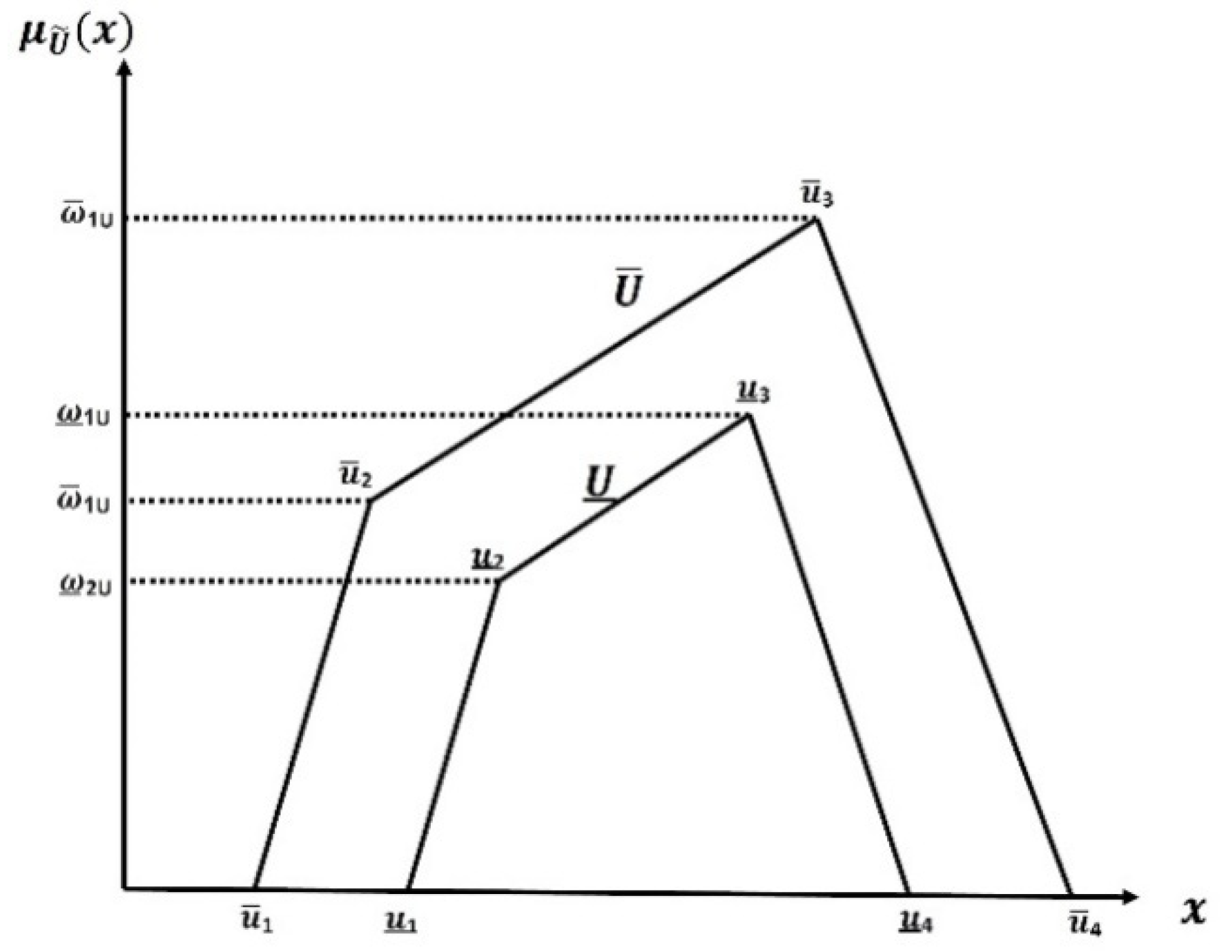
3.1. Developments of Fuzziness on GIT2TrFN

In this subsection, we discuss the development of interval type-2 fuzzy.

Definition 1.

A GIT2TrFN $\tilde{U}$ is defined on the interval $\left[{\overline{u}}_1,{\overline{u}}_4\right]$ with its LMF taking values equal to ${\underset{\_}{\omega }}_1$, ${\underset{\_}{\omega }}_2\in \left[0,1\right]$ in the points ${\underset{\_}{u}}_2,{\underset{\_}{u}}_3,$ respectively, and its UMF-taking values equal ${\overline{\omega }}_1$, ${\overline{\omega }}_2\in \left[0,1\right]$ in the points ${\overline{u}}_2,{\overline{u}}_3$, respectively. Therefore, the GIT2TrFN, $\tilde{U}$ notated as $\tilde{U}=\left(\left({\underset{\_}{u}}_1,{\underset{\_}{u}}_2,{\underset{\_}{u}}_3,{\underset{\_}{u}}_4;{\underset{\_}{\omega }}_1,{\underset{\_}{\omega }}_2\right),\left({\overline{u}}_1,{\overline{u}}_2,{\overline{u}}_3,{\overline{u}}_4;{\overline{\omega }}_1,{\overline{\omega }}_2\right)\right)$. Its membership functions (Figure 4) are:

$${\mu }_{\underset{\_}{U}}\left(x\right)=\{\begin{array}{ll}{\mu }_{{\underset{\_}{U}}_1\left(x\right)}={\underset{\_}{\omega }}_1\frac{x-{\underset{\_}{u}}_1}{{\underset{\_}{u}}_2-{\underset{\_}{u}}_1}\hfill & \mathrm{for} {\underset{\_}{u}}_1\le x\le {\underset{\_}{u}}_2,\hfill \\ {\mu }_{{\underset{\_}{U}}_2\left(x\right)}=\left({\underset{\_}{\omega }}_2-{\underset{\_}{\omega }}_1\right)\frac{x-{\underset{\_}{u}}_2}{{\underset{\_}{u}}_3-{\underset{\_}{u}}_2}+{\underset{\_}{\omega }}_1\hfill & \mathrm{for} {\underset{\_}{u}}_2\le x\le {\underset{\_}{u}}_3,\hfill \\ {\mu }_{{\underset{\_}{U}}_3\left(x\right)}={\underset{\_}{\omega }}_2\frac{{\underset{\_}{u}}_4-x}{{\underset{\_}{u}}_4-{\underset{\_}{u}}_3}\hfill & \mathrm{for} {\underset{\_}{u}}_3\le x\le {\underset{\_}{u}}_4,\hfill \\ {\mu }_{{\underset{\_}{U}}_4\left(x\right)}=0\hfill & \mathrm{for} x\le {\underset{\_}{u}}_1,x\ge {\underset{\_}{u}}_4.\hfill \end{array}$$

$$\mathrm{and} {\mu }_{\overline{U}}\left(x\right)=\{\begin{array}{ll}{\mu }_{{\overline{U}}_1\left(x\right)}={\overline{\omega }}_1\frac{x-{\overline{u}}_1}{{\overline{u}}_2-{\overline{u}}_1}\hfill & \mathrm{for} {\overline{u}}_1\le x\le {\overline{u}}_2,\hfill \\ {\mu }_{{\overline{U}}_2\left(x\right)}=\left({\overline{\omega }}_2-{\overline{\omega }}_1\right)\frac{x-{\overline{u}}_2}{{\overline{u}}_3-{\overline{u}}_2}+{\overline{\omega }}_1\hfill & \mathrm{for}{\overline{ u}}_2\le x\le {\overline{u}}_3,\hfill \\ {\mu }_{{\overline{U}}_3\left(x\right)}={\overline{\omega }}_2\frac{{\overline{u}}_4-x}{{\overline{u}}_4-{\overline{u}}_3} \hfill & \mathrm{for} {\overline{u}}_3\le x\le {\overline{u}}_4,\hfill \\ {\mu }_{{\overline{U}}_4\left(x\right)}=0\hfill & \mathrm{for} x\le {\overline{u}}_1,x\ge {\overline{u}}_4.\hfill \end{array}$$

Definition 2.

Arithmetic Operations on GIT2TrFN ([49,50,51,52,53,54,55,56,57,58,59,60,61]): Let$\tilde{U}=\left(\left({\underset{\_}{u}}_1,{\underset{\_}{u}}_2,{\underset{\_}{u}}_3,{\underset{\_}{u}}_4;{\underset{\_}{\omega }}_{1U},{\underset{\_}{\omega }}_{2U}\right),\left({\overline{u}}_1,{\overline{u}}_2,{\overline{u}}_3,{\overline{u}}_4;{\overline{\omega }}_{1U},{\overline{\omega }}_{2U}\right)\right)$and$\tilde{V}=\left(\left(v,{\underset{\_}{u}}_2,{\underset{\_}{u}}_3,{\underset{\_}{u}}_4;{\underset{\_}{\omega }}_{1V},{\underset{\_}{\omega }}_{2V}\right),\left({\overline{u}}_1,{\overline{u}}_2,{\overline{u}}_3,{\overline{u}}_4;{\overline{\omega }}_{1V},{\overline{\omega }}_{2V}\right)\right)$be two GIT2TrFNs then,

• Addition: $\tilde{\mathrm{U}}⨁\tilde{\mathrm{V}}=(({\underset{\_}{u}}_1+{\underset{\_}{v}}_1, {\underset{\_}{u}}_2+{\underset{\_}{v}}_2, {\underset{\_}{u}}_3+{\underset{\_}{v}}_3, {\underset{\_}{u}}_4+{\underset{\_}{v}}_4, \min \left\{{\underset{\_}{\omega }}_{1U},{\underset{\_}{\omega }}_{1V}\right\}, \min \left\{{\underset{\_}{\omega }}_{2U},{\underset{\_}{\omega }}_{2V}\right\}),$$\left({\overline{u}}_1+{\overline{v}}_1, {\overline{u}}_2+{\overline{v}}_2, {\overline{u}}_3+{\overline{v}}_3, {\overline{u}}_4+{\overline{v}}_4, \min \left\{{\overline{\omega }}_{1U},{\overline{\omega }}_{1V}\right\}, \min \left\{{\overline{\omega }}_{2U},{\overline{\omega }}_{2V}\right\}\right))$
• Subtraction: $\tilde{\mathrm{U}}\ominus \tilde{\mathrm{V}}=(({\underset{\_}{u}}_1-{\underset{\_}{v}}_1, {\underset{\_}{u}}_2-{\underset{\_}{v}}_2, {\underset{\_}{u}}_3-{\underset{\_}{v}}_3, {\underset{\_}{u}}_4-{\underset{\_}{v}}_4, \min \left\{{\underset{\_}{\omega }}_{1U},{\underset{\_}{\omega }}_{1V}\right\}, \min \left\{{\underset{\_}{\omega }}_{2U},{\underset{\_}{\omega }}_{2V}\right\}),$$\left({\overline{u}}_1-{\overline{v}}_1, {\overline{u}}_2-{\overline{v}}_2, {\overline{u}}_3-{\overline{v}}_3, {\overline{u}}_4-{\overline{v}}_4, \min \left\{{\overline{\omega }}_{1U},{\overline{\omega }}_{1V}\right\}, \min \left\{{\overline{\omega }}_{2U},{\overline{\omega }}_{2V}\right\}\right))$
• Multiplication: $\tilde{\mathrm{U}}\otimes \tilde{\mathrm{V}}$ = ((${\underset{\_}{m}}_1, {\underset{\_}{m}}_2, {\underset{\_}{m}}_3, {\underset{\_}{m}}_4;{\underset{\_}{\omega }}_{1M},{\underset{\_}{\omega }}_{2M}$), (${\overline{m}}_{1,}{\overline{m}}_{2, }{\overline{m}}_{3, }{\overline{m}}_{4, };{\stackrel{\_}{\mathrm{m}}}_{1M},{\stackrel{\_}{\mathrm{m}}}_{2M}$)),
  where,

  $${\underset{\_}{m}}_1=\min \left\{ {\underset{\_}{u}}_1\times {\underset{\_}{v}}_1, {\underset{\_}{u}}_1\times {\underset{\_}{v}}_4, {\underset{\_}{u}}_4\times {\underset{\_}{v}}_1, {\underset{\_}{u}}_4\times {\underset{\_}{v}}_4\right\},$$

  $${\underset{\_}{m}}_2=\min \left\{ {\underset{\_}{u}}_2\times {\underset{\_}{v}}_2, {\underset{\_}{u}}_2\times {\underset{\_}{v}}_3, {\underset{\_}{u}}_3\times {\underset{\_}{v}}_2, {\underset{\_}{u}}_3\times {\underset{\_}{v}}_3\right\},$$

  $${\underset{\_}{m}}_3=\max \left\{ {\underset{\_}{u}}_2\times {\underset{\_}{v}}_2, {\underset{\_}{u}}_2\times {\underset{\_}{v}}_3, {\underset{\_}{u}}_3\times {\underset{\_}{v}}_2, {\underset{\_}{u}}_3\times {\underset{\_}{v}}_3\right\},$$

  $${\underset{\_}{m}}_4=\max \left\{ {\underset{\_}{u}}_1\times {\underset{\_}{v}}_1, {\underset{\_}{u}}_1\times {\underset{\_}{v}}_4, {\underset{\_}{u}}_4\times {\underset{\_}{v}}_1, {\underset{\_}{u}}_4\times {\underset{\_}{v}}_4\right\},$$

  $${\underset{\_}{\omega }}_{1M}=\min \{{\underset{\_}{\omega }}_{1U},{\underset{\_}{\omega }}_{1V}\}, {\underset{\_}{\omega }}_{2M}=\min \{{\underset{\_}{\omega }}_{2U},{\underset{\_}{\omega }}_{2V}\},$$

  $${\overline{m}}_1=\min \left\{ {\overline{u}}_1\times {\overline{v}}_1, {\overline{u}}_1\times {\overline{v}}_4, {\overline{u}}_4\times {\overline{v}}_1, {\overline{u}}_4\times {\overline{v}}_4\right\},$$

  $${\overline{m}}_2=\min \left\{ {\overline{u}}_2\times {\overline{v}}_2, {\overline{u}}_2\times {\overline{v}}_3, {\overline{u}}_3\times {\overline{v}}_2, {\overline{u}}_3\times {\overline{v}}_3\right\},$$

  $${\overline{m}}_3=\max \left\{ {\overline{u}}_2\times {\overline{v}}_2, {\overline{u}}_2\times {\overline{v}}_3, {\overline{u}}_3\times {\overline{v}}_2, {\overline{u}}_3\times {\overline{v}}_3\right\},$$

  $${\overline{m}}_4=\max \left\{ {\overline{u}}_1\times {\overline{v}}_1, {\overline{u}}_1\times {\overline{v}}_4, {\overline{u}}_4\times {\overline{v}}_1, {\overline{u}}_4\times {\overline{v}}_4\right\},$$

  $${\underset{\_}{\omega }}_{1M}=\min \{{\overline{\omega }}_{1U},{\overline{\omega }}_{1V}\}, {\underset{\_}{\omega }}_{2M}=\min \{{\overline{\omega }}_{2U},{\overline{\omega }}_{2V}\}$$
• Scalar Multiplication: For $\lambda \in ℝ$
  • $\lambda \tilde{\mathrm{U}}=\left(\lambda {\underset{\_}{u}}_1, \lambda {\underset{\_}{u}}_2, \lambda {\underset{\_}{u}}_3, \lambda {\underset{\_}{u}}_4;{\underset{\_}{\omega }}_{1U},{\underset{\_}{\omega }}_{2U}\right),\left(\lambda {\overline{u}}_1,\lambda {\overline{u}}_2,\lambda {\overline{u}}_3,{\overline{\lambda u}}_4;{\overline{\omega }}_{1U},{\overline{\omega }}_{2U}\right)$, if $\lambda \ge 0$.
  • $\lambda \tilde{\mathrm{U}}=\left(\lambda {\underset{\_}{u}}_4, \lambda {\underset{\_}{u}}_3, \lambda {\underset{\_}{u}}_2, \lambda {\underset{\_}{u}}_1;{\underset{\_}{\omega }}_{1U},{\underset{\_}{\omega }}_{2U}\right),\left(\lambda {\overline{u}}_4,\lambda {\overline{u}}_3,\lambda {\overline{u}}_2,\lambda {\overline{u}}_1;{\overline{\omega }}_{1U},{\overline{\omega }}_{2U}\right)$, if $\lambda$ ≤ $0$.
  • $\frac{1}{\lambda }\tilde{\mathrm{U}}=\left(\frac{1}{\lambda }{\underset{\_}{u}}_1, \frac{1}{\lambda }{\underset{\_}{u}}_2, \frac{1}{\lambda }{\underset{\_}{u}}_3, \frac{1}{\lambda }{\underset{\_}{u}}_4;{\underset{\_}{\omega }}_{1U},{\underset{\_}{\omega }}_{2U}\right),\left(\frac{1}{\lambda }{\overline{u}}_1,\frac{1}{\lambda }{\overline{u}}_2,\frac{1}{\lambda }{\overline{u}}_3,\frac{1}{\lambda }{\overline{u}}_4;{\overline{\omega }}_{1U},{\overline{\omega }}_{2U}\right)$, if $\lambda >0$.
• Division:$\frac{\tilde{\mathrm{U}}}{\tilde{\mathrm{V}}}=\left(\frac{{\underset{\_}{u}}_1}{{\underset{\_}{v}}_4}, \frac{{\underset{\_}{u}}_2}{{\underset{\_}{v}}_3}, \frac{{\underset{\_}{u}}_3}{{\underset{\_}{v}}_2}, \frac{{\underset{\_}{u}}_4}{{\underset{\_}{v}}_1};\min \left\{{\underset{\_}{\omega }}_{1U},{\underset{\_}{\omega }}_{1V}\right\}, \min \left\{{\underset{\_}{\omega }}_{2U},{\underset{\_}{\omega }}_{2V}\right\}; \frac{{\overline{u}}_1}{{\overline{v}}_4}, \frac{{\overline{u}}_2}{{\overline{v}}_3}, \frac{{\overline{u}}_3}{{\overline{v}}_2}, \frac{{\overline{u}}_4}{{\overline{v}}_1};\min \left\{{\overline{\omega }}_{1U},{\overline{\omega }}_{1V}\right\}, \min \left\{{\overline{\omega }}_{2U},{\overline{\omega }}_{2V}\right\}\right)$
• Exponential operation: (${\tilde{\mathrm{U}}}^{\lambda }$)=((${\left({\underset{\_}{u}}_1\right)}^{\lambda }{\left({\underset{\_}{u}}_2\right)}^{\lambda }, {\left({\underset{\_}{u}}_3\right)}^{\lambda }, {\left({\underset{\_}{u}}_4\right)}^{\lambda }; {\underset{\_}{\omega }}_{1U},{\underset{\_}{\omega }}_{2U}$), (${\left({\overline{u}}_2\right)}^{\lambda }{\left({\overline{u}}_2\right)}^{\lambda }, {\left({\overline{u}}_3\right)}^{\lambda }, {\left({\overline{u}}_4\right)}^{\lambda }; {\overline{\omega }}_{1U},{\overline{\omega }}_{2U}$))

3.2. The Proposed Ranking Method

Let $\tilde{U}=\left(\left({\underset{\_}{u}}_1,{\underset{\_}{u}}_2,{\underset{\_}{u}}_3,{\underset{\_}{u}}_4;{\underset{\_}{\omega }}_1,{\underset{\_}{\omega }}_2\right),\left({\overline{u}}_1,{\overline{u}}_2,{\overline{u}}_3,{\overline{u}}_4;{\overline{\omega }}_1,{\overline{\omega }}_2\right)\right)$ be a GIT2TrFN whose membership functions are defined in Definition 1.

$$ℛ\left(\tilde{U}\right)=\frac{1}{2}\left[R\left(\underset{\_}{U}\right)+R\left(\overline{U}\right)\right]$$

(1)

where,

$$\begin{array}{cc}ℛ\left(\underset{\_}{U}\right)& =\frac{1}{3}\left[{\int }_0^{\underset{¯}{w_1}}2{\mu }_{{\underset{\_}{U}}_1}^{-1}\left(y\right)dy+{\int }_{\underset{¯}{w_1}}^{\underset{¯}{w_2}}{\mu }_{{\underset{\_}{U}}_2}^{-1}\left(y\right)dy+{\int }_0^{\underset{¯}{w_2}}2{\mu }_{{\underset{\_}{U}}_3}^{-1}\left(y\right)dy\right]\\ & =\frac{2{\underset{\_}{u}}_1{\underset{\_}{\omega }}_1+{\underset{\_}{u}}_2\left(\frac{{\underset{\_}{\omega }}_2+{\underset{\_}{\omega }}_1}{2}\right)+{\underset{\_}{u}}_3\left(\frac{3{\underset{\_}{\omega }}_2-{\underset{\_}{\omega }}_1}{2}\right)+2{\underset{\_}{u}}_4{\underset{\_}{\omega }}_2}{6}\end{array}$$

and $ℛ\left(\stackrel{\_}{U}\right)=\frac{1}{3}[{\int }_0^{\overline{w_1}}2{\mu }_{{\overline{U}}_1}^{-1}\left(y\right)dy+{\int }_{\overline{w_1}}^{\overline{w_2}}{\mu }_{{\overline{U}}_2}^{-1}\left(y\right)dy+{\int }_0^{\overline{w_2}}2{\mu }_{{\overline{U}}_3}^{-1}\left(y\right)dy]=\frac{2{\overline{u}}_1{\overline{\omega }}_1+{\overline{u}}_2\left(\frac{{\overline{\omega }}_2+{\overline{\omega }}_1}{2}\right)+{\overline{u}}_3\left(\frac{3{\overline{\omega }}_2-{\overline{\omega }}_1}{2}\right)+2{\overline{u}}_4{\overline{\omega }}_2}{6}$.

Hence, Equation (1) becomes

$$\begin{array}{l}ℛ\left(\tilde{U}\right)=\frac{1}{12}[2{\underset{\_}{u}}_1{\underset{\_}{\omega }}_1+{\underset{\_}{u}}_2\left(\frac{{\underset{\_}{\omega }}_2+{\underset{\_}{\omega }}_1}{2}\right)+{\underset{\_}{u}}_3\left(\frac{3{\underset{\_}{\omega }}_2-{\underset{\_}{\omega }}_1}{2}\right)+2{\underset{\_}{u}}_4{\underset{\_}{\omega }}_2+2{\overline{u}}_4{\overline{\omega }}_2+{\overline{u}}_2\left(\frac{{\overline{\omega }}_2+{\overline{\omega }}_1}{2}\right)+\hfill \\ {\overline{u}}_3\left(\frac{3{\overline{\omega }}_2-{\overline{\omega }}_1}{2}\right)+2{\overline{u}}_4{\overline{\omega }}_2]\hfill \end{array}$$

(2)

Remark 1.

Suppose$\tilde{U}=\left(\left({\underset{\_}{u}}_1,{\underset{\_}{u}}_2,{\underset{\_}{u}}_3,{\underset{\_}{u}}_4;\underset{\_}{\omega }\right),\left({\overline{u}}_1,{\overline{u}}_2,{\overline{u}}_3,{\overline{u}}_4;\overline{\omega }\right)\right)$be IT2TrFN and$\underset{\_}{\omega }={\underset{\_}{\omega }}_1={\underset{\_}{\omega }}_2, \stackrel{\_}{\omega }={\stackrel{\_}{\omega }}_1={\stackrel{\_}{\omega }}_2$, then the Equation (2) is defined as $ℛ\left(\tilde{U}\right)=\frac{\left(2{\underset{\_}{u}}_1+{\underset{\_}{u}}_2+{\underset{\_}{u}}_3+2{\underset{\_}{u}}_4\right)\underset{\_}{\omega }+\left(2{\overline{u}}_1+{\overline{u}}_2+{\overline{u}}_3+2{\overline{u}}_4\right)\overline{\omega }}{12}$. Different ranking technique scenarios are expressed depending on the LMF and UMF. Further, utilizing the idea developed by Wang and Kerre [53], we examine the following lemma as adequately reasonable properties for GIT2TrFNs using the ranking technique in Equation (1).

Lemma 1.

Let $\tilde{U},\tilde{V}$ and $\tilde{W}\in F(ℛ)$, the triple properties hold for relation $\ge ℛ$ is a partial order on $F(ℛ)$.

1. Reflexivity relation: $\tilde{U}{\ge }_{ℛ}\tilde{U}$for every $\tilde{U}\in F(ℛ)$,

2. Anti-symmetric relation: $\tilde{U}{\ge }_{ℛ}\tilde{V}$and $\tilde{V}{\ge }_{ℛ}\tilde{U}$, then $\tilde{U}{=}_{ℛ}\tilde{V}$,

3. Transitivity relation: $\tilde{U}{\ge }_{ℛ}\tilde{V}$and $\tilde{V}{\ge }_{ℛ}\tilde{W}$, then $\tilde{U}{\ge }_{ℛ}\tilde{W}$.

Definition 3

[54].A trapezoidal general interval type-2 fuzzy number’s defuzzified value is defined as follows: If $\tilde{U}=\left(\left({\underset{\_}{u}}_1,{\underset{\_}{u}}_2,{\underset{\_}{u}}_3,{\underset{\_}{u}}_4;{\underset{\_}{\omega }}_1,{\underset{\_}{\omega }}_2\right),\left({\overline{u}}_1,{\overline{u}}_2,{\overline{u}}_3,{\overline{u}}_4;{\overline{\omega }}_1,{\overline{\omega }}_2\right)\right)$ then

$$Def\left(\tilde{\tilde{U}}\right)=\frac{1}{2}\left(\frac{{\underset{\_}{u}}_1+\left(1+{\underset{\_}{\omega }}_1\right){\underset{\_}{u}}_2+\left(1+{\underset{\_}{\omega }}_2\right){\underset{\_}{u}}_3+{\underset{\_}{u}}_4}{4+{\underset{\_}{\omega }}_1+{\underset{\_}{\omega }}_2}+\frac{{\overline{u}}_1+\left(1+{\overline{\omega }}_1\right){\overline{u}}_2+\left(1+{\overline{\omega }}_2\right){\overline{u}}_3+{\overline{u}}_4}{4+{\overline{\omega }}_1+{\overline{\omega }}_2}\right)$$

(3)

4. Fuzzy MCGDM Using Proposed Ranking Methods

This section presents a technique for handling fuzzy multiple attributes group DM problems incorporating the proposed fuzzy ranking methods and using arithmetic operations on IT2FS. Assume that there is a set of alternatives $A=\left\{A_1,A_2,A_3,\dots ,A_n\right\}$ and a set S of attributes S = $\left\{S_1,S_2,\dots ,S_m\right\}$ in front of k decision-makers $D_1$, $D_2$,$\dots$,$D_k$.

4.1. Computational Steps for Solving Fuzzy MCGDM Problem

• Construct the decision matrix $Y_p$ of the $p^{\mathrm{th}}$ decision maker.

  $$Y_p={\left(s_{ij}^p\right)}_{m\times n}=\begin{array}{cc}& \begin{array}{ccc}{C}_1\hfill & \hspace{1em}\cdots \hfill & \hspace{1em} C_j\hfill \end{array}\\ \begin{array}{c}{A}_1\\ ⋮\\ A_i\end{array}& \left(\begin{array}{ccc}{\tilde{\widetilde{s_{\mathbf{11}}}}}^p& \dots & {\widetilde{\tilde{s_{1n}}}}^p\\ ⋮& \ddots & ⋮\\ {\widetilde{\tilde{s_{1m}}}}^p{}_{}& \cdots & {\widetilde{\tilde{s_{mn}}}}^p{}_{}\end{array}\right)\end{array}$$

  (4)

  ${\tilde{\tilde{s}}}_{ij}$ are general IT2FS, for $1\le i\le m$, $1\le j\le n$, $1\le p\le k,$ and k denotes the number of decision-makers.
• Construct the average decision matrix $\overline{Y}$, as:${\overline{Y}}_p$ $={({\tilde{s}}_{ij})}_{m\times n}$ where ${\tilde{\tilde{s}}}_{ij}=\left(\frac{{\tilde{\tilde{s}}}_{ij}^1\oplus {\tilde{\tilde{s}}}_{ij}^2\oplus \dots \oplus {\tilde{\tilde{s}}}_{ij}^k}{k}\right)$, ${\tilde{\tilde{s}}}_{ij}$ are general IT2FS, for $1\le i\le m$, $1\le j\le n$, $1\le p\le k,$ and k denotes the number of decision-makers.
• Construct the weighting matrix $W_p$ of the attributes of the $p^{\mathrm{th}}$ decision-maker.
  $W_p={({\widetilde{\tilde{w_i}}}^p)}_{1\times m}=\stackrel{\begin{array}{cccc}{C}_1\hfill & \hspace{1em}{C}_2\hfill & \hspace{1em}\hspace{1em}\dots \hfill & \hspace{1em}{C}_j\end{array}}{\left(\begin{array}{cccc}{\widetilde{\tilde{w_1}}}^p\hfill & {\widetilde{\tilde{w_2}}}^p\hfill & \dots \hfill & {\tilde{\widetilde{w_{\mathrm{m}}}}}^p\hfill \end{array}\right)}$, ${\tilde{\tilde{w}}}_i$ are general IT2FS, $1\le i\le m$, $1\le p\le k$, and k denotes the number of decision-makers.
• Construct the average weighting matrix $\overline{W}$, as: $\overline{W}={(\widetilde{\tilde{w_i}})}_{1\times m}$ Here, ${\tilde{\tilde{w}}}_i=\left(\frac{{\tilde{\tilde{w}}}_i^1\oplus {\tilde{\tilde{w}}}_i^2\oplus \dots \oplus {\tilde{\tilde{w}}}_i^k}{k}\right)$, ${\tilde{\tilde{w}}}_i$ are general IT2FS, $1\le i\le m$, $1\le p\le k$, and k denotes the number of decision-makers.
• Construct the weighted decision matrix D as follows:

  $$D={({\tilde{\tilde{d}}}_j)}_{1\times m}=Y_p\otimes W_p^T=\left[\begin{array}{llll}{\tilde{\tilde{s}}}_{11}^p\hfill & {\tilde{\tilde{s}}}_{12}^p\hfill & \dots \hfill & {\tilde{\tilde{s}}}_{1n}^p\hfill \\ {\tilde{\tilde{s}}}_{21}^p\hfill & {\tilde{\tilde{s}}}_{22}^p\hfill & \dots \hfill & {\tilde{\tilde{s}}}_{2n}^p\hfill \\ ⋮\hfill & ⋮\hfill & ⋮\hfill & ⋮\hfill \\ {\tilde{\tilde{s}}}_{m1}^p\hfill & {\tilde{\tilde{s}}}_{m2}^p\hfill & \dots \hfill & {\tilde{\tilde{s}}}_{mn}^p\hfill \end{array}\right]\otimes \left[\begin{array}{l}{\tilde{\tilde{w}}}_1^p\hfill \\ {\tilde{\tilde{w}}}_2^p\hfill \\ ⋮\hfill \\ {\tilde{\tilde{w}}}_m^p\hfill \end{array}\right]$$

  (5)

  $$=\left[\begin{array}{ll}{\tilde{\tilde{s}}}_{11}^p\otimes {\tilde{\tilde{w}}}_1\oplus {\tilde{\tilde{s}}}_{12}^p\otimes {\tilde{\tilde{w}}}_2\oplus \dots \hfill & {\tilde{\tilde{s}}}_{1n}^p\otimes {\tilde{\tilde{w}}}_n\hfill \\ {\tilde{\tilde{s}}}_{21}^p\otimes {\tilde{\tilde{w}}}_1\oplus {\tilde{\tilde{s}}}_{22}^p\otimes {\tilde{\tilde{w}}}_2\oplus \dots \hfill & {\tilde{\tilde{s}}}_{2n}^p\otimes {\tilde{\tilde{w}}}_n\hfill \\ \hfill & ⋮\hfill \\ {\tilde{\tilde{s}}}_{m1}^p\otimes {\tilde{\tilde{w}}}_1\oplus {\tilde{\tilde{s}}}_{m2}^p\otimes {\widetilde{\tilde{\omega w}}}_2\oplus \dots \hfill & {\tilde{\tilde{s}}}_{mn}^p\otimes {\tilde{\tilde{w}}}_n\hfill \end{array}\right]=\left[\begin{array}{l}{\tilde{\tilde{d}}}_1\hfill \\ {\tilde{\tilde{d}}}_2\hfill \\ ⋮\hfill \\ {\tilde{\tilde{d}}}_n\hfill \end{array}\right]$$

  (6)
• Calculate the ranking value Rank (${\tilde{d}}_j$) of general interval type-2 fuzzy set ${\tilde{d}}_j$, based on Equation (2), where $1\le j\le n$.
• Finally, the higher value of Rank (${\tilde{d}}_j$), is treated as the preferred alternative ($A_j$) to select the best alternative, where $1\le j\le n$.

4.2. The Proposed Fuzzy TOPSIS Method

TOPSIS is a traditional MCDM approach based on the positive and negative ideal solutions introduced by Yoon and Hwang ([49,50]). The design idea of the decision-making problem was changed to include a fuzzy notion with the concept of uncertainty in the weight vector of attributes. Let us consider an MCDM problem that is composed of “m” alternatives P_i for i = 1 to m, and “n” criteria C_j for j = 1 to n. The decision matrix $D={(d_{ij})}_{m\times n}$ is formed with all the attributes and alternatives. The weight vector of criteria is $W={(w_1,w_2,\dots ,w_n)}^T,$ such that $\sum _{j=1}^n w_j=1$, $0\le w_j\le 1$. The decision-making process of the classic FTOPSIS technique may be summarized as follows:

• Create the decision matrix and assign a weight to each criterion. Let $X={(x_{ij})}_{m\times n}$ be a decision matrix, and the weight to each criterion is assigned through $W={(w_1,w_2,\dots ,w_n)}^T$ which is known as a weight vector.
• Compute a defuzzification of the decision matrix $D_f={(x_{ij})}_{m\times n}$ using Definition 2.1.
• Compute ranking of linguistic terms decision matrix $D_f={(x_{ij})}_{m\times n}$ using Equation (2).
• Compute the normalized decision matrix ${({\eta }_{ij})}_{m\times n}$.

  $${\eta }_{ij}=\frac{D_{f_{ij}}}{\sqrt{{\sum }_{i =1}^m{D}_{f_{ij}}{}^2}}$$

  (7)
• Compute the decision matrix for the weighted normalized interval decision. The normalized weighted decision matrix $V={(v_{ij})}_{m\times n}=w_j\ast {\eta }_{ij}$ for $i=1,\dots ,m$; $j=1,\dots ,n$.
• Obtain the ideal solutions, both positive and negative:
  The positive ideal solution (PIS) $P^{+}$ has the form:

  $$P^{+}=\left(v_1^{+},v_2^{+},\dots ,v_n^{+}\right)=\left(\left(\max v_{ij}|j\in I_b\right),\left(\min v_{ij}|j=J_c\right)\right)$$

  (8)
  The negative ideal solution (NIS) $P^{-}$ has the form:

  $$P^{-}=\left(v_1^{-},v_2^{-},\dots ,v_n^{-}\right)=\left(\left(\min v_{ij}|j\in I_b\right),\left(\max v_{ij}|j=J_c\right)\right)$$

  (9)

  where, $I_b$ denotes the benefit criteria (more is better) and $J_c$ denotes the cost criteria (less is better) $i=1,\dots ,m$, $j=1,\dots ,n$.
• Calculate the distance measures $\left(d_i^{+} \mathrm{and} d_i^{-}\right)$ of the alternatives far from PIS and NIS. The most utilized conventional n-dimensional Euclidean distance is applied for this purpose.

  $$d_i^{+}=\sqrt{{\sum }_{j=1}^n{(v_{ij}-v_j^{+})}^2};$$

  (10)

  $$d_i^{-}=\sqrt{{\sum }_{j=1}^n{(v_{ij}-v_j^{-})}^2};$$

  (11)
• Compute the relative closeness coefficient (RCC) to the ideal alternatives.

  $$RC{C}_i=\frac{d_i^{-}}{d_i^{-}+d_i^{+}},$$

  (12)

  where $0\le RC{C}_i\le 1$, $i=1,2,\dots ,m$.
• Rank the alternatives, based on RCC, to the ideal alternatives. Based on $RC{C}_i$, rank the alternatives in descending order.

5. A Numerical Example of Fuzzy MCGDM on Sustainable Transportation

Assume that a group of university students are in the process of organizing an industrial visit, and they have approached the transportation division. Students are eager to select the most suitable mode of transportation alternative that falls under sustainable options. Consider that the transportation committee has five decision-makers ($D_1$, $D_2$, $D_3$, $D_4$ and $D_5$) who are selecting a sustainable mode of transport and looking for the best method of ST using economic, social and environmental factors and criteria [56] to select among four alternatives $A_1,A_2, A_3$, and $A_4$. Transport by Road ($A_1$), Transport by Rail ($A_2$), Transport by Ship ($A_3$), and Transport by Air ($A_4$) are the four alternatives that meet the relevant potential criteria. They take into consideration the possible criteria ($C_j$) listed below, while evaluating the MCGDM problem. The problem presented in this numerical example was divided (into three cases) and analyzed by the decision-makers using the following three scenarios (Figure 5):

• Case 1. Economic factors: Reliability ($C_1$), Speed ($C_2$), Capacity ($C_3$), Flexibility ($C_4$), and Cost ($C_5$).
• Case 2. Social factors: Access ($C_6$), Min-Accident ($C_7$), Congestion ($C_8$), and Land Use ($C_9$).
• Case 3. Environmental factors: Energy Intensity (Less) ($C_{10}$), ${\mathrm{CO}}_2$ Emission ($C_{11}$), and Pollution ($C_{12}$).

The main objectives for the sustainable conveyance of the above numerical example are:

• Reduces negative societal consequences of transportation operations.
• Optimizes needs for cargo and passenger transportation.
• Reduces amount of energy, land, and other resources used.
• Produces low levels of greenhouse gases and ozone-depleting chemicals.

This section illustrates how the fuzzy MCGDM, based on GIT2TrFN, can be used to process the proposed method.

Table 2. Linguistic terms in the form of general interval type-2 fuzzy sets.

Linguistic Terms	Corresponding General IT2FS
LT1	((0.0, 0.0, 0.0, 0.0; 0.70, 0.80), (0.0, 0.0, 0.0, 0.5; 0.90, 1.00))
LT2	((0.05, 0.12, 0.16, 0.20; 0.70, 0.80), (0.23, 0.28, 0.31, 0.35; 0.90, 1.00))
LT3	((0.19, 0.28, 0.35, 0.40; 0.70, 0.80), (0.31, 0.38, 0.48, 0.50; 0.90, 1.00))
LT4	((0.42, 0.46, 0.50, 0.55; 0.70, 0.80), (0.57, 0.61, 0.67, 0.70; 0.90, 1.00))
LT5	((0.50, 0.55, 0.59, 0.65; 0.70, 0.80), (0.68, 0.70, 0.72, 0.75; 0.90, 1.00))
LT6	((0.65, 0.68, 0.70, 0.71; 0.70, 0.80), (0.70, 0.72, 0.75, 0.78; 0.90, 1.00))
LT7	((0.75, 0.82, 0.85, 0.88; 0.70, 0.80), (0.80, 0.85, 0.90, 0.92; 0.90, 1.00))
LT8	((0.89, 0.90, 0.91, 0.95; 0.70, 0.80), (0.92, 0.95, 0.97, 0.99; 0.90, 1.00))
LT9	((1.0, 1.0, 1.0, 1.0; 0.70, 0.80), (1.0, 1.0, 1.0, 1.0; 1.0, 1.0))

shows the linguistic terms, “Absolutely Low” (LT1), “Very Low” (LT2), “Low” (LT3), “Medium Low” (LT4), “Medium” (LT5), “Medium High” (LT6), “High” (LT7), “Very High” (LT8), “Absolutely High” (LT9), and their corresponding general IT2FS.

5.1. Case 1: MCGDM Analysis on Sustainable Transportation for Economic Factors

One of the key factors of ST is the economy. Among the economic factors are traffic congestion, mobility hurdles, accident damage, facility costs, and consumer costs. The decision-maker chooses the five criteria considering these factors. Reliability $\left(C_1\right)$, Speed $\left(C_2\right)$, Capacity $\left(C_3\right)$, Flexibility $\left(C_4\right)$, and Cost $\left(C_5\right)$ are essential considerations when choosing an ST solution. The decision matrix, based on the decision-maker’s opinions, is shown in

Table 3. Economic factors preference performance matrix in linguistic terms, based on decision-maker choices.

Decision-Makers	Alternatives	Criteria
${\mathit{D}}_{\mathit{i}}$	${\mathit{A}}_{\mathit{j}}$	${\mathit{C}}_1$	${\mathit{C}}_2$	${\mathit{C}}_3$	${\mathit{C}}_4$	${\mathit{C}}_5$
D1	Road Transport ($A_1$)	LT7	LT2	LT5	LT7	LT7
	Rail Transport ($A_2$)	LT7	LT7	LT7	LT6	LT8
	Ship Transport ($A_3$)	LT3	LT8	LT1	LT3	LT3
	Plane Transport ($A_4$)	LT8	LT3	LT8	LT7	LT5
D2	Road Transport $(A_1)$	LT6	LT3	LT6	LT4	LT9
	Rail Transport ($A_2$)	LT6	LT4	LT6	LT8	LT7
	Ship Transport ($A_3$)	LT7	LT6	LT1	LT4	LT3
	Plane Transport ($A_4$)	LT7	LT3	LT7	LT6	LT3
D3	Road Transport ($A_1$)	LT3	LT7	LT3	LT6	LT7
	Rail Transport ($A_2$)	LT7	LT6	LT6	LT6	LT8
	Ship Transport ($A_3$)	LT1	LT6	LT2	LT1	LT6
	Plane Transport ($A_4$)	LT8	LT5	LT9	LT1	LT5
D4	Road Transport ($A_1$)	LT1	LT7	LT5	LT7	LT8
	Rail Transport ($A_2$)	LT2	LT6	LT4	LT7	LT9
	Ship Transport ($A_3$)	LT3	LT5	LT1	LT1	LT7
	Plane Transport ($A_4$)	LT9	LT3	LT7	LT2	LT7
D5	Road Transport ($A_1$)	LT1	LT5	LT6	LT9	LT7
	Rail Transport ($A_2$)	LT2	LT5	LT8	LT7	LT6
	Ship Transport ($A_3$)	LT7	LT4	LT8	LT7	LT7
	Plane Transport ($A_4$)	LT9	LT7	LT8	LT7	LT9

.

The decision-making process, based on the economic factor weights of the criteria reviewed by the decision-makers given in

Table 4. Economic factor weights of the criteria assessed by the decision-makers.

Decision Makers	Criteria
	${\mathit{C}}_1$	${\mathit{C}}_2$	${\mathit{C}}_3$	${\mathit{C}}_4$	${\mathit{C}}_5$
$D_1$	LT7	LT3	LT1	LT4	LT6
$D_2$	LT1	LT8	LT6	LT7	LT3
$D_3$	LT4	LT6	LT7	LT1	LT3
$D_4$	LT4	LT6	LT9	LT9	LT6
$D_5$	LT9	LT7	LT4	LT9	LT8

and the economic factor preference performance in linguistic terms, based on the decision-maker’s selections offered in Table 3, is presented below:

Steps for solving fuzzy MCGDM problem for economic factors

• Construct the decision matrices ${\tilde{y}}_1$, ${\tilde{y}}_2$, ${\tilde{y}}_3$, and ${\tilde{y}}_4$, using Table 4 associated with Table 3

  $$\begin{array}{cc}{\displaystyle \widetilde{y_1}=\begin{array}{cc}& \begin{array}{ccccc}{\hspace{1em}\mathrm{C}}_1\hfill & {\hspace{1em}\mathrm{C}}_2\hfill & {\hspace{1em}\mathrm{C}}_3\hfill & { \mathrm{C}}_4\hfill & \hspace{1em}{ \mathrm{C}}_5\hfill \end{array}\\ \begin{array}{c}{A}_1\\ A_2\\ A_3\\ A_4\end{array}& \left[\begin{array}{ccccc}\mathrm{LT}7& \mathrm{LT}2& \mathrm{LT}5& \mathrm{LT}7& \mathrm{LT}7\\ \mathrm{LT}7& \mathrm{LT}7& \mathrm{LT}7& \mathrm{LT}6& \mathrm{VH}\\ \mathrm{LT}3& \mathrm{LT}8& \mathrm{LT}1& \mathrm{LT}3& \mathrm{LT}3\\ \mathrm{LT}8& \mathrm{LT}3& \mathrm{LT}8& \mathrm{LT}7& \mathrm{LT}5\end{array}\right]\end{array}}& , \widetilde{y_2}=\begin{array}{cc}& \begin{array}{ccccc}{\hspace{1em}\mathrm{C}}_1\hfill & {\hspace{1em}\mathrm{C}}_2\hfill & {\hspace{1em}\mathrm{C}}_3\hfill & { \mathrm{C}}_4\hfill & \hspace{1em}{ \mathrm{C}}_5\hfill \end{array}\\ \begin{array}{c}{A}_1\\ A_2\\ A_3\\ A_4\end{array}& \left[\begin{array}{ccccc}\mathrm{LT}6& \mathrm{LT}3& \mathrm{LT}6& \mathrm{LT}4& \mathrm{LT}9\\ \mathrm{LT}6& \mathrm{LT}4& \mathrm{LT}6& \mathrm{LT}8& \mathrm{LT}7\\ \mathrm{LT}7& \mathrm{LT}6& \mathrm{LT}1& \mathrm{LT}4& \mathrm{LT}7\\ \mathrm{LT}7& \mathrm{LT}7& \mathrm{LT}7& \mathrm{LT}6& \mathrm{LT}7\end{array}\right]\end{array},\\ \widetilde{y_3}=\begin{array}{cc}& \begin{array}{ccccc}{\hspace{1em}\mathrm{C}}_1\hfill & {\hspace{1em}\mathrm{C}}_2\hfill & {\hspace{1em}\mathrm{C}}_3\hfill & { \mathrm{C}}_4\hfill & \hspace{1em}{ \mathrm{C}}_5\hfill \end{array}\\ \begin{array}{c}{A}_1\\ A_2\\ A_3\\ A_4\end{array}& \left[\begin{array}{ccccc}\mathrm{LT}3& \mathrm{LT}7& \mathrm{LT}3& \mathrm{LT}6& \mathrm{LT}7\\ \mathrm{LT}7& \mathrm{LT}6& \mathrm{LT}6& \mathrm{LT}6& \mathrm{LT}8\\ \mathrm{LT}1& \mathrm{LT}6& \mathrm{VL}& \mathrm{LT}1& \mathrm{LT}6\\ \mathrm{LT}8& \mathrm{LT}5& \mathrm{LT}9& \mathrm{LT}1& \mathrm{LT}5\end{array}\right]\end{array}& , \widetilde{y_4}=\begin{array}{cc}& \begin{array}{ccccc}{\hspace{1em}\mathrm{C}}_1\hfill & {\hspace{1em}\mathrm{C}}_2\hfill & {\hspace{1em}\mathrm{C}}_3\hfill & { \mathrm{C}}_4\hfill & \hspace{1em}{ \mathrm{C}}_5\hfill \end{array}\\ \begin{array}{c}{A}_1\\ A_2\\ A_3\\ A_4\end{array}& \left[\begin{array}{ccccc}\mathrm{LT}1& \mathrm{LT}7& \mathrm{LT}5& \mathrm{LT}7& \mathrm{LT}8\\ \mathrm{LT}2& \mathrm{LT}6& \mathrm{LT}4& \mathrm{LT}7& \mathrm{LT}9\\ \mathrm{LT}3& \mathrm{LT}5& \mathrm{LT}1& \mathrm{LT}1& \mathrm{LT}7\\ \mathrm{LT}9& \mathrm{LT}7& \mathrm{LT}7& \mathrm{LT}2& \mathrm{LT}7\end{array}\right]\end{array},\end{array}$$

  $$\widetilde{y_5}=\begin{array}{cc}& \begin{array}{ccccc}{\hspace{1em}\mathrm{C}}_1\hfill & {\hspace{1em}\mathrm{C}}_2\hfill & {\hspace{1em}\mathrm{C}}_3\hfill & { \mathrm{C}}_4\hfill & \hspace{1em}{ \mathrm{C}}_5\hfill \end{array}\\ \begin{array}{c}{A}_1\\ A_2\\ A_3\\ A_4\end{array}& \left[\begin{array}{ccccc}\mathrm{LT}1& \mathrm{LT}5& \mathrm{LT}6& \mathrm{LT}9& \mathrm{LT}7\\ \mathrm{LT}2& \mathrm{LT}5& \mathrm{LT}8& \mathrm{LT}7& \mathrm{LT}6\\ \mathrm{LT}7& \mathrm{LT}4& \mathrm{LT}8& \mathrm{LT}7& \mathrm{LT}7\\ \mathrm{LT}9& \mathrm{LT}7& \mathrm{LT}8& \mathrm{LT}7& \mathrm{LT}9\end{array}\right]\end{array}$$
• Calculate the average decision matrix:

  $$\overline{\tilde{Y}}=\begin{array}{cc}& \begin{array}{ccccc}{ \mathrm{C}}_1\hfill & { \mathrm{C}}_2\hfill & { \mathrm{C}}_3\hfill & { \mathrm{C}}_4\hfill & {\mathrm{C}}_5\hfill \end{array}\\ \begin{array}{c}{A}_1\\ A_2\\ A_3\\ A_4\end{array}& \left[\begin{array}{ccccc}\widetilde{\tilde{s_{11}}}& \widetilde{\tilde{s_{12}}}& \widetilde{\tilde{s_{13}}}& \widetilde{\tilde{s_{14}}}& \widetilde{\tilde{s_{15}}}\\ \widetilde{\tilde{s_{21}}}& \widetilde{\tilde{s_{22}}}& \widetilde{\tilde{s_{23}}}& \widetilde{\tilde{s_{24}}}& \widetilde{\tilde{s_{25}}}\\ \widetilde{\tilde{s_{31}}}& \widetilde{\tilde{s_{32}}}& \widetilde{\tilde{s_{33}}}& \widetilde{\tilde{s_{34}}}& \widetilde{\tilde{s_{35}}}\\ \widetilde{\tilde{s_{41} }}& \widetilde{\tilde{s_{42}} }& \widetilde{\tilde{s_{43} }}& \widetilde{\tilde{s_{44}}}& \widetilde{\tilde{s_{45}}}\end{array}\right]\end{array}$$

  $$\begin{array}{c}{\tilde{\tilde{s}}}_{11}=\left(\left(0.32,0.36,0.38,0.39;0.70,0.80\right),\left(0.36,0.39,0.43,0.44;0.90,1.00\right)\right)\\ {\tilde{\tilde{s}}}_{12}=\left(\left(0.45,0.52,0.56,0.60;0.70,0.80\right),\left(0.56,0.61,0.66,0.69;0.90,1.00\right)\right)\\ {\tilde{\tilde{s}}}_{13}=\left(\left(0.49,0.55,0.59,0.62;0.70,0.80\right),\left(0.61,0.64,0.68,0.71;0.90,1.00\right)\right)\\ {\tilde{\tilde{s}}}_{14}=\left(\left(0.71,0.76,0.78,0.80;0.70,0.80\right),\left(0.77,0.81,0.84,0.86;0.90,1.00\right)\right)\\ {\tilde{\tilde{s}}}_{15}=\left(\left(0.83,0.87,0.89,0.92;0.70,0.80\right),\left(0.86,0.90,0.94,0.95;0.92,1.00\right)\right)\\ {\tilde{\tilde{s}}}_{21}=\left(\left(0.45,0.51,0.54,0.57;0.70,0.80\right),\left(0.55,0.59,0.63,0.66;0.90,1.00\right)\right)\\ {\tilde{\tilde{s}}}_{22}=\left(\left(0.59,0.64,0.67,0.70;0.70,0.80\right),\left(0.69,0.72,0.76,0.79;0.90,1.00\right)\right)\\ {\tilde{\tilde{s}}}_{23}=\left(\left(0.67,0.71,0.73,0.76;0.70,0.80\right),\left(0.74,0.77,0.81,0.84;0.90,1.00\right)\right)\\ {\tilde{\tilde{s}}}_{24}=\left(\left(0.74,0.78,0.80,0.83;0.70,0.80\right),\left(0.78,0.82,0.86,0.88;0.90,1.00\right)\right)\\ {\tilde{\tilde{s}}}_{25}=\left(\left(0.84,0.86,0.87,0.89;0.70,0.80\right),\left(0.87,0.89,0.92,0.94;0.90,1.00\right)\right)\\ {\tilde{\tilde{s}}}_{31}=\left(\left(0.38,0.44,0.48,0.51;0.70,0.80\right),\left(0.44,0.49,0.55,0.57;0.90,0.64\right)\right)\\ {\tilde{\tilde{s}}}_{32}=\left(\left(0.62,0.65,0.68,0.71;0.70,0.80\right),\left(0.71,0.74,0.77,0.80;0.90,1.00\right)\right)\\ {\tilde{\tilde{s}}}_{33}=\left(\left(0.18,0.20,0.21,0.23;0.70,0.80\right),\left(0.23,0.25,0.26,0.27;0.90,1.00\right)\right)\\ {\tilde{\tilde{s}}}_{34}=\left(\left(0.27,0.31,0.34,0.37;0.70,0.80\right),\left(0.34,0.37,0.41,0.42;0.90,1.00\right)\right)\\ {\tilde{\tilde{s}}}_{35}=\left(\left(0.51,0.58,0.62,0.65;0.70,0.80\right),\left(0.58,0.64,0.70,0.72;0.90,1.00\right)\right)\\ {\tilde{\tilde{s}}}_{41}=\left(\left(0.90,0.92,0.93,0.97;0.70,0.80\right),\left(0.93,0.95,0.97,0.98;0.90,1.00\right)\right)\\ {\tilde{\tilde{s}}}_{42}=\left(\left(0.36,0.44,0.49,0.55;0.70,0.80\right),\left(0.48,0.54,0.61,0.63;0.90,1.00\right)\right)\\ {\tilde{\tilde{s}}}_{43}=\left(\left(0.86,0.89,0.90,0.93;0.70,0.80\right),\left(0.89,0.92,0.95,0.97;0.90,1.00\right)\right)\\ {\tilde{\tilde{s}}}_{44}=\left(\left(0.44,0.49,0.51,0.53;0.70,0.80\right),\left(0.51,0.54,0.57,0.59;0.90,1.00\right)\right)\\ {\tilde{\tilde{s}}}_{45}=\left(\left(0.59,0.64,0.68,0.75;0.70,0.80\right),\left(0.69,0.73,0.76,0.78;0.90,1.00\right)\right)\end{array}$$
• Construct the weighting matrix ${\tilde{w}}_i$, i = 1, 2, …, 5 using

  Table 5. Social factors preference performance matrix employing linguistic terms, based on decision-maker choices.

  Decision-Makers	Alternatives	Criteria
  ${\mathit{D}}_{\mathit{i}}$	${\mathit{A}}_{\mathit{j}}$	${\mathit{C}}_6$	${\mathit{C}}_7$	${\mathit{C}}_8$	${\mathit{C}}_9$
  $D_1$	Road Transport ($A_1$)	LT9	LT9	LT3	LT7
  	Rail Transport ($A_2$)	LT8	LT7	LT5	LT7
  	Ship Transport ($A_3$)	LT4	LT5	LT7	LT5
  	Plane Transport ($A_4$)	LT3	LT3	LT8	LT3
  $D_2$	Road Transport ($A_1$)	LT8	LT7	LT5	LT7
  	Rail Transport ($A_2$)	LT9	LT9	LT3	LT7
  	Ship Transport ($A_3$)	LT3	LT3	LT8	LT3
  	Plane Transport ($A_4$)	LT4	LT5	LT7	LT5
  $D_3$	Road Transport ($A_1$)	LT7	LT8	LT5	LT3
  	Rail Transport ($A_2$)	LT5	LT7	LT3	LT5
  	Ship Transport ($A_3$)	LT6	LT5	LT8	LT1
  	Plane Transport ($A_4$)	LT1	LT1	LT9	LT5
  $D_4$	Road Transport ($A_1$)	LT7	LT8	LT1	LT5
  	Rail Transport ($A_2$)	LT7	LT9	LT5	LT2
  	Ship Transport ($A_3$)	LT1	LT3	LT8	LT3
  	Plane Transport ($A_4$)	LT2	LT1	LT9	LT1
  $D_5$	Road Transport ($A_1$)	LT5	LT7	LT5	LT2
  	Rail Transport ($A_2$)	LT1	LT7	LT3	LT5
  	Ship Transport ($A_3$)	LT8	LT3	LT7	LT3
  	Plane Transport ($A_4$)	LT2	LT5	LT8	LT1

  associated with Table 3.

  $$\widetilde{w_1}=\begin{array}{cc}& \begin{array}{ccccc}{\hspace{1em}\mathrm{C}}_1\hfill & {\hspace{1em}\mathrm{C}}_2\hfill & {\hspace{1em}\mathrm{C}}_3\hfill & { \mathrm{C}}_4\hfill & \hspace{1em}{\mathrm{C}}_5\hfill \end{array}\\ {\mathrm{D}}_1& \left(\begin{array}{ccccc}\mathrm{LT}7& \mathrm{LT}3& \mathrm{LT}1& \mathrm{LT}5& \mathrm{LT}6\end{array}\right)\end{array}, \widetilde{w_2}=\begin{array}{cc}& \begin{array}{ccccc}{\hspace{1em}\mathrm{C}}_1\hfill & {\hspace{1em}\mathrm{C}}_2\hfill & {\hspace{1em}\mathrm{C}}_3\hfill & { \mathrm{C}}_4\hfill & \hspace{1em}{\mathrm{C}}_5\hfill \end{array}\\ {\mathrm{D}}_2& \left(\begin{array}{ccccc}\mathrm{LT}1& \mathrm{LT}8& \mathrm{LT}6& \mathrm{LT}7& \mathrm{LT}3\end{array}\right)\end{array}$$

  $$\widetilde{w_3}=\begin{array}{cc}& \begin{array}{ccccc}{\hspace{1em}\mathrm{C}}_1\hfill & {\hspace{1em}\mathrm{C}}_2\hfill & {\hspace{1em}\mathrm{C}}_3\hfill & { \mathrm{C}}_4\hfill & \hspace{1em}{\mathrm{C}}_5\hfill \end{array}\\ {\mathrm{D}}_3& \left(\begin{array}{ccccc}\mathrm{LT}5& \mathrm{LT}6& \mathrm{LT}7& \mathrm{LT}1& \mathrm{LT}3\end{array}\right)\end{array}, \widetilde{w_4}=\begin{array}{cc}& \begin{array}{ccccc}{\hspace{1em}\mathrm{C}}_1\hfill & {\hspace{1em}\mathrm{C}}_2\hfill & {\hspace{1em}\mathrm{C}}_3\hfill & { \mathrm{C}}_4\hfill & \hspace{1em}{\mathrm{C}}_5\hfill \end{array}\\ {\mathrm{D}}_4& \left(\begin{array}{ccccc}\mathrm{LT}4& \mathrm{LT}6& \mathrm{LT}9& \mathrm{LT}9& \mathrm{LT}6\end{array}\right)\end{array}$$

  $$\widetilde{{\mathrm{w}}_5}=\begin{array}{cc}& \begin{array}{ccccc}{\hspace{1em}\mathrm{C}}_1\hfill & {\hspace{1em}\mathrm{C}}_2\hfill & {\hspace{1em}\mathrm{C}}_3\hfill & { \mathrm{C}}_4\hfill & \hspace{1em}{\mathrm{C}}_5\hfill \end{array}\\ {\mathrm{D}}_5& \left(\begin{array}{lllll}\mathrm{LT}9\hfill & \mathrm{LT}7\hfill & \mathrm{LT}4\hfill & \mathrm{LT}9\hfill & \mathrm{LT}8\hfill \end{array}\right)\end{array}$$
• Calculate the average weighting matrix $\overline{\tilde{W}}$ with step 3:

  $$\overline{\widetilde{W_{}}}=\begin{array}{c}\begin{array}{ccccc}{\mathrm{C}}_1\hfill & {\mathrm{C}}_2\hfill & {\mathrm{C}}_3\hfill & {\mathrm{C}}_4\hfill & \hspace{1em}{\mathrm{C}}_5\hfill \end{array}\\ {(\begin{array}{ccccc}\widetilde{\tilde{w_1}}& \widetilde{\tilde{w_2}}& \widetilde{\tilde{w_3}}& \widetilde{\tilde{w_4}}& \widetilde{\tilde{w_5}}\end{array})}^T\end{array},$$

  where

  $$\begin{array}{c}\widetilde{{\tilde{w}}_1}=\left(\left(0.53,0.57,0.59,0.62;0.70,0.80\right),\left(0.61,0.63,0.66,0.67;0.90,1.00\right)\right),\\ \widetilde{{\tilde{w}}_2}=\left(\left(0.49,0.54,0.56,0.59;0.70,0.80\right),\left(0.55,0.58,0.62,0.64;0.90,1.00\right)\right),\\ \widetilde{{\tilde{w}}_3}=\left(\left(0.42,0.47,0.49,0.53,0.70,0.80\right),\left(0.49,0.53,0.57,0.59,0.90,1.00\right)\right),\\ \widetilde{{\tilde{w}}_4}=\left(\left(0.74,0.76,0.78,0.79,0.70,0.80\right),\left(0.79,0.81,0.83,0.85;0.90,1.00\right)\right),\\ \widetilde{{\tilde{w}}_5}=\left(\left(0.81,0.84,0.85,0.88,0.70,0.80\right),\left(0.75,0.77,0.91,0.92;0.90,1.00\right)\right).\end{array}$$
• The weighted decision matrix $D={[\widetilde{{\tilde{d}}_1}\widetilde{{\tilde{d}}_2}\widetilde{{\tilde{d}}_3}\widetilde{{\tilde{d}}_4}]}^T$, Using Equation (5), where,

  $$\begin{array}{c}\widetilde{{\tilde{d}}_1}=\left(\left(1.80,2.04,2.19,2.37;0.70,0.80\right),\left(2.19,2.39,2.64,2.77;0.90,1.00\right)\right),\\ \widetilde{{\tilde{d}}_2}=\left(\left(1.96,2.19,2.36,2.54;0.70,0.80\right),\left(2.39,2.59,2.85,3.01;0.90,1.00\right)\right),\\ \widetilde{{\tilde{d}}_3}=\left(\left(1.93,2.15,2.31,2.49;0.70,0.80\right),\left(2.35,2.55,2.80,2.95;\mathrm{0.90.1.00}\right)\right),\\ \widetilde{{\tilde{d}}_4}=\left(\left(1.86,2.03,2.15,2.29;0.70,0.80\right),\left(2.15,2.31,2.52,2.63;0.90,1.00\right)\right)\end{array}$$
• Finding the Rank (${\tilde{d}}_j$), j = 1, 2, 3, 4, 5 using Equation (2).

5.2. Case 2: MCGDM Analysis on Sustainable Transport for Social Factors

One of the essential factor elements of ST is social factors. The decision-maker has chosen four criteria, Access ($C_6$), Min-Accident ($C_7$), Congestion ($C_8$), and Land Use ($C_9$), to evaluate the alternatives based on social issues, such as inequity of effects, mobility disadvantages, human health impacts, community engagement, and aesthetics. Based on suitable criteria for social factors on ST, the decision maker’s opinions are represented in the following decision matrix Table 5.

The decision-making steps, based on the social factors reviewed by the decision-makers, given in

Table 6. Social factors weights of the criteria assessed by the decision-makers.

Decision-Makers	Weight Criteria
	${\mathit{C}}_6$	${\mathit{C}}_7$	${\mathit{C}}_8$	${\mathit{C}}_9$
$D_1$	LT9	LT9	LT3	LT7
$D_2$	LT5	LT7	LT3	LT5
$D_3$	LT8	LT7	LT5	LT7
$D_4$	LT1	LT7	LT7	LT3
$D_5$	LT2	LT5	LT8	LT1

, and the social factor’s preference in linguistic terms, based on decision-makers selections provided in Table 5, are presented below:

Steps for solving fuzzy MCGDM for social factors in transport

• Construct the decision matrices ${\tilde{y}}_1$, ${\tilde{y}}_2$, ${\tilde{y}}_3$, ${\tilde{y}}_4$, and ${\tilde{y}}_5$, using Table 5 associated with Table 6:

  $$\widetilde{y_1}=\begin{array}{cc}& \begin{array}{cccc}{\hspace{1em}\mathrm{C}}_6\hfill & {\hspace{1em}\mathrm{C}}_7\hfill & {\hspace{1em}\mathrm{C}}_8\hfill & { \mathrm{C}}_9\hfill \end{array}\\ \begin{array}{c}{A}_1\\ A_2\\ A_3\\ A_4\end{array}& \left[\begin{array}{llll}LT9\hfill & LT9\hfill & LT3\hfill & LT7\hfill \\ LT8\hfill & LT7\hfill & LT5\hfill & LT7\hfill \\ LT4\hfill & LT5\hfill & LT7\hfill & LT5\hfill \\ LT3\hfill & LT3\hfill & LT8\hfill & LT3\hfill \end{array}\right]\end{array}\widetilde{y_2}=\begin{array}{cc}& \begin{array}{cccc}{\hspace{1em}\mathrm{C}}_6\hfill & {\hspace{1em}\mathrm{C}}_7\hfill & {\hspace{1em}\mathrm{C}}_8\hfill & { \mathrm{C}}_9\hfill \end{array}\\ \begin{array}{c}{A}_1\\ A_2\\ A_3\\ A_4\end{array}& \left[\begin{array}{llll}LT9\hfill & LT7\hfill & LT5\hfill & LT7\hfill \\ LT9\hfill & LT9\hfill & LT3\hfill & LT7\hfill \\ LT3\hfill & LT3\hfill & LT8\hfill & LT3\hfill \\ LT4\hfill & LT5\hfill & LT7\hfill & LT5\hfill \end{array}\right]\end{array}$$

  $$\widetilde{y_3}=\begin{array}{cc}& \begin{array}{cccc}{\hspace{1em}\mathrm{C}}_6\hfill & {\hspace{1em}\mathrm{C}}_7\hfill & {\hspace{1em}\mathrm{C}}_8\hfill & { \mathrm{C}}_9\hfill \end{array}\\ \begin{array}{c}{A}_1\\ A_2\\ A_3\\ A_4\end{array}& \left[\begin{array}{llll}LT5\hfill & LT8\hfill & LT5\hfill & LT2\hfill \\ LT5\hfill & LT7\hfill & LT3\hfill & LT5\hfill \\ LT6\hfill & LT5\hfill & LT8\hfill & LT1\hfill \\ LT1\hfill & LT1\hfill & LT9\hfill & LT3\hfill \end{array}\right]\end{array}\widetilde{y_4}=\begin{array}{cc}& \begin{array}{cccc}{\hspace{1em}\mathrm{C}}_6\hfill & {\hspace{1em}\mathrm{C}}_7\hfill & {\hspace{1em}\mathrm{C}}_8\hfill & { \mathrm{C}}_9\hfill \end{array}\\ \begin{array}{c}{A}_1\\ A_2\\ A_3\\ A_4\end{array}& \left[\begin{array}{llll}LT7\hfill & LT8\hfill & LT1\hfill & LT5\hfill \\ LT7\hfill & LT9\hfill & LT5\hfill & LT2\hfill \\ LT1\hfill & LT3\hfill & LT8\hfill & LT3\hfill \\ LT2\hfill & LT1\hfill & LT9\hfill & LT1\hfill \end{array}\right]\end{array}$$

  $$\widetilde{y_5}=\begin{array}{cc}& \begin{array}{cccc}{\hspace{1em}\mathrm{C}}_6\hfill & {\hspace{1em}\mathrm{C}}_7\hfill & {\hspace{1em}\mathrm{C}}_8\hfill & { \mathrm{C}}_9\hfill \end{array}\\ \begin{array}{c}{A}_1\\ A_2\\ A_3\\ A_4\end{array}& \left[\begin{array}{llll}LT5\hfill & LT7\hfill & LT5\hfill & LT2\hfill \\ LT1\hfill & LT7\hfill & LT3\hfill & LT5\hfill \\ LT8\hfill & LT3\hfill & LT7\hfill & LT3\hfill \\ LT2\hfill & LT5\hfill & LT8\hfill & LT1\hfill \end{array}\right]\end{array}$$
• Calculate the average decision matrix:

  $$\overline{\tilde{Y}}=\begin{array}{cc}& \begin{array}{cccc} \hspace{1em}{\mathrm{C}}_1\hfill & { \mathrm{C}}_2\hfill & {\mathrm{C}}_3\hfill & {\mathrm{C}}_4\hfill \end{array}\\ \begin{array}{c}{A}_1\\ A_2\\ A_3\\ A_4\end{array}& \left[\begin{array}{cccc}\widetilde{\tilde{s_{11}}}& \widetilde{\tilde{s_{12}}}& \widetilde{\tilde{s_{13}}}& \widetilde{\tilde{s_{14}}}\\ \widetilde{\tilde{s_{21}}}& \widetilde{\tilde{s_{22}}}& \widetilde{\tilde{s_{23}}}& \widetilde{\tilde{s_{24}}}\\ \widetilde{\tilde{s_{31}}}& \widetilde{\tilde{s_{32}}}& \widetilde{\tilde{s_{33}}}& \widetilde{\tilde{s_{34}}}\\ \widetilde{\tilde{s_{41}}}& \widetilde{\tilde{s_{42}}}& \widetilde{\tilde{s_{43}}}& \widetilde{\tilde{s_{44}}}\end{array}\right]\end{array}$$

  where

  $$\begin{array}{c}{\tilde{\tilde{s}}}_{11}=\left(\left(0.77,0.82,0.84,0.87;0.70,0.80\right),\left(0.84,0.87,0.90,0.92;0.90,1.00\right)\right)\\ {\tilde{\tilde{s}}}_{12}=\left(\left(0.85,0.89,0.90,0.93;0.70,0.80\right),\left(0.89,0.92,0.95,0.97;0.92,1.00\right)\right)\\ {\tilde{\tilde{s}}}_{13}=\left(\left(0.34,0.38,0.42,0.47;0.70,0.80\right),\left(0.47,0.49,0.53,0.55;0.90,1.00\right)\right)\\ {\tilde{\tilde{s}}}_{14}=\left(\left(0.45,0.52,0.56,0.60;0.70,0.80\right),\left(0.56,0.61,0.66,0.69;0.90,1.00\right)\right)\\ {\tilde{\tilde{s}}}_{21}=\left(\left(0.62,0.65,0.67,0.69;0.70,0.80\right),\left(0.68,0.70,0.72,0.73;0.92,1.00\right)\right)\\ {\tilde{\tilde{s}}}_{22}=\left(\left(0.85,0.89,0.91,0.93;0.70,0.80\right),\left(0.88,0.91,0.94,0.95;0.94,1.00\right)\right)\\ {\tilde{\tilde{s}}}_{23}=\left(\left(0.31,0.39,0.44,0.50;0.70,0.80\right),\left(0.49,0.51,0.58,0.60;0.90,1.00\right)\right)\\ {\tilde{\tilde{s}}}_{24}=\left(\left(0.51,0.57,0.61,0.65;0.70,0.80\right),\left(0.61,0.68,0.71,0.71;0.90,1.00\right)\right)\\ {\tilde{\tilde{s}}}_{31}=\left(\left(0.43,0.46,0.49,0.52;0.70,0.80\right),\left(0.50,0.53,0.58,0.59;0.90,1.00\right)\right)\\ {\tilde{\tilde{s}}}_{32}=\left(\left(0.31,0.39,0.45,0.50;0.70,0.80\right),\left(0.46,0.51,0.58,0.60;0.90,1.00\right)\right)\\ {\tilde{\tilde{s}}}_{33}=\left(\left(0.83,0.87,0.89,0.92;0.70,0.80\right),\left(0.87,0.91,0.95,0.97;0.90,1.00\right)\right)\\ {\tilde{\tilde{s}}}_{34}=\left(\left(0.21,0.28,0.33,0.37;0.70,0.80\right),\left(0.32,0.37,0.43,0.45;0.90,1.00\right)\right)\\ {\tilde{\tilde{s}}}_{41}=\left(\left(0.14,0.19,0.23,0.27;0.70,0.80\right),\left(0.27,0.31,0.35,0.38;0.90,1.00\right)\right)\\ {\tilde{\tilde{s}}}_{42}=\left(\left(0.24,0.28,0.30,0.34;0.70,0.80\right),\left(0.33,0.36,0.38,0.40;0.90,1.00\right)\right)\\ {\tilde{\tilde{s}}}_{43}=\left(\left(0.91,0.92,0.93,0.96;0.70,0.80\right),\left(0.93,0.95,0.97,0.98;0.94,1.00\right)\right)\\ {\tilde{\tilde{s}}}_{44}=\left(\left(0.24,0.28,0.31,0.34;0.70,0.80\right),\left(0.33,0.36,0.38,0.40;0.90,1.00\right)\right)\end{array}$$
• Construct the weighting matrix ${\tilde{w}}_i$, i = 1, 2, 3 using Table 5 associated with Table 6.

  $$\begin{array}{l}\widetilde{{\mathrm{w}}_1}=\begin{array}{cc}& \begin{array}{ccccc}{\hspace{1em}\mathrm{D}}_1\hfill & {\hspace{1em}\mathrm{D}}_2\hfill & {\hspace{1em}\mathrm{D}}_3\hfill & { \mathrm{D}}_4\hfill & \hspace{1em}{\mathrm{D}}_5\hfill \end{array}\\ {\mathrm{C}}_1& \left(\begin{array}{lllll}\mathrm{LT}4\hfill & \mathrm{LT}5\hfill & \mathrm{LT}8\hfill & \mathrm{LT}5\hfill & \mathrm{LT}1\hfill \end{array}\right)\end{array},\widetilde{{\mathrm{w}}_2}=\begin{array}{cc}& \begin{array}{ccccc}{\hspace{1em}\mathrm{D}}_1\hfill & {\hspace{1em}\mathrm{D}}_2\hfill & {\hspace{1em}\mathrm{D}}_3\hfill & { \mathrm{D}}_4\hfill & \hspace{1em}{\mathrm{D}}_5\hfill \end{array}\\ {\mathrm{C}}_2& \left(\begin{array}{lllll}\mathrm{LT}1\hfill & \mathrm{LT}5\hfill & \mathrm{LT}6\hfill & \mathrm{LT}3\hfill & \mathrm{LT}1\hfill \end{array}\right)\end{array}\\ \widetilde{{\mathrm{w}}_3}=\begin{array}{cc}& \begin{array}{ccccc}{\hspace{1em}\mathrm{D}}_1\hfill & {\hspace{1em}\mathrm{D}}_2\hfill & {\hspace{1em}\mathrm{D}}_3\hfill & { \mathrm{D}}_4\hfill & \hspace{1em}{\mathrm{D}}_5\hfill \end{array}\\ {\mathrm{C}}_3& \left(\begin{array}{lllll}\mathrm{LT}9\hfill & \mathrm{LT}5\hfill & \mathrm{LT}7\hfill & \mathrm{LT}2\hfill & \mathrm{LT}3\hfill \end{array}\right)\end{array},\widetilde{{\mathrm{w}}_4}=\begin{array}{c}\begin{array}{ccccc}{\hspace{1em}\mathrm{D}}_1\hfill & {\hspace{1em}\mathrm{D}}_2\hfill & {\hspace{1em}\mathrm{D}}_3\hfill & { \mathrm{D}}_4\hfill & \hspace{1em}{\mathrm{D}}_5\hfill \end{array}\\ {\mathrm{C}}_4\left(\begin{array}{lllll}\mathrm{LT}8\hfill & \mathrm{LT}5\hfill & \mathrm{LT}6\hfill & \mathrm{LT}3\hfill & \mathrm{LT}6\hfill \end{array}\right)\end{array}\end{array}$$
• Calculate the average weighting matrix $\overline{\tilde{W}}$ with step 3: $\overline{\widetilde{W_{}}}=\begin{array}{c}\begin{array}{cccc}{ \mathrm{C}}_6\hfill & { \mathrm{C}}_7\hfill & { \mathrm{C}}_8\hfill & { \mathrm{C}}_9\hfill \end{array}\\ (\begin{array}{llll}\tilde{\widetilde{{\mathrm{w}}_1}}\hfill & \tilde{\widetilde{{\mathrm{w}}_2}}\hfill & \tilde{\widetilde{{\mathrm{w}}_3}}\hfill & \tilde{\widetilde{{\mathrm{w}}_4}}\hfill \end{array}{)}^{\mathrm{T}}\end{array}$ where,

  $$\begin{array}{c}\widetilde{{\tilde{w}}_1}=\left(\left(0.49,0.51,0.53,0.56;0.70,0.80\right),\left(0.57,0.59,0.60,0.62;0.90,1.00\right)\right),\\ \widetilde{{\tilde{w}}_2}=\left(\left(0.75,0.80,0.83,0.86;0.70,0.80\right),\left(0.81,0.85,0.88,0.90;0.90,1.00\right)\right),\\ \widetilde{{\tilde{w}}_3}=\left(\left(0.50,0.57,0.61,0.66;0.70,0.80\right),\left(0.60,0.65,0.71,0.73;0.90,1.00\right)\right),\\ \widetilde{{\tilde{w}}_3}=\left(\left(0.44,0.49,0.53,0.56;0.70,0.80\right),\left(0.52,0.56,0.60,0.62;0.90,1.00\right)\right).\end{array}$$
• Based on Equation (5), the weighted decision matrix is: $D=[\widetilde{{\tilde{d}}_1}\widetilde{{\tilde{d}}_2}\widetilde{{\tilde{d}}_3}\widetilde{{\tilde{d}}_4}]$, where,

  $$\begin{array}{c}\widetilde{{\tilde{d}}_1}=\left(\left(1.39,1.61,1.75,1.93;0.70,0.80\right),\left(1.78,1.96,2.16,2.27;0.90,1.00\right)\right),\\ \widetilde{{\tilde{d}}_2}=\left(\left(1.33,1.55,1.70,1.88;0.70,0.80\right),\left(1.71,1.89,2.10,2.21;0.90,1.00\right)\right),\\ \widetilde{{\tilde{d}}_3}=\left(\left(0.96,1.18,1.34,1.53;0.70,0.80\right),\left(1.35,1.54,1.79,1.89;0.90,1.00\right)\right),\\ \widetilde{{\tilde{d}}_4}=\left(\left(0.81,0.98,1.10,1.26;0.70,0.80\right),\left(1.16,1.30,1.47,1.57;0.90,1.00\right)\right)\end{array}$$
• Finding the Rank (${\tilde{d}}_j$), j = 1, 2, 3, 4 using Equation (2).

5.3. MCGDM Analysis on Sustainable Transport for Environmental Factors

Environmental considerations are a vital part of ST. Reducing vehicle weight, promoting environmentally friendly driving habits, reducing tyre friction, promoting electric and hybrid vehicles, enhancing urban walking and cycling environments, and improving public transportation, especially electric rail, are all necessary to lessen the environmental impact of transportation. The decision-maker had to select three criteria in this instance. Less energy ($C_{10}$), less ${\mathrm{CO}}_2$ emissions ($C_{11}$), and less pollution ($C_{12}$). Based on an alternative that meets the necessary criteria, the decision-makers’ opinions are shown in

Table 7. Environmental factors preference performance matrix employing linguistic terms, based on decision-maker choices.

Decision-Makers	Alternatives	Criteria
${\mathit{D}}_{\mathit{i}}$	${\mathit{A}}_{\mathit{j}}$	${\mathit{C}}_{10}$	${\mathit{C}}_{11}$	${\mathit{C}}_{12}$
$D_1$	Road Transport ($A_1$)	LT8	LT8	LT1
	Rail Transport ($A_2$)	LT7	LT9	LT7
	Ship Transport ($A_3$)	LT1	LT3	LT2
	Plane Transport ($A_4$)	LT1	LT1	LT3
$D_2$	Road Transport ($A_1$)	LT6	LT7	LT8
	Rail Transport ($A_2$)	LT9	LT3	LT1
	Ship Transport ($A_3$)	LT1	LT2	LT3
	Plane Transport ($A_4$)	LT1	LT3	LT2
$D_3$	Road Transport ($A_1$)	LT7	LT6	LT8
	Rail Transport ($A_2$)	LT6	LT3	LT1
	Ship Transport ($A_3$)	LT4	LT3	LT1
	Plane Transport ($A_4$)	LT3	LT1	LT2
$D_4$	Road Transport ($A_1$)	LT6	LT9	LT8
	Rail Transport ($A_2$)	LT8	LT4	LT3
	Ship Transport ($A_3$)	LT3	LT2	LT1
	Plane Transport ($A_4$)	LT2	LT3	LT1
$D_5$	Road Transport ($A_1$)	LT8	LT9	LT7
	Rail Transport ($A_2$)	LT1	LT3	LT2
	Ship Transport ($A_3$)	LT1	LT4	LT2
	Plane Transport ($A_4$)	LT1	LT3	LT2

.

The decision-making process, based on environmental factors weights (

Table 8. Environmental factors weights of the criteria assessed by the decision-makers.

Decision-Makers	Weight Criteria
	${\mathit{C}}_{10}$	${\mathit{C}}_{11}$	${\mathit{C}}_{12}$
$D_1$	LT3	LT1	LT3
$D_2$	LT5	LT3	LT8
$D_3$	LT6	LT5	LT1
$D_4$	LT8	LT6	LT5
$D_5$	LT7	LT1	LT9

) and the ecological factors’ performance in linguistic terms, based on the decision-maker’s choices, which are provided in Table 7, is described below:

Steps for solving fuzzy MCGDM for environmental factors in transport

• Construct the decision matrices ${\tilde{y}}_1$, ${\tilde{y}}_2$, ${\tilde{y}}_3$, ${\tilde{y}}_4$, and ${\tilde{y}}_5$ using Table 7 and Table 8 associated with Table 3:

  $$\widetilde{y_1}=\begin{array}{cc}& \begin{array}{ccc} C_{10}\hfill & C_{11}\hfill & C_{12}\hfill \end{array}\\ \begin{array}{c}{A}_1\\ A_2\\ A_3\\ A_4\end{array}& \left[\begin{array}{lll}LT8\hfill & LT8\hfill & LT9\hfill \\ LT7\hfill & LT9\hfill & LT7\hfill \\ LT1\hfill & LT3\hfill & LT2\hfill \\ LT1\hfill & LT1\hfill & LT3\hfill \end{array}\right]\end{array},\widetilde{y_2}=\begin{array}{cc}& \begin{array}{ccc} C_{10}\hfill & C_{11}\hfill & C_{12}\hfill \end{array}\\ \begin{array}{c}{A}_1\\ A_2\\ A_3\\ A_4\end{array}& \left[\begin{array}{lll}LT6\hfill & LT7\hfill & LT8\hfill \\ LT9\hfill & LT3\hfill & LT1\hfill \\ LT1\hfill & LT2\hfill & LT3\hfill \\ LT1\hfill & LT3\hfill & LT2\hfill \end{array}\right]\end{array}\widetilde{y_3}=\begin{array}{cc}& \begin{array}{ccc} C_{10}\hfill & C_{11}\hfill & C_{12}\hfill \end{array}\\ \begin{array}{c}{A}_1\\ A_2\\ A_3\\ A_4\end{array}& \left[\begin{array}{lll}LT7\hfill & LT6\hfill & LT8\hfill \\ LT6\hfill & LT3\hfill & LT1\hfill \\ LT4\hfill & LT3\hfill & LT1\hfill \\ LT3\hfill & LT1\hfill & LT2\hfill \end{array}\right]\end{array},\widetilde{y_4}=\begin{array}{cc}& \begin{array}{ccc} C_{10}\hfill & C_{11}\hfill & C_{12}\hfill \end{array}\\ \begin{array}{c}{A}_1\\ A_2\\ A_3\\ A_4\end{array}& \left[\begin{array}{lll}LT6\hfill & LT9\hfill & LT8\hfill \\ LT8\hfill & LT4\hfill & LT3\hfill \\ LT3\hfill & LT2\hfill & LT1\hfill \\ LT2\hfill & LT3\hfill & LT1\hfill \end{array}\right]\end{array}\widetilde{y_5}=\begin{array}{cc}& \begin{array}{ccc} C_{10}\hfill & C_{11}\hfill & C_{12}\hfill \end{array}\\ \begin{array}{c}{A}_1\\ A_2\\ A_3\\ A_4\end{array}& \left[\begin{array}{lll}LT8\hfill & LT9\hfill & LT7\hfill \\ LT1\hfill & LT3\hfill & LT2\hfill \\ LT1\hfill & LT4\hfill & LT2\hfill \\ LT1\hfill & LT3\hfill & LT2\hfill \end{array}\right]\end{array}$$
• Calculate the average decision matrix:

  $$\overline{\tilde{Y}}=\begin{array}{cc}& \begin{array}{ccc}{C}_{10}\hfill & C_{11}\hfill & C_{12}\hfill \end{array}\\ \begin{array}{c}{A}_1\\ A_2\\ A_3\\ A_4\end{array}& \left[\begin{array}{lll}\widetilde{\tilde{s_{11}}}\hfill & \widetilde{\tilde{s_{12}}}\hfill & \widetilde{\tilde{s_{13}}}\hfill \\ \widetilde{\tilde{s_{21}}}\hfill & \widetilde{\tilde{s_{22}}}\hfill & \widetilde{\tilde{s_{23}}}\hfill \\ \widetilde{\tilde{s_{31}}}\hfill & \widetilde{\tilde{s_{32}}}\hfill & \widetilde{\tilde{s_{33}}}\hfill \\ \widetilde{\tilde{s_{41}}}\hfill & \widetilde{\tilde{s_{42}}}\hfill & \widetilde{\tilde{s_{43}}}\hfill \end{array}\right]\end{array}.$$

  where,

  $$\begin{array}{c}{\tilde{\tilde{s}}}_{11}=\left(\left(0.77,0.79,0.81,0.84;0.70,0.80\right),\left(0.81,0.84,0.87,0.89;0.90,1.00\right)\right),\\ {\tilde{\tilde{s}}}_{12}=\left(\left(0.86,0.88,0.89,0.91;0.70,0.80\right),\left(0.88,0.90,0.93,0.94;0.90,1.00\right)\right),\\ {\tilde{\tilde{s}}}_{13}=\left(\left(0.88,0.90,0.91,0.95;0.70,0.80\right),\left(0.91,0.94,0.97,0.98;0.90,1.00\right)\right),\\ {\tilde{\tilde{s}}}_{21}=\left(\left(0.66,0.68,0.69,0.71;0.70,0.80\right),\left(0.68,0.70,0.73,0.74;0.90,1.00\right)\right),\\ {\tilde{\tilde{s}}}_{22}=\left(\left(0.39,0.46,0.51,0.55,0.70,0.80\right),\left(0.50,0.55,0.62,0.64;0.90,1.00\right)\right),\\ {\tilde{\tilde{s}}}_{23}=\left(\left(0.19,0.24,0.27,0.29;0.70,0.80\right),\left(0.27,0.30,0.34,0.35;0.90,1.00\right)\right),\\ {\tilde{\tilde{s}}}_{31}=\left(\left(0.12,0.15,0.17,0.19,0.70,0.80\right),\left(0.18,0.19,0.23,0.24;0.90,1.00\right)\right),\\ {\tilde{\tilde{s}}}_{32}=\left(\left(0.18,0.25,0.30,0.35;0.70,0.80\right),\left(0.33,0.39,0.45,0.48;0.90,1.00\right)\right),\\ {\tilde{\tilde{s}}}_{33}=\left(\left(0.06,0.10,0.13,0.16,0.70,0.80\right),\left(0.15,0.19,0.22,0.24;0.90,1.00\right)\right),\\ {\tilde{\tilde{s}}}_{41}=\left(\left(0.05,0.08,0.10,0.12;0.70,0.80\right),\left(0.11,0.13,0.16,0.17;0.90,1.00\right)\right),\\ {\tilde{\tilde{s}}}_{42}=\left(\left(0.11,0.17,0.21,0.24;0.70,0.80\right),\left(0.19,0.23,0.29,0.30;0.90,1.00\right)\right),\\ {\tilde{\tilde{s}}}_{43}=\left(\left(0.07,0.18,0.17,0.20;0.70,0.80\right),\left(0.20,0.24,0.28,0.31;0.90,1.00\right)\right).\end{array}$$
• Construct the weighting matrix ${\tilde{w}}_i$, i = 1, 2, 3 using Table 7 associated with Table 8.

  $$\begin{array}{c}\widetilde{{\mathrm{w}}_1}=\begin{array}{cc}& \begin{array}{ccccc}{\hspace{1em}\mathrm{D}}_1\hfill & {\hspace{1em}\mathrm{D}}_2\hfill & {\hspace{1em}\mathrm{D}}_3\hfill & { \mathrm{D}}_4\hfill & \hspace{1em}{\mathrm{D}}_5\hfill \end{array}\\ {\mathrm{C}}_{10}& \left(\begin{array}{ccccc}\mathrm{LT}3& \mathrm{LT}5& \mathrm{LT}6& \mathrm{LT}8& \mathrm{LT}7\end{array}\right)\end{array},\widetilde{{\mathrm{w}}_2}=\begin{array}{cc}& \begin{array}{ccccc}{\hspace{1em}\mathrm{D}}_1\hfill & {\hspace{1em}\mathrm{D}}_2\hfill & {\hspace{1em}\mathrm{D}}_3\hfill & { \mathrm{D}}_4\hfill & \hspace{1em}{\mathrm{D}}_5\hfill \end{array}\\ {\mathrm{C}}_{11}& \left(\begin{array}{ccccc}\mathrm{LT}1& \mathrm{LT}3& \mathrm{LT}5& \mathrm{LT}6& \mathrm{LT}1\end{array}\right)\end{array}\\ \widetilde{{\mathrm{w}}_3}=\begin{array}{cc}& \begin{array}{ccccc}{\hspace{1em}\mathrm{D}}_1\hfill & {\hspace{1em}\mathrm{D}}_2\hfill & {\hspace{1em}\mathrm{D}}_3\hfill & { \mathrm{D}}_4\hfill & \hspace{1em}{\mathrm{D}}_5\hfill \end{array}\\ {\mathrm{C}}_{12}& \left(\begin{array}{ccccc}\mathrm{LT}3& \mathrm{LT}8& \mathrm{LT}1& \mathrm{LT}5& \mathrm{LT}9\end{array}\right)\end{array}\end{array}$$
• Calculate the average weighting matrix $\overline{\tilde{\mathrm{W}}}$ with step 3:

  $$\overline{\widetilde{{\mathrm{W}}_{}}}=\begin{array}{c}\begin{array}{ccc}{C}_{10}\hfill & C_{11}\hfill & C_{12}\hfill \end{array}\\ {\left(\begin{array}{lll}\tilde{\widetilde{{\mathrm{w}}_1}}\hfill & \tilde{\widetilde{{\mathrm{w}}_2}}\hfill & \tilde{\widetilde{{\mathrm{w}}_3}}\hfill \end{array}\right)}^T\end{array},$$

  where,

  $$\begin{gathered} \begin{array}{c}\widetilde{{\mathbf{w}}_1}=\left(\left(0.59,0.64,0.68,0.72,0.70,0.80\right),\left(0.68,0.72,0.76,0.79;0.90,1.00\right)\right), \\ \widetilde{{\mathbf{w}}_2}=\left(\left(0.27,0.30,0.33,0.35;0.70,0.80\right),\left(0.34,0.36,0.39,0.40;0.90,1.00\right)\right),\\ \widetilde{{\mathbf{w}}_3}=\left(\left(0.51,0.55,0.57,0.60;0.70,0.80\right),\left(0.58,0.60,0.64,0.65;0.90,1.00\right)\right).\end{array} \end{gathered}$$
• Based on Equation (5), the weighted decision matrix is: $D=\left[\widetilde{{\tilde{d}}_1 }\widetilde{{\tilde{ d}}_2}\widetilde{{\tilde{ d}}_3}\widetilde{{\tilde{ d}}_4}\right]$, where,

  $$\begin{array}{c}\widetilde{{\tilde{d}}_1}=\left(\left(1.14,1.27,1.37,1.49;0.70,0.80\right),\left(1.38,1.49,1.64,1.73;0.90,1.00\right)\right),\\ \widetilde{{\tilde{d}}_2}=\left(\left(0.60,0.71,0.79,0.88;0.70,0.80\right),\left(0.79,0.89,1.01,1.07;0.90,1.00\right)\right),\\ \widetilde{{\tilde{d}}_3}=\left(\left(0.15,0.23,0.29,0.36;0.70,0.80\right),\left(0.32,0.39,0.49,0.54;0.90,1.00\right)\right),\\ \widetilde{{\tilde{d}}_4}=\left(\left(0.09,0.17,0.23,0.29;0.70,0.80\right),\left(0.25,0.32,0.41,0.45;0.90,1.00\right)\right)\end{array}$$
• Finding the Rank (${\tilde{d}}_j$), j = 1, 2, 3, 4 using Equation (2) (Ranking results refer to Table 9)

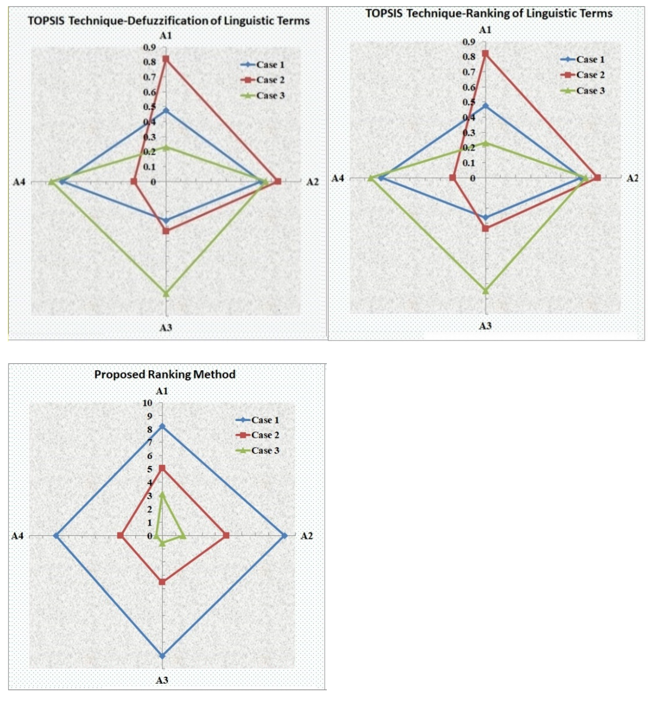
5.4. Comparison Study of the Proposed Ranking Method

This comparison study allowed us to see how effectively the proposed approach operated. Table 9 compares the results of our proposed ranking with those of various existing fuzziness results. The interval-type-2 fuzzy number was developed and contributed to by the authors Chen and L.W. Lee [57], Hu et al. [52], and Ilieva [53] to cope with uncertainty. To deal with the uncertainty, the generalization case of the IT2FS membership function had some limitations. Since Liu and Su’s method [55] and Wang and Luo’s method [56] dealt with the ranking of IT2FS to distinguish the preference order of the alternatives, Chen and Wang’s [51] methods addressed these drawbacks. However, there was a drawback of the ranking score function for solving the MCDM problem when we considered input as a linguistic term in the form of GIT2TrFN. We considered a new ranking of GIT2TrFN, and the defuzzification of GIT2TrFN helped to apply the TOPSIS–MCDM technique for numerical applications to overcome these shortcomings in existing methods. Table 9 shows the ranking order of sustainable transportation alternatives using the proposed ranking methods. Our proposed numerical example of the MCDM problem on sustainable transport was divided into case 1: Economic factors, case 2: Social factors, and case 3: Environmental factors. Here, we analyzed these cases with four alternatives and different criteria. In Table 9, Result 1 demonstrates that the proposed ranking approach did not use any MCDM technique, as per Section 3.1. However, Results 2 and 3 show that the TOPSIS technique was used, with the decision matrix ranking of linguistic terms and defuzzification of linguistic terms.

6. Sensitivity Analysis

This section discusses the sustainable transportation factors that impacted the decision, including the presented ranking results on alternatives for the suitable criteria. A sensitivity analysis was performed to acquire a better understanding of the impact of our proposed ranking method on the numerical example problem, which was divided into three cases by decision-makers: Case-1: Economic factors, Case-2: Social factors, and Case-3: Environmental factors. The ranking results were analyzed by plotting Figure 6, which shows how the results changed when different ranking results were considered with various alternatives.

Table 9. Comparison of ranking preferences with existing methods.

Authors/Methods	Fuzziness	Alternatives				Ranking Preference
		${\mathit{A}}_1$	${\mathit{A}}_2$	${\mathit{A}}_3$	${\mathit{A}}_4$
Chen & L.-W. Lee [56]	IT2FS	0.2481	0.2161	0.2181	-	$A_2\succ A_1\succ A_3$
Chen & Wang [51]	GTRFN	0.3311	0.4121	0.3906	-	$A_3\succ A_2\succ A_1$
Hu et al. [52]	IT2FN	0.2331	0.2523	0.2941	-	$A_2\succ A_1\succ A_3$
Celik et al. [58]	IT2TrFN	4.3345	5.9340	4.6345	-	$A_2\succ A_3\succ A_1$
Ilieva [53]	IT2FN	0.1201	0.2880	1.1905	0.1584	$A_3\succ A_2\succ A_4\succ A_1$
Result 1: Proposed Ranking Method
Case 1	GIT2TrFN	8.1993	9.1927	9.0270	7.9871	$A_1\succ A_3\succ A_1\succ A_4$
Case 2	GIT2TrFN	5.0451	4.8320	3.5132	3.1203	$A_1\succ A_2\succ A_3\succ A_4$
Case 3	GIT2TrFN	3.1101	1.5759	0.5713	0.4363	$A_1\succ A_2\succ A_3\succ A_4$
Result 2: TOPSIS Technique (Ranking of linguistic terms)
Case 1	GIT2TrFN	0.4744	0.6340	0.2620	0.6920	$A_4\succ A_2\succ A_1\succ A_3$
Case 2	GIT2TrFN	0.8176	0.7448	0.3361	0.2148	$A_1\succ A_2\succ A_3\succ A_4$
Case 3	GIT2TrFN	0.2310	0.6646	0.7454	0.7630	$A_4\succ A_3\succ A_2\succ A_1$
Result 3: TOPSIS Technique (Defuzzification of linguistic terms)
Case 1	GIT2TrFN	0.4739	0.6330	0.2611	0.6928	$A_4\succ A_2\succ A_1\succ A_3$
Case 2	GIT2TrFN	0.8185	0.7477	0.3335	0.2128	$A_1\succ A_2\succ A_3\succ A_4$
Case 3	GIT2TrFN	0.2306	0.6660	0.7481	0.7638	$A_4\succ A_3\succ A_2\succ A_1$

Table 9. Comparison of ranking preferences with existing methods.

Authors/Methods	Fuzziness	Alternatives				Ranking Preference
		${\mathit{A}}_1$	${\mathit{A}}_2$	${\mathit{A}}_3$	${\mathit{A}}_4$
Chen & L.-W. Lee [56]	IT2FS	0.2481	0.2161	0.2181	-	$A_2\succ A_1\succ A_3$
Chen & Wang [51]	GTRFN	0.3311	0.4121	0.3906	-	$A_3\succ A_2\succ A_1$
Hu et al. [52]	IT2FN	0.2331	0.2523	0.2941	-	$A_2\succ A_1\succ A_3$
Celik et al. [58]	IT2TrFN	4.3345	5.9340	4.6345	-	$A_2\succ A_3\succ A_1$
Ilieva [53]	IT2FN	0.1201	0.2880	1.1905	0.1584	$A_3\succ A_2\succ A_4\succ A_1$
Result 1: Proposed Ranking Method
Case 1	GIT2TrFN	8.1993	9.1927	9.0270	7.9871	$A_1\succ A_3\succ A_1\succ A_4$
Case 2	GIT2TrFN	5.0451	4.8320	3.5132	3.1203	$A_1\succ A_2\succ A_3\succ A_4$
Case 3	GIT2TrFN	3.1101	1.5759	0.5713	0.4363	$A_1\succ A_2\succ A_3\succ A_4$
Result 2: TOPSIS Technique (Ranking of linguistic terms)
Case 1	GIT2TrFN	0.4744	0.6340	0.2620	0.6920	$A_4\succ A_2\succ A_1\succ A_3$
Case 2	GIT2TrFN	0.8176	0.7448	0.3361	0.2148	$A_1\succ A_2\succ A_3\succ A_4$
Case 3	GIT2TrFN	0.2310	0.6646	0.7454	0.7630	$A_4\succ A_3\succ A_2\succ A_1$
Result 3: TOPSIS Technique (Defuzzification of linguistic terms)
Case 1	GIT2TrFN	0.4739	0.6330	0.2611	0.6928	$A_4\succ A_2\succ A_1\succ A_3$
Case 2	GIT2TrFN	0.8185	0.7477	0.3335	0.2128	$A_1\succ A_2\succ A_3\succ A_4$
Case 3	GIT2TrFN	0.2306	0.6660	0.7481	0.7638	$A_4\succ A_3\succ A_2\succ A_1$

In Table 9, regarding Result 2, and Result 3, the alternatives had the same ranking, based on outcomes of the proposed ranking results. That is, the ranking of GIT2TrFN linguistic terms and the defuzzification of GIT2TrFN linguistic representations resulted in the same effect when utilizing the TOPSIS technique. The components of environmentally responsible transportation could vary depending on the situation.

In terms of financial considerations, the alternatives were ordered as follows: $A_4\succ A_2\succ A_1\succ A_3$ based on the criterion speed (C₂). The criterion of Speed (C₂) played a significant role in the economic factors of ST. That is, people might choose speedy modes of transportation (such as A₄-plane Transportation) that have shorter travel periods and have less cost or energy to operate. Due to the accessibility of the criterion, the choices for the social aspects category were sorted as follows $A_1\succ A_2\succ A_3\succ A_4$. People always preferred a mode of transportation that was easily accessible (A₁-Road transportation), and the alternatives for environmental factors were ranked as follows: $A_4\succ A_3\succ A_2\succ A_1$. That is, in the environmental factors, pollution (C₁₂) was a significant criterion for ST. Environmental issues comprised not just one but four different types of pollution: air pollution, water pollution, soil contamination, and noise pollution. Pollution levels must be reduced to provide sustainable mobility. Figure 6 shows how the alternatives performed in terms of their ranking. The decision-making technique developed in this study collected information data offered by decision-makers using proposed ranking scores that correlated to different alternatives.

7. Conclusions

This paper presents an MCGDM approach for analyzing the viability of urban conveyance systems in an environment full of uncertainties. This work used a GIT2TrFN to reflect the imprecise nature of choice to deal with the uncertainty presented by the MCGDM problem. The proposed ranking approach generated innovative and unique outcomes concerning uncertainty in the MCGDM situations. The individuals making decisions could consider various transportation choices (A_i) and criteria (C_j). The MCGDM problem could be solved by applying the provided ranking functions to the coefficients and integers formatted as GIT2TrFNs. The proposed ranking functions translated IT2FNs into a clear number-based equivalent MCGDM issue that could be solved quickly. As a direct result of the ranking methods proposed for the GIT2TrFNs, it was not difficult to rank and compare the numerous individual cases of GIT2TrFN, which was accomplished with relative ease. The fact that the newly suggested way of ranking produced original and unheard-of outcomes proved that the method in question can be relied upon and is suitable for implementation.

Therefore, these methods provide solutions that may be put into practice for comparing type-1 and IT2FNs using fuzzy MCDM problems. These methods allow for the evaluation of intervals concerning type-2 fuzzy numbers. This research employed a GIT2TrFN to mirror the fuzziness of decision-making to cope with the unpredictability of outcomes associated with the MCGDM problem-solving process. Concerning the MCDM problems’ ambiguities in the criteria or alternatives, GIT2TrFN is a general attribute fuzzy system that works better for problem modeling. A more comprehensive range of detection options for uncertainty is possible. This is because there is more data available and greater complexity involved in a fuzzy system. A novel ranking approach, GIT2TrFN, was created to deal with the issues brought on by fuzzy MCGDM. By providing a ranking system for green transportation solutions, the system promotes more informed decision-making by people in power. To sum up, we divided eco-friendly modes of transportation into three main groups. The decision maker’s opinion was communicated linguistically by ranking the remaining options according to the significance of the criteria. Finally, we conclude that our proposed ranking approach simplifies the handling of linguistic terms as GIT2TrFNs. It is simple to use to handle any type of MCDM problem. The interval type-1 trapezoidal fuzzy number and GIT2TrFN are not completely equivalent. We can also apply this research to the similarity/symmetry approach of two GIT2TrFNs.

References

1. Cracolici, M.F.; Cuffaro, M.; Nijkamp, P. The Measurement of Economic, Social and Environmental Performance of Countries: A Novel Approach. Soc. Indic. Res. 2009, 95, 339–356. [Google Scholar] [CrossRef] [Green Version]
2. Ribeiro, P.; Fonseca, F.; Santos, P. Sustainability assessment of a bus system in a mid-sized municipality. J. Environ. Plan. Manag. 2020, 63, 236–256. [Google Scholar] [CrossRef]
3. Karjalainen, L.E.; Juhola, S. Framework for Assessing Public Transportation Sustainability in Planning and Policy-Making. Sustainability 2019, 11, 1028. [Google Scholar] [CrossRef] [Green Version]
4. Avineri, E.; Prashker, J.; Ceder, A. Transportation projects selection process using fuzzy sets theory. Fuzzy Sets Syst. 2000, 116, 35–47. [Google Scholar] [CrossRef]
5. Rajak, S.; Parthiban, P.; Dhanalakshmi, R. Sustainable transportation systems performance evaluation using fuzzy logic. Ecol. Indic. 2016, 71, 503–513. [Google Scholar] [CrossRef]
6. Hansson, J.; Pettersson, F.; Svensson, H.; Wretstrand, A. Preferences in regional public transport: A literature review. Eur. Transp. Res. Rev. 2019, 11, 38. [Google Scholar] [CrossRef] [Green Version]
7. Stefaniec, A.; Hosseini, K.; Assani, S.; Hosseini, S.M.; Li, Y. Social sustainability of regional transportation: An assessment framework with application to EU road transport. Socio-Econ. Plan. Sci. 2021, 78, 101088. [Google Scholar] [CrossRef]
8. Liang, H.; Ren, J.; Lin, R.; Liu, Y. Alternative-fuel based vehicles for sustainable transportation: A fuzzy group decision supporting framework for sustainability prioritization. Technol. Forecast. Soc. Chang. 2019, 140, 33–43. [Google Scholar] [CrossRef]
9. Gupta, M. A Fuzzy Decision-making Approach to Evaluate CO2 Emissions Reduction Policies. Glob. Bus. Rev. 2021. [Google Scholar] [CrossRef]
10. Kennedy, C.A. A comparison of the sustainability of public and private transportation systems: Study of the Greater Toronto Area. Transportation 2002, 29, 459–493. [Google Scholar] [CrossRef]
11. Pamucar, D.; Ecer, F.; Deveci, M. Assessment of alternative fuel vehicles for sustainable road transportation of United States using integrated fuzzy FUCOM and neutrosophic fuzzy MARCOS methodology. Sci. Total. Environ. 2021, 788, 147763. [Google Scholar] [CrossRef]
12. Lv, T.; Wang, Y.; Deng, X.; Zhan, H.; Siskova, M. Sustainability transition evaluation of urban transportation using fuzzy logic method-the case of Jiangsu Province. J. Intell. Fuzzy Syst. 2020, 39, 3883–3898. [Google Scholar] [CrossRef]
13. Agrawal, V.; Seth, N.; Dixit, J.K. A combined AHP–TOPSIS–DEMATEL approach for evaluating success factors of e-service quality: An experience from Indian banking industry. Electron. Commer. Res. 2020, 22, 715–747. [Google Scholar] [CrossRef]
14. Yedla, S.; Shrestha, R.M. Multi-criteria approach for the selection of alternative options for environmentally sustainable transport system in Delhi. Transp. Res. Part A Policy Pract. 2003, 37, 717–729. [Google Scholar] [CrossRef]
15. Awasthi, A.; Chauhan, S.S.; Omrani, H. Application of fuzzy TOPSIS in evaluating sustainable transportation systems. Expert Syst. Appl. 2011, 38, 12270–12280. [Google Scholar] [CrossRef]
16. Rossi, R.; Gastaldi, M.; Gecchele, G. Sustainability evaluation of transportation policies: A fuzzy-based method in a “what to” analysis. Adv. Intell. Syst. Comput. 2014, 223, 315–326. [Google Scholar]
17. Wei, H.-H.; Liu, M.; Skibniewski, M.J.; Balali, V. Prioritizing sustainable transport projects through multi-criteria group decision making: Numerical example of Tianjin Binhai new area, China. J. Manag. Eng. 2016, 32, 04016010. [Google Scholar] [CrossRef]
18. Mardani, A.; Zavadskas, E.K.; Khalifah, Z.; Jusoh, A.; Nor, K. Multiple criteria decision-making techniques in transportation systems: A systematic review of the state of the art literature. Transport 2016, 31, 359–385. [Google Scholar] [CrossRef] [Green Version]
19. Deveci, M.; Canıtez, F.; Gökaşar, I. WASPAS and TOPSIS based interval type-2 fuzzy MCDM method for a selection of a car sharing station. Sustain. Cities Soc. 2018, 41, 777–791. [Google Scholar] [CrossRef]
20. Shankar, R.; Choudhary, D.; Jharkharia, S. An integrated risk assessment model: A case of sustainable freight transportation systems. Transp. Res. Part D Transp. Environ. 2018, 63, 662–676. [Google Scholar] [CrossRef]
21. Tan, Y.; Shuai, C.; Jiao, L.; Shen, L. Adaptive neuro-fuzzy inference system approach for urban sustainability assessment: A China numerical example. Sustain. Dev. 2018, 26, 749–764. [Google Scholar] [CrossRef]
22. Büyüközkan, G.; Feyzioğlu, O.; Göçer, F. Selection of sustainable urban transportation alternatives using an integrated intuitionistic fuzzy Choquet integral approach. Transp. Res. Part D Transp. Environ. 2018, 58, 186–207. [Google Scholar] [CrossRef]
23. Moslem, S.; Ghorbanzadeh, O.; Blaschke, T.; Duleba, S. Analyzing stakeholder consensus for a sustainable transport development decision by the fuzzy AHP and interval AHP. Sustainability 2019, 11, 3271. [Google Scholar] [CrossRef] [Green Version]
24. Kumar, A.; Singh, G.; Vaidya, O.S. A comparative evaluation of public road transportation systems in india using multi-criteria decision-making techniques. J. Adv. Transp. 2020, 2020, 8827186. [Google Scholar] [CrossRef]
25. Svadlenka, L.; Simic, V.; Dobrodolac, M.; Lazarevic, D.; Todorovic, G. Picture Fuzzy Decision-Making Approach for Sustainable Last-Mile Delivery. IEEE Access 2020, 8, 209393–209414. [Google Scholar] [CrossRef]
26. Yannis, G.; Kopsacheili, A.; Dragomanovits, A.; Petraki, V. State-of-the-art review on multi-criteria decision-making in the transport sector. J. Traffic Transp. Eng. (Engl. Ed.) 2020, 7, 413–431. [Google Scholar] [CrossRef]
27. Singh, S.; Agrawal, V.; Mohanty, R. Multi-criteria decision analysis of significant enablersfor a competitive supply chain. J. Adv. Manag. Res. 2022, 19, 414–442. [Google Scholar] [CrossRef]
28. Hamurcu, M.; Eren, T. Electric bus selection with multi-criteria decision analysis for green transportation. Sustainability 2020, 12, 2777. [Google Scholar] [CrossRef] [Green Version]
29. Marimuthu, D.; Mahapatra, G.S. Multi-criteria decision-making using a complete ranking of generalized trapezoidal fuzzy numbers. Soft Comput. 2021, 25, 9859–9871. [Google Scholar] [CrossRef]
30. Keshavarz-Ghorabaee, M.; Amiri, M.; Hashemi-Tabatabaei, M.; Ghahremanloo, M. Sustainable Public Transportation Evaluation using a Novel Hybrid Method Based on Fuzzy BWM and MABAC. Open Transp. J. 2021, 15, 31–46. [Google Scholar] [CrossRef]
31. Sharma, V. Multi-objective optimization in hard turning of tool steel using integration of taguchitopsis under wet conditions. Int. J. Eng. Trends Technol. 2020, 68, 37–41. [Google Scholar] [CrossRef]
32. Ziemba, P. Selection of electric vehicles for the needs of sustainable transport under conditions of uncertainty—A comparative study on fuzzy MCDA methods. Energies 2021, 14, 7786. [Google Scholar] [CrossRef]
33. Romero-Ania, A.; Rivero Gutiérrez, L.; De Vicente Oliva, M.A. Multiple Criteria Decision Analysis of Sustainable Urban Public Transport Systems. Mathematics 2021, 9, 1844. [Google Scholar] [CrossRef]
34. Broniewicz, E.; Ogrodnik, K. A Comparative Evaluation of Multi-Criteria Analysis Methods for Sustainable Transport. Energies 2021, 14, 5100. [Google Scholar] [CrossRef]
35. Gutierrez, L.R.; Oliva, M.A.d.; Romero-Ania, A. Managing sustainable urban public transport systems: An AHP multi-criteria decision model. Sustainability 2021, 13, 4614. [Google Scholar] [CrossRef]
36. Agrawal, V.; Mohanty, R.; Agarwal, S.; Dixit, J.; Agrawal, A. Analyzing critical success factorsfor sustainable green supply chain management. Environ. Dev. Sustain. 2022. [Google Scholar] [CrossRef]
37. Lazaroiu, G.C.; Roscia, M. Fuzzy Logic Strategy for Priority Control of Electric Vehicle Charging. IEEE Trans. Intell. Transp. Syst. 2022, 23, 19236–19245. [Google Scholar] [CrossRef]
38. Anand, S.; Choudhary, A.; Singhal, P. Car ecoleasing encouraging product service system with circular economy to help environment. Indian J. Environ. Prot. 2019, 39, 352–358. [Google Scholar]
39. Tirkolaee, E.B.; Aydin, N.S. Integrated design of sustainable supply chain and transportation network using a fuzzy bi-level decision support system for perishable products. Expert Systems Appl. 2022, 195, 116628. [Google Scholar] [CrossRef]
40. Demir, G.; Damjanovic, M.; Matovic, B.; Vujadinovic, R. Toward sustainable urban mobility by using fuzzy-fucom and fuzzy-cocoso methods: The case of the SUMP Podgorica. Sustainability 2022, 14, 4972. [Google Scholar] [CrossRef]
41. Goyal, S.; Garg, D.; Luthra, S. Sustainable production and consumption: Analyzing barriers and solutions for maintaining green tomorrow by using fuzzy-AHP–fuzzy-TOPSIS hybrid framework. Environ. Dev. Sustain. 2021, 23, 16934–16980. [Google Scholar] [CrossRef]
42. Xu, J.; Song, R.; Zhu, H. Evaluation of Smart City Sustainable Development Prospects Based on Fuzzy Comprehensive Evaluation Method. Comput. Intell. Neurosci. 2022, 2022, 5744415. [Google Scholar] [CrossRef]
43. Pérez, J.C.; Carrillo, M.H.; Montoya-Torres, J.R. Multi-criteria approaches for urban passenger transport systems: A literature review. Ann. Oper. Res. 2015, 226, 69–87. [Google Scholar] [CrossRef]
44. Pamucar, D.; Deveci, M.; Canıtez, F.; Paksoy, T.; Lukovac, V. A Novel Methodology for Prioritizing Zero-Carbon Measures for Sustainable Transport. Sustain. Prod. Consum. 2021, 27, 1093–1112. [Google Scholar] [CrossRef]
45. Bakioglu, G.; Atahan, A.O. AHP integrated TOPSIS and VIKOR methods with Pythagorean fuzzy sets to prioritize risks in self-driving vehicles. Appl. Soft Comput. 2021, 99, 106948. [Google Scholar] [CrossRef]
46. Zarbakhshnia, N.; Soleimani, H.; Ghaderi, H. Sustainable third-party reverse logistics provider evaluation and selection using fuzzy SWARA and developed fuzzy COPRAS in the presence of risk criteria. Appl. Soft Comput. 2018, 65, 307–319. [Google Scholar] [CrossRef]
47. Yang, C.; Wang, Q.; Pan, M.; Hu, J.; Peng, W.; Zhang, J.; Zhang, L. A linguistic Pythagorean hesitant fuzzy MULTIMOORA method for third-party reverse logistics provider selection of electric vehicle power battery recycling. Expert Syst. Appl. 2022, 198, 116808. [Google Scholar] [CrossRef]
48. Hajduk, S. Multi-Criteria Analysis in the Decision-Making Approach for the Linear Ordering of Urban Transport Based on TOPSIS Technique. Energies 2022, 15, 274. [Google Scholar] [CrossRef]
49. Hwang, C.L.; Yoon, K. Methods for Multiple Attribute Decision Making. In Multiple Attribute Decision Making; Springer: Berlin/Heidelberg, Germany, 1981; pp. 58–191. [Google Scholar]
50. Hwang, C.-L.; Lai, Y.-J.; Liu, T.-Y. A new approach for multiple objective decision making. Comput. Oper. Res. 1993, 20, 889–899. [Google Scholar] [CrossRef]
51. Chen, S.-M.; Wang, C.-Y. Fuzzy decision making systems based on interval type-2 fuzzy sets. Inf. Sci. 2013, 242, 1–21. [Google Scholar] [CrossRef]
52. Hu, J.; Zhang, Y.; Chen, X.; Liu, Y. Multi-criteria decision making method based on possibility degree of interval type-2 fuzzy number. Knowl.-Based Syst. 2013, 43, 21–29. [Google Scholar] [CrossRef]
53. Ilieva, G. Group Decision Analysis with Interval Type-2 Fuzzy Numbers. Cybern. Inf. Technol. 2017, 17, 31–44. [Google Scholar] [CrossRef]
54. Meniz, B. An advanced TOPSIS method with new fuzzy metric based on interval type-2 fuzzy sets. Expert Syst. Appl. 2021, 186, 115770. [Google Scholar] [CrossRef]
55. Liu, P.; Su, Y. Multiple attribute decision-making method based on the trapezoid fuzzy linguistic hybrid harmonic averaging operator. Informatica 2012, 36, 83–90. [Google Scholar]
56. Wang, Y.-M.; Luo, Y. Area ranking of fuzzy numbers based on positive and negative ideal points. Comput. Math. Appl. 2009, 58, 1769–1779. [Google Scholar] [CrossRef] [Green Version]
57. Chen, S.-M.; Lee, L.-W. Fuzzy multiple attributes group decision-making based on the ranking values and the arithmetic operations of interval type-2 fuzzy sets. Expert Syst. Appl. 2010, 37, 824–833. [Google Scholar] [CrossRef]
58. Celik, E.; Bilisik, O.N.; Erdogan, M.; Gumus, A.T.; Baracli, H. An integrated novel interval type-2 fuzzy MCDM method to improve customer satisfaction in public transportation for Istanbul. Transp. Res. Part E Logist. Transp. Rev. 2013, 58, 28–51. [Google Scholar] [CrossRef]
59. Türkşen, I. Type 2 representation and reasoning for CWW. Fuzzy Sets Syst. 2002, 127, 17–36. [Google Scholar] [CrossRef]
60. Wang, Y.-J.; Lee, H.-S. The revised method of ranking fuzzy numbers with an area between the centroid and original points. Comput. Math. Appl. 2008, 55, 2033–2042. [Google Scholar] [CrossRef] [Green Version]
61. Yager, R.R. Fuzzy subsets of type-2 in decisions. J. Cybern. 1980, 10, 137–159. [Google Scholar] [CrossRef]
Figure 1. Sustainable transport articles using fuzzy-based decision techniques for the period 2000–2022.
Mathematics 10 04534 g001
Figure 2. Sustainable transportation articles using decision-making techniques for the period 2000–2022.
Mathematics 10 04534 g002
Figure 3. Sustainable transportation articles of a fuzzy nature for the period 2000–2022.
Mathematics 10 04534 g003
Figure 4. Representation of GIT2TrFN.
Mathematics 10 04534 g004
Figure 5. Leading scenarios and attributes for sustainable transportation.
Mathematics 10 04534 g005
Figure 6. Ranking Performance for presented three cases.
Mathematics 10 04534 g006