Abstract
The two-dimensional, time-independent conjugate natural convection flow and entropy generation are numerically investigated in three different cases of a wavy conducting solid block attached to the left wall of a square cavity. A hybrid nanofluid with titania (TiO2) and copper (Cu) nanoparticles and base fluid water in the fluid part is considered in the presence of a uniform inclined magnetic field. The leftmost wall of the cavity is the hot one and the rightmost one is the cold one. Radial-basis-function-based finite difference (RBF-FD) is performed on an appropriate designed grid distribution. Numerical results in view of streamlines and isotherms, as well as average Nusselt number in an interface and total entropy generation are presented. The related parameters such as Hartmann number, Rayleigh number, conductivity ratio, amplitude in wavy wall, number of waviness, and inclination angle of magnetic field are observed. Convective heat transfer in the fluid part is an increasing function of , while it deflates with the rise in in each case. Total entropy generation increases with the increase in and but it decreases with values. Average Bejan number ascends with the rise in and descends with the rise in .
Keywords:
wavy conducting solid; conjugate natural convection flow; Cu-TiO2/water; radial basis functions; entropy generation MSC:
76R10; 35Q35; 76M22; 80M22; 28D20
1. Introduction
In recent years, there have been many studies on heat transfer (HT) and fluid flow (FF) in enclosures in the presence of different combinations of porous medium, mono and hybrid nanoparticles, bacteria, conducting bodies, and magnetic fields (MF). The main objective in each of these studies is to observe the HT enhancement. The influence of nanoparticles on HT improvement was initially shown by Choi et al. [1]. Since then, many numerical and experimental studies may be found on nanofluids (NF).
Kasaeipoor et al. [2] performed a numerical study by using the Lattice Boltzmann method (LBM) to investigate the entropy generation (EG) due to buoyancy-induced flow in a closed space with refrigerant solid and hybrid NFs. They also made a work to measure the thermophysical properties of the nanofluid MWCNT-MgO (15–85%)/Water. They showed that the configuration of refrigerant rigid body pronounced the effect on EG. Hybrid NFs are used for different HT applications such as solar collectors and radiators in literature due to the controllable viscosity, density, thermal conductivity, and specific heat. These applications are reviewed by Huminic and Huminic [3]. Another review has been performed on HT enhancement techniques using hybrid NFs by Muneeshwaran et al. [4]. Dutta et al. [5] studied the impact of hybrid nanoparticles on conjugate mixed convection (MC) of a viscoplastic fluid in a ventilated enclosure. A hybrid NF enhances the HT and EG with the rate of HT higher than the rate of EG. Zhang et al. [6] performed a study on conjugate buoyant heat transport in NFs with different nanoparticles. They formulated the generalized Cattaneo law of thermal flux with analytical methods. They found that the heat flux given by the fractional equation leads to the decrease in HT in the solid wall. Priam et al. [7] studied conjugate natural convection (NC) in a vertically divided square-shaped closed space with a corrugated solid partition into air and water regions. They showed that increasing the partition thermal conductivity enhances the thermal performance by up to 25%. Conjugate unsteady NC of air and non-Newtonian fluid in a thick-walled cylindrical closed space partially filled with a porous media was studied by Rodríguez-Núñez et al. [8]. They used finite-volume method (FVM) to solve governing equations. The effects of internal heat generation or absorption on conjugate thermal-NC of a suspension of hybrid NF in a partitioned circular annulus are analyzed by Tayebi et al. [9]. They proposed a new correlation on the mean heat exchange rate in the defined parameters.Entropy generation is an important issue for almost all energy system applications. EG is reviewed in the literature [10] for NC and MC HT. Mondal and Mahapatra [11] solved a numerical problem on magnetohydrodynamics (MHD) double-diffusive MC and EG of NF in a trapezoidal shaped closed space considering the effects of MF. They used the second- and the fourth-order finite difference (FD) approximations to solve the governing equations, and their results show that low MF and low aspect ratio are always preferable to reduce total EG. Korei et al. [12] performed a study on the combined convection and irreversibility analysis under MF for hybrid NF in a partially heated lid-driven enclosure. They used OpenFOAM with a C++ open-source code. They found that the combination of Al2O3 75% and Cu 25% give the highest values of the mean Nusselt (Nu) number and the entropy production. Tayebi et al. [13] performed a study on NC and EG of hybrid-nanoliquid-filled annulus delimited by two elliptic cylinders. Their results showed that hybrid nanoliquid significantly alters the hydrothermal characteristics and EG. Ahrar et al. [14] performed a numerical analysis of NF HT and EG in a closed space by using a novel total variation diminishing hybrid LBM under the MF. They showed that EG can be controlled via MF. Majeed et al. [15] solved the problem of EG in a hexagonally shaped closed space with magnetized hybrid nanomaterials. They used FEM, and their results report that increasing MF’s effects reduces the HT since the conduction motion occupies the motion of the FF. Priyadharsini and Sivaraj [16] studied the entropy production in a ferrofluid filled square closed space with a solid body generating inner heat. They showed that minimum entropy production occurs at the lowest thermal conductivity value. Sachica et al. [17] solved an MHD MC and EG problem by using vorticity, and the stream function form coupled with the energy equation is solved using the control volume method on a nonuniform orthogonal Cartesian grid. They found that the EG is dominated by irreversibilities due to HT for all values of the nanoparticle volume fraction. Inclined magneto-conjugate HT and EG in an inclined domain with a wavy partition are analyzed by Priam and Nasrin [18]. They used FEM and observed that thermal performance and EG are significantly influenced by the MF intensity and closed space inclination. The two-phase mixture model is used to assess the effects of the nanoparticle shape on the hydrothermal aspects and EG of turbulent convection of NF by Alsarraf et al. [19], applying the problem to flat plate solar collector. They examined EG corresponding to different cases and a flow rate. Varol et al. [20] performed a study on the EG due to the conjugate NC in a thick-walled closed space by using FDM for different parameters. Their results demonstrate that EG increases with increasing thermal conductivity ratio and thickness of the walls. EG due to NC in a partially heated triangular closed space was investigated by Varol et al. [21] utilizing FDM. They observed that EG increases but Bejan (Be) number decreases with increasing Ra number. In their other work in [22], they solved the problem of EG for conjugate trapezoid-shaped closed space. They showed that the most important parameters affecting HT and FF are thermal conductivity ratio and dimensionless thickness of the solid wall of the closed space. The conjugate NC flow of SiO2-water nanofluid in the presence of oxytactic bacteria, periodic magnetic field, and Brownian and Thermophoresis effects is studied in [23]. The results show that convective HT is an increasing function of conductivity ratio. The EG and convection effect on magnetized hybrid nano-liquid flow inside a trapezoidal closed space with a zigzagged wall is studied in [24] and nano-encapsulated phase change particles in a semi-annular cavity in [25]. Magherbi et al. [26] observed HT and FF irreversibilities on unsteady NC flow, utilizing a control-volume finite element method (FEM). In their results, FF irreversibility dominates over HT irreversibility as the Rayleigh () number rises. Ilis et al. [27] examined total EG in the case of different aspect ratios, performing alternating-direction implicit scheme. They reported that total EG increases with the increase in . A similar aspect ratio analysis is noted in Oliveski et al. [28] using FVM. Parvin et al. [29] implemented FEM for the simulation of NC of Cu–water NF in an odd-shaped cavity while taking EG into account. Their results reveal that HT irreversibility rises with the increase in . Pordanjani et al. [30] studied the radiation effect on NC and EG in a diagonal rectangular cavity involving an NF in the presence of a uniform MF. They concluded that EG increases with increasing radiation parameter.
In the current study, the conjugate (convection and conduction) natural convection flow and entropy generation of a hybrid NF, TiO2-Cu/water, in an enclosure with a wavy conducting solid block is numerically investigated in the presence of an inclined uniform MF. To the best of the authors’ knowledge, the wavy conducting solid part is taken into account for the first time. Numerical results are obtained by performing an in-house implementation of the radial-basis-function-based finite difference method.
2. Problem Formulation
The two dimensional, time-independent natural convection flow in an enclosure involving wavy conducting solid block attached to the left wall is considered. The leftmost wall is the hot wall, while the right vertical straight wall is the cold wall in the enclosure sketched in Figure 1. The top and the bottom walls are adiabatic, where . Hybrid NF TiO2-Cu/water exists in the fluid part, while the the solid part of size is thermally conducting. The enclosure is also exposed to a uniform MF with an inclination angle . It is assumed that the nanofluid is Newtonian, the flow is laminar and incompressible, and thermal equilibrium exists between nanoparticles and the base fluid. Induced MF, viscous dissipation, Joule heating, and radiation effects are neglected.
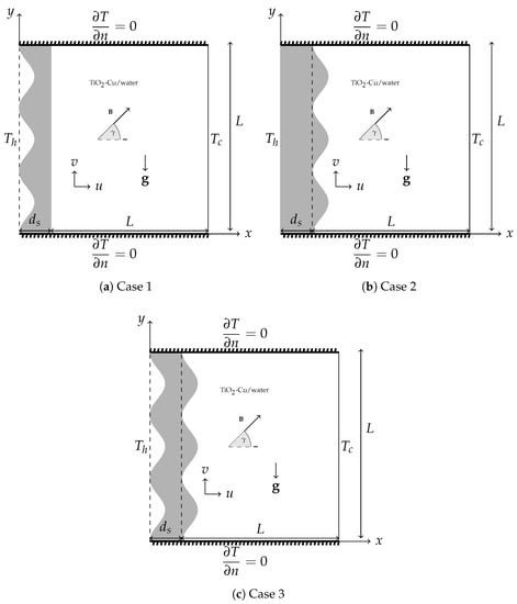
Figure 1.
Configuration of the flow, problem geometry and coordinates. B = .
Bearing in mind the single-phase NF model, some physical relations for NF may be listed as
where and subindices refer to the host fluid, nanoparticle and hybrid NF, respectively; is the density; is the specific heat at constant pressure; is the thermal expansion coefficient; is the dynamic viscosity (modelled by Brinkman’s model [31]); k is the thermal conductivity; and is the electrical conductivity ( and models are based on Maxwell’s model [32]).
Density variation due to the buoyancy force is treated with Bousinessq approximation. The other thermal and physical properties of water and nanoparticles are constant and are given in Table 1.

Table 1.
Physical Properties of Water and Nanoparticles [33].
Regarding the assumptions, the governing dimensional equations as a combination of continuity equation, momentum equations, and energy equation are as follows [21,30]:
where are the velocity components, p is the pressure, g is the gravitational acceleration, is the thermal diffusivity of hybrid NF, and subindex s refers to the solid.
In order to derive dimensionless equations, the following dimensionless variables are introduced [34]
where L is the characteristic length, . These variables are put into the dimensional equations, and then the prime notations are dropped. In the obtained form, elimination of pressure terms are also done by employing the definition of vorticity in the momentum equations. Velocity components in terms of stream function as satisfy the continuity equation. Thus, dimensionless equations in stream function-vorticity form are
where Prandtl (), Rayleigh () and Hartmann () numbers are
On the boundary of the the fluid part, velocity of the fluid is zero, as is stream function, and vorticity is computed using its definition . For the boundary of the temperature in the entire region, on the leftmost wall, while the right wall is the cold wall . In the interface, temperature condition is carried out as , where is the thermal conductivity ratio. The normal gradient of temperature on the top and bottom adiabatic walls is zero.
3. Solution Method
Many researchers have been interested in radial basis functions (RBFs) in recent years because of the dependence of the discretization on the radial distance between points in the considered domain. Novel books [35,36] involve very useful details on RBFs in terms of both theoretical and applied approaches.
As a local method, RBF-FD provides localization using stencils. The paper Flyer et al. [37] explains the method very well. A brief explanation may be written as follows:
Let be a point with coordinates in the concerned domain . Let be a stencil centered at involving number of points around . In this stencil, the conventional RBF interpolation augmented with polynomial terms is expressed as
subject to the constraints
where is an RBF depending on the radial distance with , and m is the total number of augmented polynomial terms.
In an equivalent matrix-vector form, Equation (6) may be written as
in which is the vector involving the terms , and is a matrix of size involving RBF matrix constructed by with nodes in a stencil and m additional polynomial terms added as rows and columns.
Cardinal basis functions are used to express the interpolant in another way as
where , and the cardinal basis function is defined as .
If is known, interpolation at a point will be as
where .
Combining Equations (9) and (10), is found as
where is a vector of size , but the last m terms are not used. Derivatives of this allow us to obtain differentiation matrices.
The steps of the current in-house implementation may be given as
- Nodes lying in a stencil centered at a node are determined. Let these nodes be denoted by .
- are shifted and centered as described in [37]. Then, a scaling in is performed with as introduced by Tominec [38]. Another useful scaling is also mentioned in [39].
- In stencil, using a polyharmonic spline RBF, , and cubic augmented polynomial terms matrix, is built.
- or (for x-derivatives) or (for y-derivatives) or (for Laplacian)) is found, and its first terms are saved. Note that scaling also affects and . Therefore, the differentiation matrices and are constructed by the first terms of .
Thus, the iterative solution of the dimensionless nonlinear governing equations is performed as follows:
where M is the matrix equal to , d stands for diagonal, and n is the iteration level.
For stream function and vorticity equations, only the matrices , and constructed in the fluid part are used. For temperature equations, these matrices are constructed in fluid and solid regions separately and are combined, keeping in mind the flux conditions at the interface.
Vorticity boundary conditions are achieved by using the definition of vorticity:
The iteration is terminated if
in which is the tolerance.
A parameter in interval eases the vorticity equation once it is solved as
Average Nu number along the interface separating the solid and the fluid part is calculated as
where s is the length of the interface.
In the fluid part, local HT irreversibility and local fluid friction irreversibility are adopted as [40]
endroup where is the irreversibility ratio held as and is the local Bejan number. Note that and in turn are obtained as vectors in the entire domain. In other words, we have discrete data for and . Average entropy over the entire two-dimensional domain is computed by using the double integral as
This double integral is calculated by using these discrete data cumulatively as introduced in ‘cumtrapz’ in Matlab’s library. In this study, composite Simpson’s rule is applied based on the idea expressed in ‘cumtrapz’. As a note, statistical mean for number defined by also gives very close results to this double integral result for . corresponds to the domination by HTI.
4. Numerical Outputs
4.1. Validation
In order to validate the current implemented code, some published problems are solved. Firstly, the basic unsteady benchmark problem as natural convection flow of air in a square cavity is considered using uniform nodes with RBF-FD in space derivatives and the Backward-Euler method in time derivatives.The obtained average Nu numbers along the heated left vertical wall are compared with the results in Reference [41]. As seen in Table 2, our results are in good agreement.
Table 2.
Comparison of average Nu numbers in a NC flow problem in a square cavity.
Secondly, the steady NC flow of a NF in a wavy cavity is considered, and average Nu values are compared in Table 3 in the case of a zero inclination angle of cavity, 0.05 solid volume fraction, and 0.05 amplitude of waviness in wavy walls. The grid points are arranged for that geometry. In the reference study, Ansys is utilized.
Table 3.
Comparison of average Nu values in the case of NC flow of an NF in a wavy cavity.
The third validation is to compare total EG contours of in different Rayleigh numbers when the irreversibility ratio is . As is seen in Figure 2, our results are in good agreement with Reference [26].
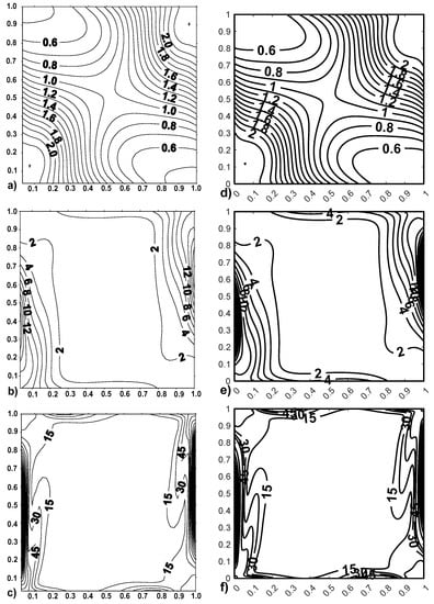
Figure 2.
Comparison of total entropy contours in a NC flow problem. (a–c) Reference [26] (the left); (d–f) Present (the right with ).
4.2. Grid Independency
Grid distributions for each case are designed as shown in Figure 3.
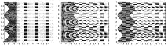
Figure 3.
Design of grid distribution. The (left) is for Case 1, the (middle) is for Case 2 and the (right) is for Case 3.
Grid independence is checked in Table 4. In all computations, , which means nodes, are used in all computations.
Table 4.
Grid independence analysis with .
4.3. Discussion on the Current Problem
In this part, numerical results are visualized as streamlines () and temperature (T) contours, as well as some graphs involving and EG parameters. The fixed parameters at all calculations are . The other pertinent parameter ranges are . In contours of , the given numbers almost at the center stand for values.
Figure 4 shows the behavior of FF and HT in various values of . The dampening effect of Lorentz force at large numbers is expected. This is verified from the decreasing values of . Further, MF comes along the hot wall horizontally at an angle . Therefore, the primary cell, particularly in Case 2 and 3, tends to be separated into new cells in large numbers. Isotherms almost exhibit conductive behavior at . That is, convection is suppressed by large Lorentz force.
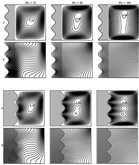
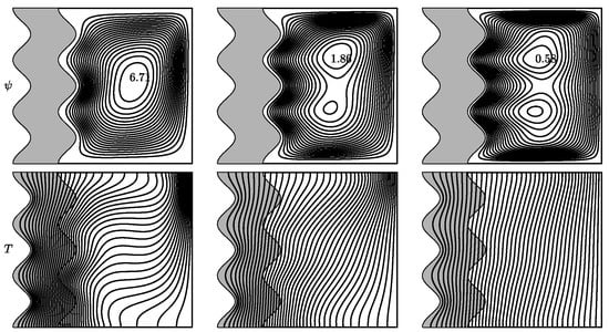
Figure 4.
Variation in when . Streamlines and isotherms at the (top) is for case 1, at the (middle) is for case 2 and the at (bottom) is for case 3.
Figure 5 illustrates the variation in number in three cases. In each cases, maximum absolute stream function values increases with the rise in number due to the increase in buoyancy force inside the fluid part. The core vortex in the primary cell in streamlines becomes smaller at , pointing to a faster fluid flow. The smallest values of when comparing each case are noted in Case 2. This may be due to the inhibition as a result of the larger area of the conductive solid block in Case 2 than in other cases. While isotherms exhibit a conductive behavior at , free convection behavior at is noted with a pronounced thermal gradient on the right vertical wall. On the contrary, increasing Rayleigh number does not make an important change in the solid wall.
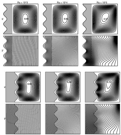
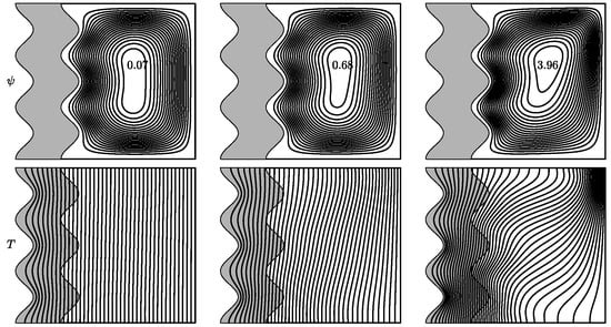
Figure 5.
Variation in when . Streamlines and isotherms at the (top) is for case 1, at the (middle) is for case 2 and the at (bottom) is for case 3.
The change in conductivity ratio is given in Figure 6. In all cases, the rise in causes fluid to flow faster, which is noted from the absolute maximum stream function values. Once again, the smallest values are obtained in Case 2. Since is directly proportional to , it is expected that conduction in the solid part should increase at . It is seen in isotherms at , in which no convective behavior occurs inside the solid part, while convection is clearly noted at . At , isotherms significantly cover the solid block, and these become rare in the fluid part. Furthermore, fluid flows faster as rises since the convective behavior in the fluid part becomes prominent due to the increase in .
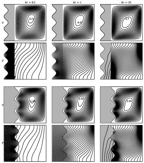
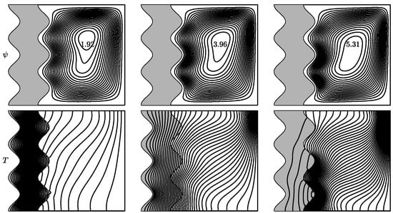
Figure 6.
Variation in when . Streamlines and isotherms at the (top) is for case 1, at the (middle) is for case 2 and the at (bottom) is for case 3.
The influence of amplitude of waviness is examined in Figure 7. In Case 1, increases with the increase in A. This may be due to the fact that more heat along the wavy wall in Case 1 is transferred to the fluid part, which makes the fluid flow faster. However, in Cases 2 and 3, a decrease in fluid velocity is noticed with the rise in A. This may be due to the smaller area of fluid part as a result of larger A.
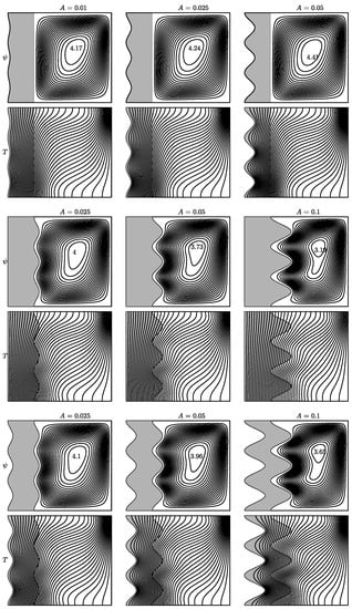
Figure 7.
Variation in A when . Streamlines and isotherms at the (top) is for case 1, at the (middle) is for case 2 and the at (bottom) is for case 3.
The impact of the number of waves in wavy wall is checked in Figure 8. In Case 1, stays almost the same in each n. In Cases 2 and 3, as n changes from 1 to 2, faster fluid flow is found, and then declines from to . However, compared to , fluid flows more rapidly when . Further, the smallest valuesof at any n are noted in Case 2 due to the larger area of conducting solid block than the other cases. If values in Case 1 and 3 are compared, not only the left wavy wall but also the waviness in the interface reduce the fluid velocity. That is, the hinderance in fluid flow increases with the rise in waviness. Convective behavior in isotherms in these two cases also become a bit more remarkable at than .
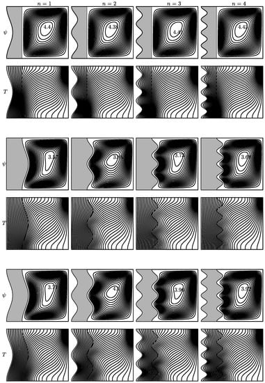
Figure 8.
Variation in n when . Streamlines and isotherms at the (top) is for case 1, at the (middle) is for case 2 and the at (bottom) is for case 3.
Figure 9 presents the variation in inclination angle of uniform MF. In Case 1, the angle has a significant effect on , which means that a quicker flow is noted in the flow part. Furthermore, the core vortex tends to obey the direction of the magnetic field. In Cases 2 and 3, ascends with the augmentation in the inclination angle of the MF, and isotherms are also more perturbed with this increment in angle . In other words, the flow can be controlled via a inclination angle of the MF.
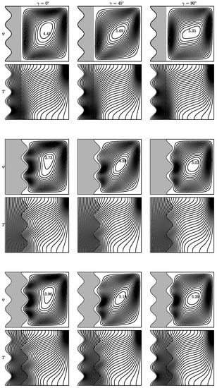
Figure 9.
Variation in when . Streamlines and isotherms at the (top) is for case 1, at the (middle) is for case 2 and the at (bottom) is for case 3.
Figure 10 shows the average Nu number along the interface, general EG, and average Bejan number in the variation in pertinent parameters. These outcomes are interpreted on the fluid part. In (a), escalates with the rise in number. That is, the convective heat transfer (CHT) rises in the fluid part. also rises with this increment in due to the rise in both HT and fluid friction irreversibilities. A reverse behavior is noted in the number.
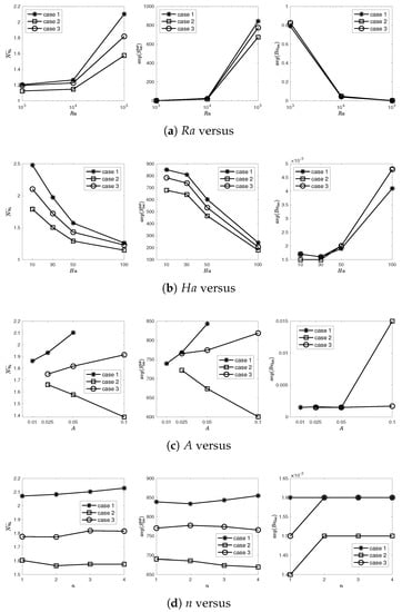
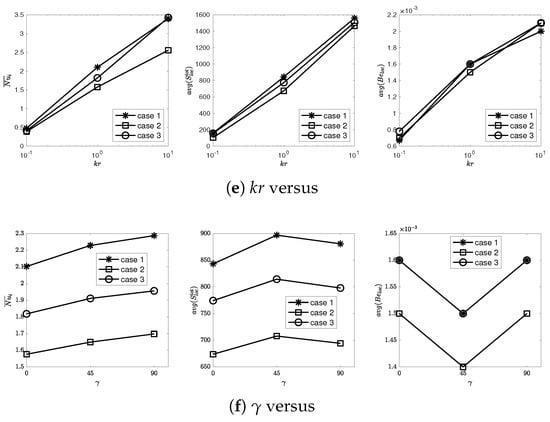
Figure 10.
graphs in different variations.
In (b), the rise in number weakens the CHT due to the dampening effect of the large Lorentz force. is also significantly reduced while the Bejan number rises. The reduction occurs the most in Case 3.
In (c), the augmentation in amplitude of the wavy wall affects the CHT in an increasing trend in Case 1 and 2 and a decreasing trend in Case 3. The same trend is exhibited in . Remember that Case 1 and 2 only had one wavy wall on the conducting solid, while the other vertical wall on the solid was straight. Therefore, it may be concluded that the wavy conducting block with a large amplitude has a reducing impact on CHT in FF.
In (d), the increment in the number of undulations has a rising influence on CHT and in Case 1. In Case 2 and Case 3, there is a rise and reduction behavior with the change in n. However, looking at the discrete data, CHT is efficient at in Case 3 and at in Case 2. In Case 2, decreases with the rise in n.
In (e), diverse values of are observed. CHT, and are obviously increasing with the rise in . With a large , conduction in the solid part rises while convection is boosted in the fluid part. Therefore, the current rising behavior is expected.
In (f), the change in the inclination angle of uniform MF from the horizontal MF to vertical MF is examined. Vertical MF has a greater improving influence on CHT in each case. As seen from the figure, reaches a peakand Be number has a minimum value at an angle of . This may be due to the last term in in which seems to have additional effect than other angles, and therefore becomes larger at than other angles. The reverse case, as the minimum, occurs at . This means that there is an optimum value for entropy generation.
5. Conclusions
In this study, steady MHD free convection flow of a hybrid nanofluid is investigated in a cavity with a wavy, thermally conducting solid block attached to the left wall. RBF-FD is employed to examine the pertinent parameters numerically. Three different designs of waviness in the solid part of the enclosure are also examined. Some of the basic results may be listed as follows:
- The rise in the Lorentz force results in a reduction inthe fluid velocity, CHT, and total entropy. If is changed from 10 to 100, 71.58% reduction in total EG, and 49.16% reduction in are found, while number increases bt 146.3% in Case 1.
- The more the buoyancy force exists, the faster the fluid flows and the more CHT improves. From to , the greatest increase in occurs in Case 1 as 74.5%, and an almost 100% reduction in in each cases is observed.
- With large values of , CHT is more pronounced in the fluid part. Total EG and number also ascends with the rise in .
- The amplitude of waviness has a reducing effect on and total EG in Case 2 and an increasing impact in Cases 1 and 3.
- In Case 1 and 3, the increment in the number of undulations is directly proportional to .
- If the angle of uniform MF is changed from to , rises 8.79% in Case 1, 7.73% in Case 2, and 7.58% in Case 3. Total EG initially increases from angle to , and then it decreases from to . number is not significantly affected by this angle.
Author Contributions
Conceptualization, B.P.G. and H.F.O.; methodology, B.P.G. and H.F.O.; software, B.P.G.; validation, B.P.G.; formal analysis, B.P.G. and H.F.O.; investigation, B.P.G. and H.F.O.; resources, B.P.G. and H.F.O.; writing—original draft preparation, B.P.G. and H.F.O.; writing—review and editing, B.P.G. and H.F.O.; visualization, B.P.G.; supervision, H.F.O. All authors have read and agreed to the published version of the manuscript.
Funding
This research received no external funding.
Data Availability Statement
Not applicable.
Conflicts of Interest
The authors declare no conflict of interest.
References
- Choi, S.U.S. Enhancing thermal conductivity of fluids with nanoparticles. In Proceedings of the 1995 ASME International Mechanical Engineering Congress and Exposition, San Francisco, CA, USA, 12–17 November 1995; Volume 66, pp. 99–105. [Google Scholar]
- Kasaeipoor, A.; Malekshah, E.H.; Kolsi, L. Free convection heat transfer and entropy generation analysis of MWCNT-MgO (15%–85%)/Water nanofluid using Lattice Boltzmann method in cavity with refrigerant solid body-Experimental thermo-physical properties. Powder Technol. 2017, 322, 9–23. [Google Scholar] [CrossRef]
- Huminic, G.; Huminic, A. Hybrid nanofluids for heat transfer applications—A state-of-the-art review. Int. J. Heat Mass Transf. 2018, 125, 82–103. [Google Scholar] [CrossRef]
- Muneeshwaran, M.; Srinivasan, G.; Muthukumar, P.; Wang, C.C. Role of hybrid-nanofluid in heat transfer enhancement—A review. Int. Commun. Heat Mass Transf. 2021, 125, 105341. [Google Scholar] [CrossRef]
- Dutta, S.; Bhattacharyya, S.; Pop, I. Effect of hybrid nanoparticles on conjugate mixed convection of a viscoplastic fluid in a ventilated enclosure with wall mounted heated block. Alex. Eng. J. 2023, 62, 99–111. [Google Scholar] [CrossRef]
- Zhang, K.Z.; Shah, N.A.; Vieru, D.; El-Zahar, E.R. Memory effects on conjugate buoyant convective transport of nanofluids in annular geometry: A generalized Cattaneo law of thermal flux. Int. Commun. Heat Mass Transf. 2022, 135, 106138. [Google Scholar] [CrossRef]
- Priam, S.S.; Ikram, M.M.; Saha, S.; Saha, S.C. Conjugate natural convection in a vertically divided square enclosure by a corrugated the solid partition into air and water regions. Therm. Sci. Eng. Prog. 2021, 25, 101036. [Google Scholar] [CrossRef]
- Rodríguez-Núñez, K.; Tabilo, E.; Moraga, N.O. Conjugate unsteady natural heat convection of air and non-Newtonian fluid in thick walled cylindrical enclosure partially filled with a porous media. Int. Commun. Heat Mass Transf. 2019, 108, 104304. [Google Scholar] [CrossRef]
- Tayebi, T.; Chamkha, A.J.; Melaibari, A.A.; Raouache, E. Effect of internal heat generation or absorption on conjugate thermal-free convection of a suspension of hybrid nanofluid in a partitioned circular annulus. Int. Commun. Heat Mass Transf. 2021, 126, 105397. [Google Scholar] [CrossRef]
- Oztop, H.F.; Al-Salem, K. A review on entropy generation in natural and mixed convection heat transfer for energy systems. Renew. Sustain. Energy Rev. 2012, 16, 911–920. [Google Scholar] [CrossRef]
- Mondal, P.; Mahapatra, T.R. MHD double-diffusive mixed convection and entropy generation of nanofluid in a trapezoidal cavity. Int. J. Mech. Sci. 2021, 208, 106665. [Google Scholar] [CrossRef]
- Korei, Z.; Benissaad, S.; Berrahil, F.; Filali, A. MHD mixed convection and irreversibility analysis of hybrid nanofluids in a partially heated lid-driven cavity chamfered from the bottom side. Int. Commun. Heat Mass Transf. 2022, 132, 105895. [Google Scholar] [CrossRef]
- Tayebi, T.; Oztop, H.F.; Chamkha, A.J. Natural convection and entropy production in hybrid nanofluid filled-annular elliptical cavity with internal heat generation or absorption. Therm. Sci. Eng. Prog. 2020, 19, 100605. [Google Scholar] [CrossRef]
- Ahrar, A.J.; Djavareshkian, M.H.; Ahrar, A.R. Numerical simulation of Al2O3-water nanofluid heat transfer and entropy generation in a cavity using a novel TVD hybrid LB method under the influence of an external magnetic field source. Therm. Sci. Eng. Prog. 2019, 14, 100416. [Google Scholar] [CrossRef]
- Majeed, A.H.; Mahmood, R.; Shahzad, H.; Pasha, A.A.; Islam, N.; Rahman, M.M. Numerical simulation of thermal flows and entropy generation of magnetized hybrid nanomaterials filled in a hexagonal cavity. Case Stud. Therm. Eng. 2022, 39, 102293. [Google Scholar] [CrossRef]
- Priyadharsini, S.; Sivaraj, C. Numerical simulation of thermo-magnetic convection and entropy production in a ferrofluid filled square chamber with effects of heat generating solid body. Int. Commun. Heat Mass Transf. 2022, 131, 105753. [Google Scholar] [CrossRef]
- Sáchica, D.; Treviño, C.; Martínez-Suástegui, L. Numerical study of magnetohydrodynamic mixed convection and entropy generation of Al2O3-water nanofluid in a channel with two facing cavities with discrete heating. Int. J. Heat Fluid Flow 2020, 86, 108713. [Google Scholar] [CrossRef]
- Priam, S.S.; Nasrin, R. Oriented magneto-conjugate heat transfer and entropy generation in an inclined domain having wavy partition. Int. Commun. Heat Mass Transf. 2021, 126, 105430. [Google Scholar] [CrossRef]
- Alsarraf, J.; Shahsavar, A.; Babaei Mahani, R.; Talebizadehsardari, P. Turbulent forced convection and entropy production of a nanofluid in a solar collector considering various shapes for nanoparticles. Int. Commun. Heat Mass Transf. 2020, 117, 104804. [Google Scholar] [CrossRef]
- Varol, Y.; Oztop, H.F.; Koca, A. Entropy generation due to conjugate natural convection in enclosures bounded by vertical solid walls with different thicknesses. Int. Commun. Heat Mass Transf. 2008, 35, 648–656. [Google Scholar] [CrossRef]
- Varol, Y.; Oztop, H.F.; Koca, A. Entropy production due to free convection in partially heated isosceles triangular enclosures. Appl. Therm. Eng. 2008, 28, 1502–1513. [Google Scholar] [CrossRef]
- Varol, Y.; Oztop, H.F.; Pop, I. Entropy analysis due to conjugate-buoyant flow in a right-angle trapezoidal enclosure filled with a porous medium bounded by a solid vertical wall. Int. J. Therm. Sci. 2009, 48, 1161–1175. [Google Scholar] [CrossRef]
- Pekmen Geridonmez, B.; Oztop, H.F. Conjugate natural convection flow of a nanofluid with oxytactic bacteria under the effect of a periodic magnetic field. J. Magn. Magn. Mater. 2022, 564, 170135. [Google Scholar] [CrossRef]
- Mebarek-Oudina, F.; Fares, R.; Aissa, A.; Lewis, R.W.; Abu-Hamdeh, N.H. Entropy and convection effect on magnetized hybrid nano-liquid flow inside a trapezoidal cavity with zigzagged wall. Int. Commun. Heat Mass Transf. 2021, 125, 105279. [Google Scholar] [CrossRef]
- Ghalambaz, M.; Mehryan, S.A.M.; Mozaffari, M.; Hajjar, A.; El Kadri, M.; Rachedi, N.; Sheremet, M.; Younis, O.; Nadeem, S. Entropy generation and natural convection flow of a suspension containing nano-encapsulated phase change particles in a semi-annular cavity. J. Energy Storage 2020, 32, 101834. [Google Scholar] [CrossRef]
- Magherbi, M.; Abbassi, H.; Ben Brahim, A. Entropy generation at the onset of natural convection. Int. J. Heat Mass Transf. 2003, 6, 3441–3450. [Google Scholar] [CrossRef]
- Ilis, G.G.; Mobedi, M.; Sunden, B. Effect of aspect ratio on entropy generation in a rectangular cavity with differentially heated vertical walls. Int. Commun. Heat Mass Transf. 2008, 35, 696–703. [Google Scholar] [CrossRef]
- Oliveski, R.C.; Macagnan, M.H.; Copetti, J.B. Entropy generation and natural convection in rectangular cavities. Appl. Therm. Eng. 2009, 29, 1417–1425. [Google Scholar] [CrossRef]
- Parvin, S.; Chamkha, A.J. An analysis on free convection flow, heat transfer and entropy generation in an odd-shaped cavity filled with nanofluid. Int. Commun. Heat Mass Transf. 2014, 54, 8–17. [Google Scholar] [CrossRef]
- Pordanjani, A.H.; Aghakhani, S.; Karimipour, A.; Afrand, M.; Goodarzi, M. Investigation of free convection heat transfer and entropy generation of nanofluid flow inside a cavity affected by magnetic field and thermal radiation. J. Therm. Anal. Calorim. 2019, 137, 997–1019. [Google Scholar] [CrossRef]
- Brinkman, H.C. The viscosity of concentrated suspensions and solutions. J. Chem. Phys. 1952, 3, 571–581. [Google Scholar] [CrossRef]
- Maxwell-Garnett, J.C. Colors in metal glasses and in metallic films. Phil. Trans. R. Soc. A 1904, 203, 385–420. [Google Scholar]
- Zahan, I.; Nasrin, R.; Alim, M.A. Mixed Convective Hybrid Nanofluid Flow in Lid-Driven Undulated Cavity: Effect of MHD and Joule Heating. J. Nav. Archit. Mar. Eng. 2019, 16, 109–126. [Google Scholar] [CrossRef]
- Buyuk Ogut, E.; Akyol, M.; Arici, M. Natural Convection of Nanofluids in an inclined square cavity with side wavy walls. J. Therm. Sci. Technol. 2017, 37, 139–150. [Google Scholar]
- Fasshauer, G.E. Meshfree Approximation Methods with Matlab; World Scientific Publications: Singapore, 2007. [Google Scholar]
- Fasshauer, G.E.; McCourt, M. Kernel-Based Approximation Methods Using MATLAB; World Scientific Publications: Singapore, 2015. [Google Scholar]
- Flyer, N.; Barnett, G.A.; Wicker, L.J. Enhancing finite differences with radial basis functions: Experiments on the Navier-Stokes equations. J. Comput. Phys. 2016, 316, 39–62. [Google Scholar] [CrossRef]
- An Example of Rbf-Fd Implementation. Available online: https://github.com/IgorTo/rbf-fd (accessed on 15 March 2022).
- Shahane, S.; Radhakrishnan, A.; Vanka, S.P. A high-order accurate meshless method for solution of incompressible fluid flow problems. J. Comput. Phys. 2021, 445, 110623. [Google Scholar] [CrossRef]
- Aghakhani, S.; Pordanjani, A.H.; Afrand, M.; Sharifpur, M.; Meyer, J.P. Natural convective heat transfer and entropy generation of alumina/water nanofluid in a tilted enclosure with an elliptic constant temperature: Applying magnetic field and radiation effects. Int. J. Mech. Sci. 2020, 174, 105470. [Google Scholar] [CrossRef]
- de vahl Davis, G. Natural convection of air in a square cavity: A bench mark numerical solution. Int. J. Numer. Methods Fluids 1983, 3, 249–264. [Google Scholar] [CrossRef]


Publisher’s Note: MDPI stays neutral with regard to jurisdictional claims in published maps and institutional affiliations. |
© 2022 by the authors. Licensee MDPI, Basel, Switzerland. This article is an open access article distributed under the terms and conditions of the Creative Commons Attribution (CC BY) license (https://creativecommons.org/licenses/by/4.0/).