Abstract
In this study, a novel space-time (ST) marching method is presented to solve linear and nonlinear transient flow problems in porous media. The method divides the ST domain into subdomains along the time axis. The solutions are approximated using ST polyharmonic radial polynomial basis functions (RPBFs) in the ST computational domain. In order to proceed along the time axis, we use the numerical solution at the current timespan of the two ST subdomains in the computational domain as the initial conditions of the next stage. The fictitious time integration method (FTIM) is subsequently employed to solve the nonlinear equations. The novelty of the proposed method is attributed to the division of the ST domain along the time axis into subdomains such that the dense and ill-conditioned matrices caused by the excessive number of boundary and interior points and the large ST radial distances can be avoided. The results demonstrate that the proposed method achieves a high accuracy in solving linear and nonlinear transient problems. Compared to the conventional time marching and ST methods, the proposed meshless approach provides more accurate solutions and reduces error accumulation.
MSC:
65M12
1. Introduction
In engineering practices, groundwater, CO2 sequestration, and transport contamination are mostly linear and nonlinear transient problems. The transient problems related to convection, diffusion, reaction, and sources/sinks in porous media [1,2,3] are often found in a wide range of natural phenomena and must be solved by partial differential equations (PDEs) [4]. Accordingly, numerical methods have been proposed to simulate the transient problem, including the finite element method [5], the finite difference method (FDM) [6], the generalized finite difference method [7,8], the Trefftz method [9], and the radial basis function collocation method (RBFCM) [10]. Currently, the RBFCM is one of the most widely used numerical methods to simulate engineering problems due to its simplicity and effectiveness [11]. The RBFCM is simple, independent from spatial dimensions, and is isotropic [12]. In this study, a collocation method based on the ST polyharmonic RPBFs in the RBFCM is proposed [10]. To improve the accuracy, we adopt the fictitious source collocation scheme [13]. The RBFCM method is generally employed for space discretization in transient analysis, while explicit or Euler techniques are used for time discretization [14]. Consequently, transient problems require at least two numerical methods, which makes the stability of the proposed method difficult to determine [15]. Thus, in this study, by applying RBFCM in the ST domain, the spatial and temporal domains are discretized, and increasing the dimension of the problem simultaneously reduces its complexity in terms of scheme composition.
For conventional time marching methods [16,17], various time marching schemes have been developed over the past few decades to simulate transient problems, such as the Runge–Kutta method [18], the MacCormack method [19], and the Crank–Nicolson method [16,20]. In transient applications, the implicit Crank–Nicolson method is the most common method and has been improved over time. Additionally, the ST [9,21], and the ST marching [22] methods have also been proposed. However, these two methods may exhibit error accumulation for simulations over a long period of time. Thus, in this study, based on the ST marching method, we present several improvements to reduce the error accumulation. More specifically, we divide the ST domain along the time axis, while both the boundary conditions and the augmented time axis at the collocation points are accessible, such that the initial conditions can be considered the boundary conditions. The computational domain consists of two ST subdomains, and the boundary conditions include both the initial conditions for the two ST subdomains within the computational domain. The computational domain is numerically processed, and the numerical solution is calculated at the last moment of each ST subdomain as the initial condition of the next computation domain. To overcome the nonlinear problems, a new solution to transient flow in porous media is proposed that combines the ST marching numerical schemes with the ST polyharmonic RPBFs collocation method and the FTIM. In contrast to the Mohand homotopy perturbation transform [23] and Newton’s method, the FTIM based on a dynamical system does not require any complicated polynomial iterations to determine numerical solutions. It also does not require the computation of the Jacobian matrix. Moreover, in order to reduce the error accumulation from the ST marching scheme, a novel ST marching scheme is adopted. Numerical cases are subsequently used to verify the calculation results, and these are compared with the time marching and ST methods.
The remaining sections of this paper are structured as follows: Section 2 introduces the numerical method. Section 3 analyzes the performance of the proposed algorithms. Section 4 presents a case study used to test the proposed method, and a summary of the results and a conclusion are presented in Section 5.
2. Numerical Method
2.1. Marching Method
2.1.1. Time Marching Method
In order to illustrate the discretization scheme and clarify the marching process, the formulation is described as follows. Using the one-dimensional transient problem as an example, the geometry size is depicted in Figure 1a. The time-dependent transient flow equation can be written as follows:
where is the computational domain with boundary , is the physical variable, denotes time, and is the space vector. In Cauchy or initial value problems, and denote the boundary and initial conditions, respectively. Figure 1b illustrates the time-marching method. In particular, the time step is no longer subject to the space step (mesh size) based on the path line characteristics. In Figure 1b, the marching step always occurs from the known to the unknown.
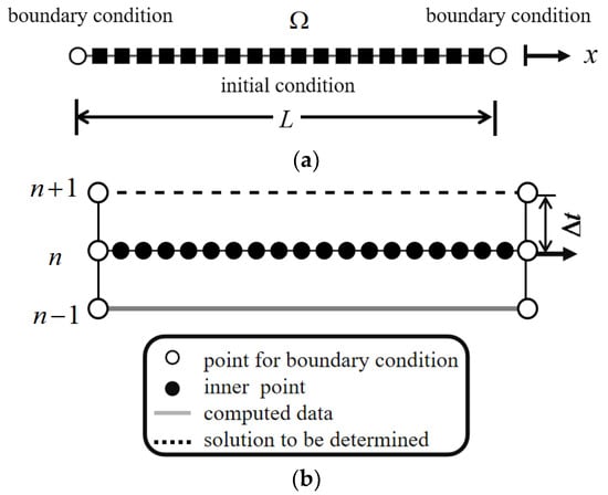
Figure 1.
Illustration of the one-dimensional time marching method. (a) Domain for discretization. (b) Time marching method.
Using the time-dependent PDE, the general temporal derivatives of the node at the time of the unknown nodes can be determined (the marching node graph of the scheme is shown in Figure 1b). Let and evaluate for and , for is a positive integer as follows:
where is the time step. In Equation (4), the forward Euler method is described at and in Equation (5), the backward Euler method is described at . As a combination of the forward and backward Euler methods, the Crank–Nicolson method can be described as follows:
The Crank–Nicolson method is based on the trapezoidal rule, which exhibits second-order convergence in time and is stable. Thus, in this study it is applied to the time marching process.
2.1.2. Space-Time Method
The ST method converts the original N-dimensional Euclidean space into an augmented (N + 1)-dimensional ST domain [10,21,24,25]. More specifically, time is treated as an augmented axis, and the number of spatial dimensions is greater than that of the original problem by one. The elapsed time is and the governing equation is expressed as Equation (1). Figure 2 illustrates the initial collocation points and the boundary collocation points in ST domain for a one-dimensional transient problem. In the ST domain, the boundary condition (i.e., Equation (2)), along with the augmented time axis at the collocation points are accessible, such that the initial condition (i.e., Equation (3)) is regarded as the boundary condition. The boundary and initial data are referred to as the ST boundary conditions.
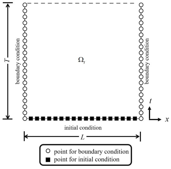
Figure 2.
Illustration of one-dimensional ST method.
2.1.3. Space-Time Marching Method
The majority of physical problems have unpredictable reaction times. To overcome this limitation, the ST marching method is employed in the numerical scheme. Note that conventional ST marching schemes lead to error accumulation. In order to reduce the error accumulation, a novel ST marching scheme is proposed that improves the traditional scheme.
Figure 3 shows the numerical process by which the ST domain is subdivided into ST subdomains. The length of time in each ST subdomain is . Two ST subdomains are adopted in the simulation area, and the numerical procedure follows the ST method. The numerical solution at the final time of the two ST subdomains in the computational domain is used as the initial condition of the next stage. All remaining ST subdomains are calculated using this method. By employing this method to determine the initial condition, the traditional time-marching errors can be reduced.
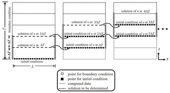
Figure 3.
Illustration of the one-dimensional ST marching method.
2.2. Space-Time Polyharmonic Radial Polynomial Basis Functions
The one-dimensional transient flow governing equation in porous media is expressed as follows:
where represents the diffusion coefficient, is the convective velocity, is the reaction coefficient, and is a source/sink function. Equation (7) presents a governing equation that describes the reaction mechanisms, convection effects, diffusion, and source/sink transport interactions.
The solutions of the governing equations are numerically approximated as a linear combination of the RBF as follows:
where is the radial distance from the source point to an arbitrary point, and is expressed as , is the RBF, x denotes the interior points and is expressed as , denotes the source points and is expressed as , refers to the number of source points; refers to the unknown coefficient. Various RBFs can be implemented in the RBFCM, including multiquadrics (MQ), Gaussian, inverse multiquadrics (IMQ) [13], and polyharmonic spline (PS) RBFs [10,26]. However, the accuracy of MQ, IMQ, and Gaussian RBFs can vary depending on the shape parameter. Therefore, the majority of applications for these RBFs rely on optimization or experimental techniques to determine their optimal shape parameters [27]. The PSRBF can achieve good results without requiring extra parameters to prevent singularities. Based on this, a meshless approach is presented here to solve the partial differential equations using the ST polyharmonic RPBFs [10]. The proposed RPBFs with the natural logarithm are defined as follows:
where denotes the terms of the RPBFs. The derivative of Equation (9) with respect to is as follows:
The derivative of Equation (9) with respect to t is then taken to obtain the following:
while the derivative of Equation (10) with respect to x is taken to yield the following:
Based on the ST domain of the one-dimensional PDE depicted in Equation (7) and the proposed RPBFs, the following equations can be derived:
where refers to the unknown coefficient. This approach can be used to approximate the solution of the PDE, and the following linear equation system is obtained:
where is a matrix for the boundary points and has a size of ; is an matrix of the interior points; is the unknown coefficient vector with elements; represents an source/sink data vector, written as ; denotes an boundary data vector, written as ; and represent the number of boundary points and internal points, respectively. Equation (13) becomes singular for , and the interior and source points have the same position. In order to avoid this singularity, a fictitious source is adopted, which must be located outside the domain [10,13]. More specifically, the source points of the RBF are treated as fictitious sources and placed outside the domain (Figure 4). The parametric equations that define the irregular boundary of the exterior source collocation are described as follows:
where denotes the position of the fictitious sources at jth source point; denotes the angle of the fictitious sources at jth source point; denotes the radius of the fictitious sources at jth source point. While outside source collocation boundaries are irregular, and is defined as follows:
where and represent the dilation parameter. Based on Equation (16) and considering different dilation parameter values, the source point positions can be correlated. In order to avoid the radial distance equaling zero, the original piecewise smooth radial function is converted into infinitely smooth RPBFs with fictitious sources scattered outside the domain. This avoids the singularity of the conventional RPBFs. Thus, the terms in Equation (13) are always smooth, and no extra techniques are required to deal with the singularity.
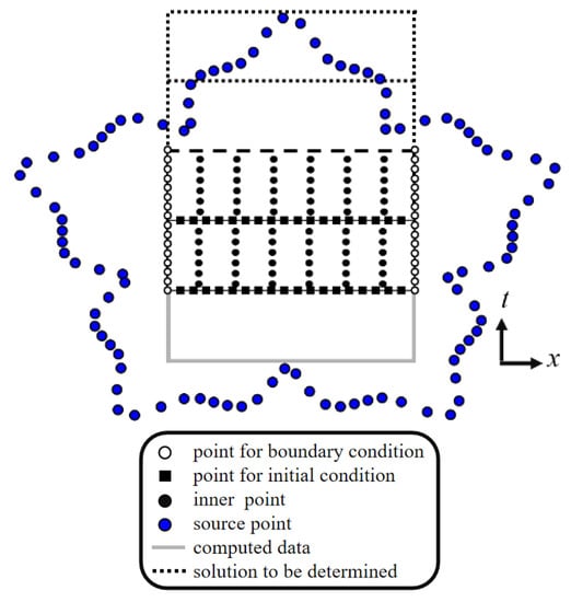
Figure 4.
Illustration of the collocation scheme for one-dimensional ST marching method.
2.3. Fictitious Time Integration Method
The governing equation expressed in Equation (7) is a nonlinear algebraic equation when and are functions of . The FTIM [28] based on a dynamical system is used to solve nonlinear equations and ignores the derivation of the Jacobian matrix. In this study, the FTIM is applied to solve the nonlinear algebraic system acquired using the ST polyharmonic RPBFs. By spatially and temporally discretizing the ST polyharmonic RPBFs, the FTIM is adopted for the system of nonlinear algebraic equations.
where are the interior points, is the radial distance from the source point to an interior point, are the boundary points, and is the radial distance from the center point to a boundary point. By solving Equations (17) and (18), the physical variable and the coefficient can be obtained. We adopted the FTIM to solve Equations (17) and (18) using the following iterative equations:
where m takes a value between zero and one; denotes the time step size; v indicates the non-zero coefficients; is the discrete time at p, such that ; and are the values of and at , respectively.
The iterative process begins with primary guess and ends when the stopping criteria are met, which can be described as follows:
where is the stopping criteria.
3. Validation
The numerical methods and results for the discretization of the transient flow equations are presented in this section. The number of validation points is , and the analytical and numerical solutions are evaluated at the ith validation point. The max absolute error (MAE) is defined as follows:
Additionally, the root mean square error (RMSE) is defined as follows:
We use three methods, namely, the time marching, ST, and ST marching methods, to calculate the one-dimensional transient problem and compare the corresponding accuracies. In this example, the space domain length (L) and elapsed time () are set to 0.5 and 60, respectively. The diffusion coefficient () is set at 0.05, and the convective velocity (), reaction coefficient (), and source/sink term are set at 0. The governing equation is as follows:
The boundary conditions on the right-and left-hand sides of the domain are expressed as follows:
The initial condition is defined as follows:
and the analytical solution is obtained as follows:
The PSRBF adopts a radial basis function of and the internal and source points are at the same location (Figure 5a). There are 99 interior points and two boundary points. For the temporal discretization of flow equations, we adopt the following Crank–Nicolson method:
with a time step of 1.5 × 10⁻².
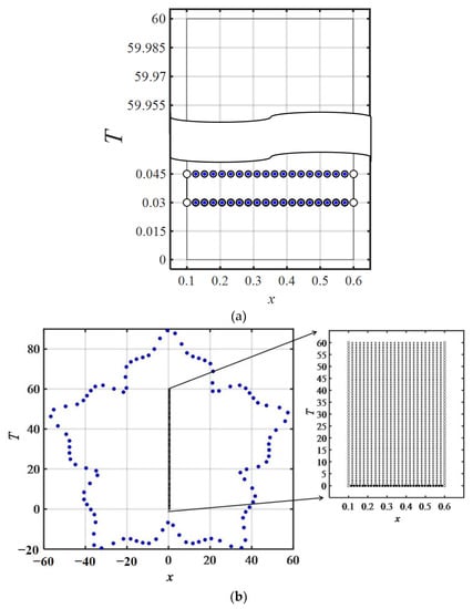
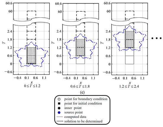
Figure 5.
Collocation scheme for: (a) time marching method; (b) ST method; (c) ST marching method.
The ST polyharmonic RPBFs have an initial value located at the bottom of the ST coordinate system, and the boundary values are shown on the left and right sides of Figure 5b. As demonstrated in Figure 5b, we collocated the interior, boundary, and fictitious sources within, on, and outside the ST domain, respectively. The numerical implementation consists of 900 interior points, 8101 boundary points, and 100 source points, with the dilation parameters and equal to 4 and 12, respectively, and the RPBF term () set as 11.
For the ST polyharmonic RPBFs combined with the ST marching method, the initial conditions for the computation domain of two ST subdomains are only known for the previous ST subdomain at the beginning of the simulations. There are 900 interior points, 100 fictitious sources, and 200 boundary points. Following the first calculation process, the number of interior points, fictitious sources, and boundary points are 900, 100, and 320, respectively. We collocated the interior, boundary, and external sources (Figure 5c). The RPBF term () equals 11, and the dilation parameters and are set as 4 and 1, respectively. In order to evaluate the accuracy and stability of the proposed method, we compare the results of the proposed method with the time marching and ST methods.
Figure 6 plots the MAE versus the simulation time of the three methods. With the implementation of the PSRBF and ST RPBF, the MAE can reach the order of 10−3 (Figure 6a,b). For the proposed ST marching method, the MAE reaches the order of 10−6 within the time range of 0–60 (Figure 6c) and reduces the error accumulation from the time marching approach. The results reveal the high accuracy and stability of the proposed ST marching method.
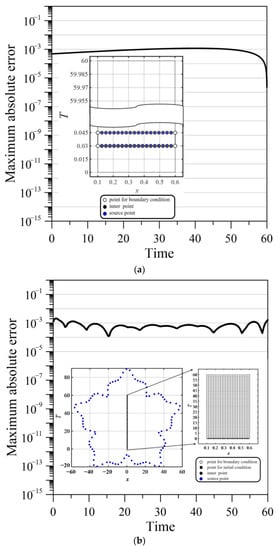
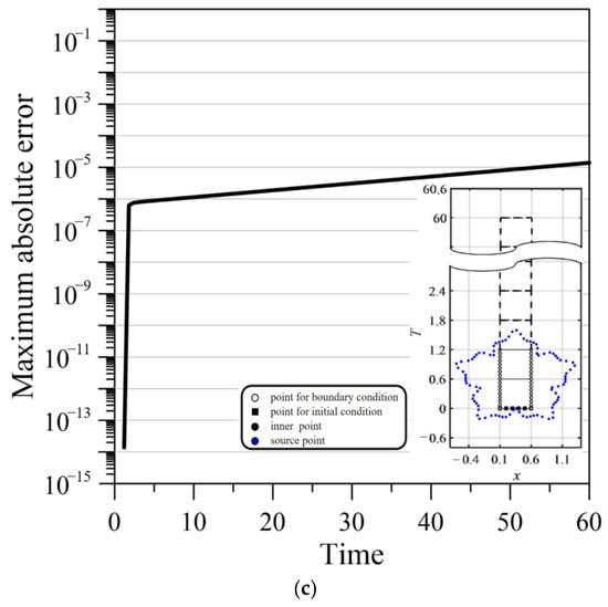
Figure 6.
Error comparison of three methods. (a) MAE versus simulation time for time marching method. (b) MAE versus simulation time for ST method. (c) MAE versus simulation time for ST marching method.
4. Numerical Example
4.1. Diffusion Equation with Sources and Sinks
In porous media, the governing equation, namely, the diffusion with sources and sinks, can be expressed as in Equation (7). The convective velocity () and reaction coefficient () are set to zero, the diffusion coefficient () along the x-axis is 1, and the source/sink term is then defined accordingly:
The Dirichlet boundary conditions are as follows:
The initial condition is as follows:
Additionally, the analytical solution is described as follows:
In this example, for the RPBF term () equal to 8, the expansion coefficients and are 4 and 1, and represents the duration of each computational ST domain. At the beginning of the simulation, there are 480 boundary points, 900 internal points, and 172 source points. As the time axis moves forward, there will be 640 boundary points, 900 internal points, and 172 source points in each computational ST domain. Figure 7 depicts the RMSE for the proposed method, respectively. As the time increases, the RMSE remains below . Table 1 compares the computational RMSE of the proposed approach with that of the meshless local radial point interpolation (MLRPI) and FDM with different ∆x and ∆t, where ∆x is the distance between the nodes in the x direction [14]. MLRPI and FDM have RMSE values of 10−5 and 10−4, respectively, while that of the proposed approach is 10−9.
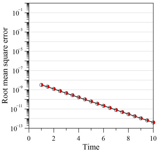
Figure 7.
Plot of RMSE versus simulation time.

Table 1.
RMSE values for the numerical example of the diffusion equation with sources/sinks.
4.2. Convection–Diffusion Equation
Next, we investigate the numerical solution of the convection-diffusion equation. As shown in Equation (7), this problem is governed by this equation. In the considered problem, the reaction coefficient () and source/sink terms are set to zero. defines the size of the geometry. The Dirichlet boundary conditions are applied as follows:
The initial condition is described as follows:
and the analytical solution is expressed as follows:
The convection–diffusion equation is used to represent substance diffusion and concentration change. The diffusion coefficient is fixed at 0.1 and the convection velocity is determined as follows:
For the study area, , the computation is performed for the RPBF term () equal to 8, expansion coefficients and , and represents the duration of each computational ST domain. At the beginning of the simulation, there are 480 boundary points, 900 internal points, and 172 source points. As the time axis moves forward, in each computational ST domain, the number of boundary points, internal points, and source points are 640, 900, and 172, respectively. The RMSE of the Lattice Boltzmann method can reach an order of 10−3 [29]. According to Figure 8, the proposed method has an RMSE of 10−6. The results prove that the proposed approach is more accurate than the Boltzmann method, indicating that it is better suited for high-accuracy applications.
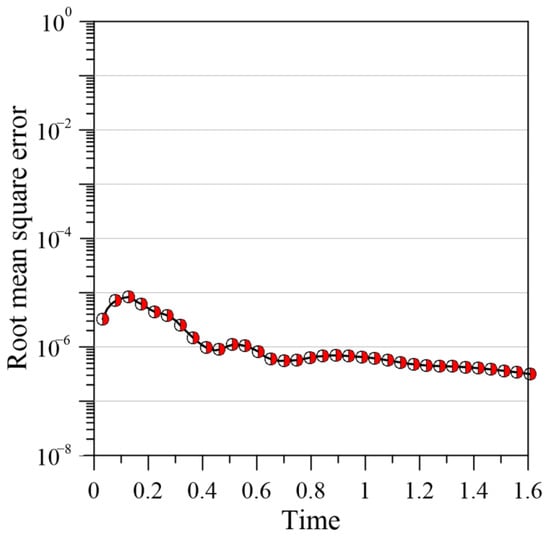
Figure 8.
RMSE versus simulation time.
4.3. Burgers–Fisher Equation
The Burgers–Fisher equation plays a key role in fluid dynamics models. Numerous authors have examined this model to conceptually understand physical flows and to test different numerical approaches. As a combination of convection, diffusion, and reaction mechanisms, the Burgers–Fisher equation is highly nonlinear. It is known as Burgers–Fisher as it inherits convective phenomena properties from the Burgers equation and diffusion transport properties from the Fisher equation. The Burgers–Fisher equation is given by the following:
According to Equation (37), the parameter values considered are as follows: , , . As a result, the governing equation can be written as follows:
where the final time is 1. For this problem, the Dirichlet conditions are described as follows:
The initial condition is the following:
and the analytical solution is obtained as follows:
In this example, the RPBF term () is equal to 6, and the expansion coefficients , and are 4.5 and 1, respectively, and for each computational ST domain. At the beginning of the simulation, there are 180 boundary points, 900 internal points, and 120 source points. With time, each computational ST domain will have 260 boundary points, 900 internal points, and 120 source points. The parameters , , , and are considered in this numerical implementation. Numerical simulations are used to compare the experimental results with the semi-implicit method and modified Crank–Nicolson method [16]. According to Figure 9, the MAE of the proposed method can reach an order of 10−9, while the semi-implicit method and modified Crank–Nicolson method with are able to achieve MAEs of 10−9 and 10−8, respectively. Thus, the ST marching method provides a greater accuracy with fewer data points, as demonstrated by this example.
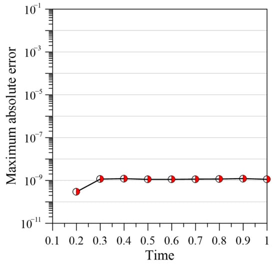
Figure 9.
MAE versus simulation time.
5. Conclusions
In this study, we present the novel ST marching method combined with the ST RBFCM and the FTIM to solve nonlinear transient flow problems in porous media. In particular, the ST RBFCM technique based on the collation of polynomial basis functions was applied. The proposed method does not require neither mesh nor numerical integration, but only collocation points on the computational domain, which is advantageous when the domain shape is irregular. Accordingly, the proposed method is advantageous for dealing with linear and nonlinear transient problems.
In contrast to the conventional time marching method, the proposed method can overcome limitations such as error accumulation in long periods for the conventional time marching method. Furthermore, the dense and ill-conditioned matrices created by the excessive number of boundary points and interior points, and the large ST radial distances can be avoided. The proposed method not only produces highly accurate results but also successfully minimizes the error accumulation compared to the conventional time marching method.
In order to solve the nonlinear problems, we proposed the novel ST marching numerical schemes combined with the FTIM. Three numerical examples, including the diffusion equation with sources and sinks, the convection-diffusion equation, and the Burgers–Fisher equation, were successfully solved using the proposed method. The numerical results were compared with the analytical solution, revealing a strong agreement between these two. Results demonstrate that the proposed method achieves a high accuracy in solving linear and nonlinear transient problems. Compared to the conventional time marching method and ST method, the proposed meshless approach provides more accurate solutions and reduces error accumulation. Since the current study considers only one-dimensional transient problems, future work is suggested to apply the proposed method to high-dimensional problems.
Author Contributions
Conceptualization, L.-D.H. and C.-Y.K.; methodology, C.-Y.K. and L.-D.H.; validation, L.-D.H.; data curation, L.-D.H. and C.-Y.L.; writing—original draft preparation, L.-D.H.; writing—review and editing, L.-D.H., C.-Y.K. and C.-Y.L.; visualization, L.-D.H. All authors have read and agreed to the published version of the manuscript.
Funding
This research received no external funding.
Institutional Review Board Statement
Not applicable.
Informed Consent Statement
Not applicable.
Data Availability Statement
The datasets generated during the study are available on request.
Acknowledgments
The authors are grateful to the anonymous referee involved for providing his/her invaluable comments and advice in this manuscript.
Conflicts of Interest
The authors declare that there is no conflict of interest.
Abbreviations
| PDEs | partial differential equations |
| FDM | finite difference method |
| RBFCM | radial basis function collocation method |
| ST | space-time |
| FTIM | fictitious time integration method |
| MQ | multiquadrics |
| IMQ | inverse multiquadrics |
| PS | polyharmonic spline |
| RPBFs | radial polynomial basis functions |
| MAE | max absolute error |
| RMSE | root mean square error |
| MLRPI | meshless local radial point interpolation |
References
- Tartakovsky, D.M.; Dentz, M. Diffusion in porous media: Phenomena and mechanisms. Transp. Porous Media 2019, 130, 105–127. [Google Scholar] [CrossRef]
- Carstea, A.S. Reaction-diffusion-convection equations in two spatial dimensions; continuous and discrete dynamics. Mod. Phys. Lett. B 2021, 35, 2150186. [Google Scholar] [CrossRef]
- Parhizi, M.; Kilaz, G.; Ostanek, J.K.; Jain, A. Analytical solution of the convection-diffusion-reaction-source (CDRS) equation using Green’s function technique. Int. Commun. Heat Mass Transf. 2022, 131, 105869. [Google Scholar] [CrossRef]
- Plawsky, J.L. Transport Phenomena Fundamentals, 2nd ed.; CRC Press: Boca Raton, FL, USA, 2009; pp. 31–69. [Google Scholar] [CrossRef]
- John, V.; Schmeyer, E. Finite element methods for time-dependent convection-diffusion-reaction equations with small diffusion. Comput. Methods Appl. Mech. Eng. 2008, 198, 475–494. [Google Scholar] [CrossRef]
- Mickens, R.; Gumel, A. Construction and analysis of a non-standard finite difference scheme for the Burgers-Fisher equation. J. Sound Vib. 2002, 257, 791–797. [Google Scholar] [CrossRef]
- Qu, W.; Gu, Y.; Zhang, Y.; Fan, C.M.; Zhang, C. A combined scheme of generalized finite difference method and Krylov deferred correction technique for highly accurate solution of transient heat conduction problems. Int. J. Numer. Methods Eng. 2019, 117, 63–83. [Google Scholar] [CrossRef]
- Gu, Y.; Qu, W.; Chen, W.; Song, L.; Zhang, C. The generalized finite difference method for long-time dynamic modeling of three-dimensional coupled thermoelasticity problems. J. Comput. Phys. 2019, 384, 42–59. [Google Scholar] [CrossRef]
- Ku, C.Y.; Hong, L.D.; Liu, C.Y.; Xiao, J.E.; Huang, W.P. Modeling transient flows in heterogeneous layered porous media using the space-time Trefftz method. Appl. Sci. 2021, 11, 3421. [Google Scholar] [CrossRef]
- Ku, C.Y.; Hong, L.D.; Liu, C.Y.; Xiao, J.E. Space-time polyharmonic radial polynomial basis functions for modeling saturated and unsaturated flows. Eng. Comput. 2021, 38, 4947–4960. [Google Scholar] [CrossRef]
- Grabski, J.K.; Kołodziej, J.A. Laminar fluid flow and heat transfer in an internally corrugated tube by means of the method of fundamental solutions and radial basis functions. Comput. Math. Appl. 2018, 75, 1413–1433. [Google Scholar] [CrossRef]
- Lin, J.; Bai, J.; Reutskiy, S.; Lu, J. A novel RBF-based meshless method for solving time-fractional transport equations in 2D and 3D arbitrary domains. Eng. Comput. 2022, 1–18. [Google Scholar] [CrossRef]
- Liu, C.Y.; Ku, C.Y. A simplified radial basis function method with exterior fictitious sources for elliptic boundary value problems. Mathematics 2022, 10, 1622. [Google Scholar] [CrossRef]
- Shivanian, E.; Khodabandehlo, H.R. Application of meshless local radial point interpolation (MLRPI) on a one-dimensional inverse heat conduction problem. Ain Shams Eng. J. 2016, 7, 993–1000. [Google Scholar] [CrossRef]
- Su, L. A radial basis function (RBF)-finite difference (FD) method for the backward heat conduction problem. Appl. Math. Comput. 2019, 354, 232–247. [Google Scholar] [CrossRef]
- Chandraker, V.; Awasthi, A.; Jayaraj, S. Numerical treatment of Burger-Fisher equation. Procedia Technol. 2016, 25, 1217–1225. [Google Scholar] [CrossRef]
- Amiri-Hezaveh, A.; Masud, A.; Ostoja-Starzewsk, M. Convolution finite element method: An alternative approach for time integration and time-marching algorithms. Comput. Mech. 2021, 68, 667–696. [Google Scholar] [CrossRef]
- Wang, H.; Zhang, Q. The direct discontinuous galerkin methods with Implicit-Explicit Runge-Kutta time marching for linear Convection-Diffusion problems. Commun. Appl. Math. Comput. 2022, 4, 271–292. [Google Scholar] [CrossRef]
- Ngondiep, E. Unconditional stability over long time intervals of a two-level coupled MacCormack/Crank-Nicolson method for evolutionary mixed Stokes-Darcy model. J. Comput. Appl. Math. 2022, 409, 114148. [Google Scholar] [CrossRef]
- Qi, L.; Hou, Y. An unconditionally energy-stable linear Crank-Nicolson scheme for the Swift-Hohenberg equation. Appl. Numer. Math. 2022, 181, 46–58. [Google Scholar] [CrossRef]
- Ku, C.Y.; Hong, L.D.; Liu, C.Y. Solving transient groundwater inverse problems using space–time collocation Trefftz method. Water 2020, 12, 3580. [Google Scholar] [CrossRef]
- Li, P.W.; Grabski, J.K.; Fan, C.M.; Wang, F. A space-time generalized finite difference method for solving unsteady double-diffusive natural convection in fluid-saturated porous media. Eng. Anal. Bound. Elem. 2022, 142, 138–152. [Google Scholar] [CrossRef]
- Fang, J.; Nadeem, M.; Habib, M.; Akgül, A. Numerical Investigation of Nonlinear Shock Wave Equations with Fractional Order in Propagating Disturbance. Symmetry 2022, 14, 1179. [Google Scholar] [CrossRef]
- Li, Z.; Mao, X.Z. Global space-time multiquadric method for inverse heat conduction problem. Int. J. Numer. Methods Eng. 2011, 3, 355–379. [Google Scholar] [CrossRef]
- Grabski, J.K. On the sources placement in the method of fundamental solutions for time-dependent heat conduction problems. Comput. Math. Appl. 2021, 88, 33–51. [Google Scholar] [CrossRef]
- Tsai, C.C.; Quadir, M.E.; Hwung, H.H.; Hsu, T.W. Particular solution of polyharmonic spline associated with reissner plate problems. J. Mech. 2011, 27, 493–501. [Google Scholar] [CrossRef]
- Saffah, Z.; Timesli, A.; Lahmam, H.; Azouani, A.; Amdi, M. New collocation path-following approach for the optimal shape parameter using Kernel method. SN Appl. Sci. 2021, 3, 249. [Google Scholar] [CrossRef]
- Liu, C.S.; Atluri, S.N. A novel time integration method for solving a large system of non-linear algebraic equations. Comput. Model. Eng. Sci. 2008, 31, 71–83. [Google Scholar] [CrossRef]
- Chai, Z.; Zhao, T. Lattice Boltzmann model for the convection-diffusion equation. Phys. Rev. E 2013, 87, 063309. [Google Scholar] [CrossRef]


Publisher’s Note: MDPI stays neutral with regard to jurisdictional claims in published maps and institutional affiliations. |
© 2022 by the authors. Licensee MDPI, Basel, Switzerland. This article is an open access article distributed under the terms and conditions of the Creative Commons Attribution (CC BY) license (https://creativecommons.org/licenses/by/4.0/).