
Componentwise Perturbation Analysis of the QR Decomposition of a Matrix

Department of Engineering Sciences, Bulgarian Academy of Sciences, 1040 Sofia, Bulgaria
Mathematics 2022, 10(24), 4687; https://doi.org/10.3390/math10244687
Submission received: 17 November 2022
/
Revised: 4 December 2022
/
Accepted: 6 December 2022
/
Published: 10 December 2022
(This article belongs to the Special Issue Numerical Analysis and Matrix Computations: Theory and Applications)
Abstract
:The paper presents a rigorous perturbation analysis of the QR decomposition of an matrix A using the method of splitting operators. New asymptotic componentwise perturbation bounds are derived for the elements of Q and R and the subspaces spanned by the first columns of A. The new bounds are less conservative than the known bounds and are significantly better than the normwise bounds. An iterative scheme is proposed to determine global componentwise bounds in the case of perturbations for which such bounds are valid. Several numerical results are given that illustrate the analysis and the quality of the bounds obtained.
Keywords:
QR decomposition; perturbation analysis; componentwise bounds; asymptotic bounds; global boundsMSC:
65F25; 47A55; 93C731. Introduction
The QR decomposition of a matrix with as the factorization
where is an orthogonal matrix and is the upper triangular matrix. The matrices Q and R are referred to as the Q-factor and the R-factor, respectively. Further on, we shall assume that the matrix A has rank m, i.e., it has full column rank. In such a case, the matrix R is nonsingular, and the matrix Q can be represented as
where and the columns of form an orthonormal basis for the complementary subspace ([1], Ch. 1). Thus,
The representation (2) is frequently called QR factorization of A, and it is unique up to the signs of the diagonal elements of R. The matrix is not unique but has to obey the orthogonality condition
In practice, the matrix A is subject to perturbations of different kinds (model inconsistencies, measurement and rounding errors), which leads to the necessity of investigating the sensitivity of the different elements of the QR decomposition to perturbations in the data, i.e., to perform a perturbation analysis of the decomposition [2]. Further on, we assume that the matrix A is subject to an additive perturbation and that there exist another pair of matrix and upper triangular matrix such that
The purpose of the perturbation analysis of the QR decomposition is to find bounds on the sizes of and as functions of the size of for sufficiently small perturbations of A [3,4]. Due to the non-uniqueness of the matrix , its perturbation is also non-unique. Thus, in the perturbation analysis, one usually considers only the perturbations of the matrix , which are uniquely defined by the perturbations of A. However, in the analysis, we shall need to use an arbitrary matrix that satisfies the orthogonality condition (3).
The sizes of the perturbations , and in the QR factorization are measured by using some of the matrix norms, and, in this case, we call the respective analysis normwise perturbation analysis. Sometimes, however, we are interested in the size of perturbations in individual elements of and , and, in such a case, the analysis is called componentwise perturbation analysis [5]. In the cases when the estimated vector or matrix has components that differ greatly in size, the normwise estimate does not produce reliable results, and it is preferable to use the componentwise perturbation analysis.
The perturbation analysis of the QR decomposition was performed for the first time by Stewart [6], and improved results were presented by Sun [7] and Stewart [8]. Using a different approach, Chang, Paige and Stewart [9] gave new asymptotic perturbation bounds for the R-factor. Additional improvements of the normwise perturbation bounds of the QR-decomposition were proposed by Chang and Stehlé [10] and Li and Wei [11]. Different componentwise estimates of the perturbations of the Q-factor and the R-factor were derived by Sun [12], Zha [13], Chang and Paige [14] and Chang [15].
A general approach, based on the use of the so-called splitting operators, which can be used in the perturbation analysis of several unitary decompositions, was proposed in [16]; for details, see [17]. The method of the splitting operators can be used to determine normwise as well as componentwise perturbation bounds of different unitary decompositions; see [18,19,20,21,22]. This method was implemented by Sun [23], who obtained improved normwise perturbation bounds of the QR decomposition.
This paper presents a rigorous componentwise perturbation analysis of the QR decomposition based on the method of splitting operators. The analysis presented aims at finding normwise and componentwise perturbation bounds for infinitely small perturbations (asymptotic bounds) as well as for finite perturbations (global bounds). The main result is the obtaining of new asymptotic componentwise perturbation bounds that produce less conservative estimates of the QR decomposition perturbations. A particular case of these bounds is the asymptotic normwise bounds of the QR decomposition derived previously.
This is demonstrated by an example that the new componentwise perturbation bounds of the R factor can be several orders of magnitude smaller than the normwise perturbation bound of this factor. An iterative scheme is proposed to determine global componentwise bounds in the case of perturbations for which such bounds exist. The analysis conducted in this paper is unified with the perturbation analysis of the Schur decomposition presented in [20] and can be easily extended to the case of complex matrices.
In Section 2, we introduce the basic scheme of the perturbation analysis. Section 3 is devoted to determining normwise and componentwise perturbation bounds of the matrix . In Section 4, we present estimates for the perturbations of the column subspaces of A, and, in Section 5, we derive bounds of the elements of R. An iterative scheme for finding global componentwise perturbation bounds of the QR decomposition is proposed in Section 6. A comparison with some of the known methods for perturbation analysis of the QR decomposition is performed in Section 7, and our conclusions are made in Section 8.
The numerical results presented in the paper were obtained with MATLAB® R2020b [24] using IEEE double precision arithmetic with roundoff unit .
2. Bounding the Basic Perturbation Parameters
Let
and the unperturbed and perturbed matrices of the orthogonal factor of the QR decomposition be
respectively. Define the perturbation matrix
The column can be obtained from the QR factorization (2) as
Since , it follows that
and
These quantities, which we call basic perturbation parameters, are elements of the strict lower part of the matrix . More precisely, one has that
or, equivalently,
where
Define the lower triangular matrix
whose elements are determined entirely from the elements of R. It can be shown that
The matrix M has the form
which shows that this matrix is nonsingular if the diagonal elements of R are nonzero. The matrix M is called the perturbation operator matrix.
From (9), we obtain that
where
and the vector has components
containing second-order terms in the perturbations .
The norm of this approximation obeys
which shows that the size of the linear bound of depends on . As shown by Sun [23],
Since
one obtains the asymptotic normwise bound
Since the matrix M is lower triangular, it is usually inverted with high precision. Using (12), one can obtain asymptotic componentwise bounds on the perturbation vector x. Since
it follows that
and using the inequality , one obtains the asymptotic bound
The quantity can be considered as a componentwise condition number [25] of the element .
Example 1.
Consider the matrix
and assume that it is perturbed by
where c and k are varying parameters. The QR decompositions of matrices A and are computed by the function qr of MATLAB®. In the given case, the perturbation operator matrix M is of order and .
The exact absolute values of the elements of the vector x and their linear approximations computed according to (12) for three perturbations , and of different size, are given to five decimal digits in the third and fourth columns of Table 1, respectively. It is seen that the elements of the linear estimate closely follow the corresponding elements of the exact perturbation vector .
3. Bounding the Perturbations of the Matrix
Consider the matrix
The strictly lower part of this matrix contains elements of the form
which can be substituted by the corresponding elements of the vector x. The elements of the strictly upper part of are of the form
which, according to the orthogonality condition (8), can be represented as
In this way, the matrix can be written as
where the matrix
has elements depending only on the basic perturbation parameters,
and the matrix
contains second-order terms in .
Consider how to determine the diagonal elements of the matrix W (the nontrivial elements of D) from the elements of x. Denote that . According to (8), one has that
or
The above expression shows that is always nonnegative.
On the other hand, we have that
so that
From
it follows that
The negative solution of this equation is
For a small perturbation (small values of ), one has the estimate
Thus, for small perturbations, the quantities depend quadratically on .
In Table 2, for the same matrix and perturbations that are given in Example 1, we give the exact values of and their linear and nonlinear estimates computed using the exact vectors x.
Thus, having the linear approximations of the elements of x, one can compute the linear approximations of the matrices and . According to (16), the sum is the linear approximation of , and contains second-order terms in that can be neglected in the asymptotic analysis. As shown below, the determining of an estimate of allows one to find a bound on .
3.1. Normwise Bounds
The estimate of can be used to find an asymptotic normwise bound of . In determining condition numbers, one assumes , so that . From Equation (16), it follows that the Frobenius norm of the strictly upper triangular part of the matrix is less than (if ) or equal (if ) to the norm of the strictly lower part . Since , we have that , and the change of the matrix obeys
where is an asymptotic normwise bound on and
can be considered as a normwise condition number of the matrix with respect to the perturbations of A.
Since, in first-order approximation, it is fulfilled that
considering (21), one obtains that
where
is the normwise condition number of the matrix R with respect to the perturbation .
3.2. Componentwise Bounds
The componentwise bounds of the elements of the matrix can be found by using the componentwise estimates of the elements of x. An asymptotic bound on the matrix is given by
Considering that and using (16), a linear approximation of the perturbation is determined as
This equation gives asymptotic bounds of the perturbations in the individual elements , i.e., componentwise perturbation bounds of the matrix . Since = , we have that
i.e., the obtaining of the asymptotic componentwise estimate through (23) may increase the bounds on at most times.
In Table 3, we give, for the same QR decomposition as the one presented in Example 1, the exact values of and their linear approximations for . The comparison of the componentwise bounds with the normwise linear bound shows that the bounds on the individual elements of are smaller than for all . The difference between the componentwise and normwise bounds is particularly significant for the elements in the first column of whose absolute values are of order , while the normwise bound is of order .
4. Estimating Column Subspace Sensitivity
The determination of bounds on the elements of the matrix makes it possible to estimate the sensitivity of the column subspaces . (Note that, for , the corresponding column subspace coincides with the range of A.) Since we assume that R is of full rank, we have that , i.e., the first columns of Q form an orthonormal basis for the subspace .
As is known [26], the sensitivity of a subspace of dimension p is measured by the p angles between the perturbed and unperturbed subspace. Let and be the orthonormal bases for and its perturbed counterpart , respectively. Then, the maximum angle between and is determined from [26]
where is the orthogonal complement of , . Since
one has that
Equation (25) shows that the sensitivity of the column subspace is related to the values of the basic perturbation parameters . In particular, for , the sensitivity of the first column of A is determined as
for , one has
and so on (see Figure 1).
In this way, if the basic perturbation parameters are known, it is possible to find the sensitivity estimates of all column subspaces with dimension . More specifically, let
Then, we have that the maximum angle between the perturbed and unperturbed column subspace of dimension p is
In particular, for the sensitivity of , we obtain that
An asymptotic estimate of the maximum angle can be obtained, if, in the expression for the matrix , the elements are replaced by their linear approximations (12). Representing the matrix as
the matrix can be written as
where the rows of are highlighted in boxes,
and
Using the fact that
we obtain the following asymptotic estimate,
Thus, an asymptotic bound of is determined as
where the quantity
can be considered as a condition number of the column subspace . The derivation of is performed such that to find its possible minimum value.
In Table 4, we give the exact values of maximum angle and its asymptotic bound for the perturbation problem considered in Example 1. In all cases, the size of the estimate matches correctly the size of the actual maximum angle between the perturbed and unperturbed subspace.
5. Perturbation Bounds of the Elements of R
It is convenient to first consider the sensitivity of the nontrivial elements of the upper triangular matrix R for the case of the diagonal elements. Due to the nonsingularity of R, these elements are nonzero.
5.1. Sensitivity Estimates of the Diagonal Elements of R
The changes in the elements of the perturbed matrix R satisfy
The above equation can be rewritten as
Using Equations (7) and (8), one obtains for the perturbations of the diagonal () elements of R, the expressions
Further on, we shall use the following quantities:
- The diagonal elements of the matrix ,
- The changes of the diagonal elements of R,
- The diagonal elements of W,
Denote the columns of as and the columns of as . Then, the system of Equation (30) can be represented as
where
and the matrix was defined earlier. Neglecting the quadratic terms in (31), one obtains the linear estimate
Equation (32) can be represented in the compact form
Since
it follows from (33) that the asymptotic perturbation satisfies
where
is considered as a condition number of . The derivation of (35) is performed to find the minimum possible value of .
In Table 5, for the matrix A and the perturbations given in Example 1, we present the exact perturbations of the diagonal elements of R and their linear and nonlinear estimates. The normwise quantities and are the normwise linear and nonlinear bounds, derived in [17,23]. These bounds are more pessimistic than the bounds and .
5.2. Sensitivity Estimates of the Super Diagonal Elements of R
According to (29), the perturbations of the super diagonal elements of the matrix R can be determined as
Let us define the vectors (the elements of the corresponding matrices are taken row-wise),
and
where
Then, Equation (36) may be represented as the system of nonlinear algebraic equations
where and are matrices whose elements are functions of the elements of R. These matrices are determined from
where
and is the vec-permutation matrix as determined from ([27], Ch. 4)
In a linear approximation, one has
and it is possible to show that
where
Neglecting the second-order terms in Equation (38) and using the linear estimate , one obtains the asymptotic estimate
Let us denote
Since
one concludes that, in a first-order approximation, the super diagonal elements of fulfill
where
Equation (40) gives asymptotic componentwise perturbation bounds for the super diagonal part of R. The quantity represents the condition number of with respect to the perturbations in A.
In Table 6, for the matrix A and the perturbations given in Example 1, we give the exact perturbations of the super diagonal elements of R and their linear estimates. As in the case of the diagonal elements, the normwise linear and nonlinear bounds and give worse estimates than .
6. Determining Global Perturbation Bounds
Based on the analysis presented above, it is possible to derive an iterative scheme for finding global perturbation bounds of the QR decomposition. The main task of such a scheme is to find a nonlinear estimate of the vector x of the basic perturbation parameters. For this aim, it is necessary to estimate the quadratic term in (10). The analysis of the expression (10) shows that contains terms involving the perturbations for , which are not estimates up to the moment since they are columns of the matrix . As mentioned previously, the matrix is not unique, and consequently its perturbation is also non-unique. However, the problem with finding of the minimum norm for a fixed has a unique solution, and our first task in this section is to find an approximation of this perturbation.
6.1. Perturbation Bounds of the Columns of
Setting , we obtain that
where . (Note that is already estimated). For sufficiently small perturbations , the matrix is nonsingular, and we have that
In the first-order analysis of (47), the term can be neglected, and we have the approximation
The expression (49) shows that the size of the minimum norm matrix is of second order regarding to the size of , and hence can be neglected in the asymptotic analysis of (46). Thus, we obtain the first-order approximations
In this way, the matrix
is approximated as
and an approximation of is obtained as
In Table 7, for the perturbation problem presented in Example 1, we show the quantities related to the approximation of and the norms of the matrices
characterizing the errors in the orthogonal matrices and , respectively. The approximation of the perturbed orthogonal factor is obtained as
where is the exact perturbation of . These quantities are computed for the three perturbations and . The results given in the table confirm the assumptions from the perturbation analysis of .
For the same example used previously, in Table 8, we give the exact values of the elements of and their approximations using (52). The exact minimum norm perturbation is found numerically by solving the minimization problem
under the constraint . The minimization is performed by the MATLAB® function fmincon. The results show that, in all cases, is close to .
6.2. Iterative Procedure for Finding Global Bounds of the Elements of x
Since one has linear estimates of the basic perturbation terms , it is appropriate to substitute the terms containing the perturbations in Equation (16) by the perturbations
which are of the same size as . Since
the absolute value of the matrix (16) can be bounded as
where
Since the unknown column estimates participate in both sides of (53), it is possible to obtain recursively as follows.
Let
where and are the first columns of and , respectively. Then, the next column estimates can be determined as
where
If , the matrix is strictly diagonally dominant and nonsingular ([28], p. 352) and if are small, then the condition number of is close to 1.
The matrix only gives estimates of the first m columns of . Using the representation
one can find an approximation of the matrix using the Equations (50) and (51). Thus, an approximation of is obtained as
After determining estimates of , it is possible to bound the absolute values of the quadratic terms , given in (11), as
The column represents an estimate of such that .
In this way, one obtains an iterative scheme involving Equations (11) and (53)–(55). At each step s, the value of the nonlinear estimate of x is determined from
with initial condition , where is the MATLAB® function eps, . The stopping criterion is taken as
This scheme converges for perturbations of restricted size. As shown in ([17], Ch. 4), the size of the maximum allowable perturbation for which the nonlinear normwise estimate of x is valid is given by
where .
In Table 9, we present the number of iterations necessary to find the nonlinear estimate for the perturbation problem considered in Example 1, along with and . The components of are shown for three different perturbations in the fifth column of Table 1 along with the vectors and .
In Figure 2, we show the convergence of the relative error as a function of s for different perturbations . As is seen from the figure, with the increasing perturbation size, the convergence worsens, and, for , the iterations do not converge since the global bound does not exist. The convergence of the iterations is linear, and this can be improved by using appropriate optimization techniques.
6.3. Global Perturbation Bounds of , Column Subspaces and R
Implementing the obtained nonlinear estimate of x, one may find nonlocal bounds on the perturbations of the column subspaces, diagonal and super diagonal elements of R using Equations (26), (31) and (38).
After determining the nonlinear bounds of x and , it is possible to find nonlinear bounds on the perturbations of the elements of according to the relationship
The nonlinear bounds of the elements of for the QR decomposition given in Example 1 and a perturbation are shown in the last column of Table 3 along with and .
A global estimate of the maximum angle between the perturbed and unperturbed column subspace of dimension p is obtained from (26). The values of for the matrix A from Example 1 and three different perturbations are given in the last rows of Table 4.
Nonlinear bounds on the diagonal elements of R can be obtained by using the expressions
and global bounds of the perturbations of the super diagonal elements of R can be found from
The nonlinear perturbation bounds of the diagonal elements of R for the matrix A from Example 1 and for three perturbations are given in Table 5, and the nonlinear bounds of the super diagonal elements are presented in Table 6. We note that the global perturbation estimates are slightly larger than the corresponding asymptotic estimates but give guaranteed bounds on the perturbations whenever these estimate exist.
7. Comparison with Other Bounds
In this section, we consider two examples in which we compare the perturbation bounds of the QR decomposition obtained in this paper with the bounds that were previously proposed.
Example 2.
Consider the fifth-order matrix [12],
The matrix A is nonsingular, and its QR factors are and . The perturbation matrix is the random matrix
Using the function qr of MATLAB®, we obtain (to four decimal digits) that
The nonlinear bound of the perturbation of Q, obtained after 16 iterations, is
The maximum element of the global estimate of , obtained in [12], is , while the maximum element of is . Furthermore, , while .
Example 3.
Consider a matrix A, taken as
where is an upper triangular matrix with unit diagonal and super diagonal elements equal to 3, and the matrix is constructed as proposed in [29],
where and are elementary reflections that are orthogonal and symmetric matrices [30]. The condition number of with respect to the inversion is controlled by the variable σ and is equal to . In the given case, σ is taken equal to , and . The minimum singular value of the matrix M satisfies
which means that the perturbations of Q and R can be several orders of magnitude larger than the perturbations of A. The perturbation of A is chosen as , where c is a positive number and is a matrix with random entries generated by the MATLAB® function rand.
Several results related to the perturbation problem under consideration for 30 values of c between 13 and 5 are given in Figure 3, Figure 4, Figure 5, Figure 6, Figure 7 and Figure 8. In Figure 3, we display the perturbations of the particular entry , which is an element of the matrix . The quantities and are the normwise linear and nonlinear bounds derived in [17,23].
These bounds are more than 12-times larger than the norms of the linear and nonlinear componentwise bounds obtained in Section 3. The nonlinear bound is close to the linear one for perturbations of different sizes and increases gradually in the vicinity of the quantity . For perturbations of a larger size, the iterations for do not converge. In Figure 4, we compare the exact perturbation of the entry (which is also the element of ) with the linear approximation . Both quantities are close for all perturbations. This is confirmed by the values of the errors
shown in Figure 5, which are much smaller than the value of for all perturbations.
The bounds of the quantity (the maximum angle between the perturbed and unperturbed range of A), shown in Figure 6, are close to the exact value of this angle, with the nonlinear bound being slightly greater than the linear one. The normwise linear and the nonlinear bounds obtained in [17,23], are more than 75,000-times greater than the linear and the nonlinear bounds of the diagonal element , shown in Figure 7. Similarly, the normwise bounds and are more than 13,000-times greater than the bounds and as shown in Figure 8. This large difference between the sizes of the actual component perturbations of R and the normwise bounds is explained by the large condition number of the computed R—equal to . (Note that ).
Note that, while the normwise estimates are valid for perturbations with sizes up to , the iterations to find converge for perturbations .
The results obtained show that the asymptotic bounds are valid for much larger perturbations then the global bounds.
8. Conclusions
The method presented in the paper allows us to find, in a unified manner, componentwise asymptotic and global perturbation bounds for all elements of the QR decomposition, thus, providing a complete perturbation analysis of this important matrix factorization. The bounds obtained in the paper are smaller than some known bounds and can be significantly better than the normwise bounds.
Funding
This research received no external funding.
Institutional Review Board Statement
Not applicable.
Informed Consent Statement
Not applicable.
Data Availability Statement
The datasets generated during the current study are available from the author on reasonable request.
Acknowledgments
The author is grateful to the reviewers for their remarks and suggestions that helped to improve the paper.
Conflicts of Interest
The author declares no conflict of interest.
Abbreviations
| the set of real numbers; | |
| the space of real matrices (); | |
| the range of A; | |
| the orthogonal complement of the subspace ; | |
| the matrix of absolute values of the elements of A; | |
| the transposed of A; | |
| the inverse of A; | |
| the pseudoinverse of A; | |
| the jth column of A; | |
| the ith row of matrix A; | |
| the part of matrix A from row to and from column to ; | |
| perturbation of A; | |
| the zero matrix; | |
| the unit matrix; | |
| the jth column of ; | |
| the minimum singular value of A; , equal by definition; | |
| ⪯ | relation of partial order. If , then means ; |
| the strictly lower triangular part of A; | |
| the strictly upper triangular part of A; | |
| the spectral norm of A; | |
| the Frobenius norm of A; | |
| the Kronecker product of A and B; | |
| the vec mapping of . If A is partitioned columnwise as | |
| then ; | |
| the vec-permutation matrix. ; | |
| the maximum angle between subspaces and ; | |
| a quantity of second order with respect to . |
Appendix A
Theorem A1.
The minimum Frobenius norm solution of the matrix equation
is given by
Proof.
Equation (A1) is represented as
where is the vec-permutation matrix satisfying . This matrix is symmetric and orthogonal and has eigenvalues equal to 1 and eigenvalues equal to −1 ([27], p. 265). Hence, for some orthogonal U, it may be represented as
so that
The minimum 2-norm solution of (A3), corresponding to the minimum Frobenius solution of (A1), is given by
where
Thus,
and
Since
it follows that
q.e.d. □
References
- Stewart, G.W. Matrix Algorithms; Vol. I: Basic Decompositions; SIAM: Philadelphia, PA, USA, 1998; ISBN 0-89871-414-1. [Google Scholar]
- Stewart, G.W.; Sun, J.-G. Matrix Perturbation Theory; Academic Press: San Diego, CA, USA, 1990; ISBN 978-0126702309. [Google Scholar]
- Bhatia, R. Matrix factorizations and their perturbations. Linear Algebra Appl. 1994, 197, 245–276. [Google Scholar] [CrossRef] [Green Version]
- Li, R. Matrix perturbation theory. In Handbook of Linear Algebra, 2nd ed.; Hogben, L., Ed.; CRC Press: Boca Raton, FL, USA, 2014; Chapter 21; pp. 1–20. [Google Scholar]
- Higham, N. A survey of componentwise perturbation theory in numerical linear algebra. In Mathematics of Computation 1943–1993: A Half Century of Computational Mathematics; Gautchi, W., Ed.; Amer. Mathematical Society: Providence, RI, USA, 1994; pp. 49–77. ISBN 0-8218-0291-7. [Google Scholar]
- Stewart, G.W. Perturbation bounds for the QR factorization of a matrix. SIAM J. Numer. Anal. 1977, 14, 509–518. [Google Scholar] [CrossRef]
- Sun, J.-G. Perturbation bounds for the Cholesky and QR factorizations. BIT Numer. Math. 1991, 31, 341–352. [Google Scholar] [CrossRef]
- Stewart, G.W. On the perturbation of LU, Cholesky, and QR factorizations. SIAM J. Matrix Anal. Appl. 1993, 14, 1141–1145. [Google Scholar] [CrossRef] [Green Version]
- Chang, X.-W.; Paige, C.C.; Stewart, G.W. Perturbation analyses for the QR factorization. SIAM J. Matrix Anal. Appl. 1997, 18, 1328–1340. [Google Scholar] [CrossRef] [Green Version]
- Chang, X.-W.; Stehlé, D. Rigorous perturbation bounds of some matrix factorizations. SIAM J. Matrix Anal. Appl. 2010, 31, 2841–2859. [Google Scholar] [CrossRef] [Green Version]
- Li, H.; Wei, Y. Improved rigorous perturbation bounds for the LU and QR factorizations. Numer. Linear Algebra Appl. 2015, 22, 1115–1130. [Google Scholar] [CrossRef]
- Sun, J.-G. Componentwise perturbation bounds for some matrix decompositions. BIT Numer. Math. 1992, 32, 702–714. [Google Scholar] [CrossRef]
- Zha, H.Y. A componentwise perturbation analysis of the QR decomposition. SIAM J. Matrix Anal. Appl. 1995, 14, 1124–1131. [Google Scholar] [CrossRef]
- Chang, X.-W.; Paige, C.C. Componentwise perturbation analyses for the QR factorization. Numer. Math. 2001, 88, 319–345. [Google Scholar] [CrossRef]
- Chang, X.-W. On the perturbation of the Q-factor of the QR factorization. Numer. Linear Algebra Appl. 2012, 19, 607–619. [Google Scholar] [CrossRef]
- Konstantinov, M.M.; Petkov, P.H.; Christov, N.D. Nonlocal perturbation analysis of the Schur system of a matrix. SIAM J. Matrix Anal. Appl. 1994, 15, 383–392. [Google Scholar] [CrossRef]
- Konstantinov, M.M.; Petkov, P.H. Perturbation Methods in Matrix Analysis and Control; NOVA Science Publishers, Inc.: New York, NY, USA, 2020; ISBN 978-1-53617-470-0. [Google Scholar]
- Chen, X.S. Perturbation bounds for the periodic Schur decomposition. BIT Numer. Math. 2010, 50, 41–58. [Google Scholar] [CrossRef]
- Chen, X.S.; Li, W.; Ng, M.K. Perturbation analysis for antitriangular Schur decomposition. SIAM J. Matrix Anal. Appl. 2012, 33, 1328–1340. [Google Scholar] [CrossRef]
- Petkov, P. Componentwise perturbation analysis of the Schur decomposition of a matrix. SIAM J. Matrix Anal. Appl. 2021, 42, 108–133. [Google Scholar] [CrossRef]
- Sun, J.-G. Perturbation bounds for the generalized Schur decomposition. SIAM J. Matrix Anal. Appl. 1995, 16, 1328–1340. [Google Scholar] [CrossRef]
- Zhang, G.; Li, H.; Wei, Y. Componentwise perturbation analysis for the generalized Schur decomposition. Calcolo 2022, 59. [Google Scholar] [CrossRef]
- Sun, J.-G. On perturbation bounds for the QR factorization. Linear Algebra Appl. 1995, 215, 95–112. [Google Scholar] [CrossRef] [Green Version]
- MATLAB Version 9.9.0.1538559 (R2020b) Update 3; The MathWorks, Inc.: Natick, MA, USA, 2020.
- Gohberg, I.; Koltracht, I. Mixed, componentwise, and structured condition numbers. SIAM J. Matrix Anal. Appl. 1993, 14, 688–704. [Google Scholar] [CrossRef]
- Björck, Å.; Golub, G. Numerical methods for computing angles between linear subspaces. Math. Comp. 1973, 27, 579–594. [Google Scholar] [CrossRef]
- Horn, R.A.; Johnson, C.R. Topics in Matrix Analysis; Cambridge University Press: Cambridge, UK, 1991; ISBN 0-521-30587-X. [Google Scholar]
- Horn, R.A.; Johnson, C.R. Matrix Analysis, 2nd ed.; Cambridge University Press: Cambridge, UK, 2013; ISBN 978-0-521-83940-2. [Google Scholar]
- Bavely, C.A.; Stewart, G.W. An algorithm for computing reducing subspaces by block diagonalization. SIAM J. Numer. Anal. 1979, 16, 359–367. [Google Scholar] [CrossRef]
- Stewart, G.W. Matrix Algorithms; Vol. II: Eigensystems; SIAM: Philadelphia, PA, USA, 2001; ISBN 0-89871-503-2. [Google Scholar]
Figure 1.
Perturbation estimates of the column subspaces.
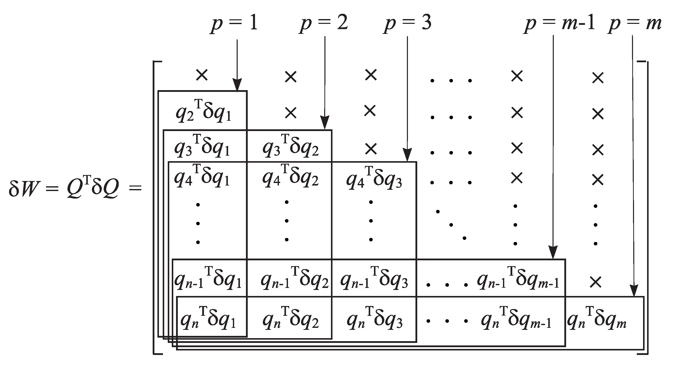
Figure 2.
Iterations for determining the global bounds for different perturbations.

Figure 3.
Exact values of and its bounds as functions of the perturbation norm.

Figure 4.
Exact values of and its bounds as functions of the perturbation norm.

Figure 5.
The errors as functions of the perturbation norm.

Figure 6.
Exact values of and its bounds as functions of the perturbation norm.

Figure 7.
Exact values of and its bounds as functions of the perturbation norm.

Figure 8.
Exact values of and its bounds as functions of the perturbation norm.


Table 1.
Exact basic perturbation parameters and their linear and nonlinear estimates.
| 1 | 2 | 3 | 4 | 5 |
Table 2.
Approximation of the diagonal elements of matrix W.
Table 3.
Exact perturbations of the elements of the matrix and their linear and nonlinear estimates, , , and .
Table 3.
Exact perturbations of the elements of the matrix and their linear and nonlinear estimates, , , and .
Table 4.
Exact perturbations of the maximum subspace angles and their linear and nonlinear estimates.
Table 4.
Exact perturbations of the maximum subspace angles and their linear and nonlinear estimates.
Table 5.
Exact perturbations of the diagonal elements of R and their linear and nonlinear bounds.
Table 6.
Exact perturbations of the super diagonal elements of R and their linear and nonlinear bounds.
Table 6.
Exact perturbations of the super diagonal elements of R and their linear and nonlinear bounds.
Table 7.
Quantities related to the approximation of .
| , | , | ||
| , | , | ||
| , | |||
Table 8.
Approximated perturbations of the elements of and their approximations.
Table 9.
Convergence of the global bounds.
| k | Number of Iterations | |||
|---|---|---|---|---|
| 4 | ||||
| 4 | ||||
| 5 | ||||
| 6 | ||||
| 9 | ||||
| 17 | ||||
| No convergence | - |
Publisher’s Note: MDPI stays neutral with regard to jurisdictional claims in published maps and institutional affiliations. |
© 2022 by the author. Licensee MDPI, Basel, Switzerland. This article is an open access article distributed under the terms and conditions of the Creative Commons Attribution (CC BY) license (https://creativecommons.org/licenses/by/4.0/).
Share and Cite
MDPI and ACS Style
Petkov, P.H. Componentwise Perturbation Analysis of the QR Decomposition of a Matrix. Mathematics 2022, 10, 4687. https://doi.org/10.3390/math10244687
AMA Style
Petkov PH. Componentwise Perturbation Analysis of the QR Decomposition of a Matrix. Mathematics. 2022; 10(24):4687. https://doi.org/10.3390/math10244687
Chicago/Turabian StylePetkov, Petko H. 2022. "Componentwise Perturbation Analysis of the QR Decomposition of a Matrix" Mathematics 10, no. 24: 4687. https://doi.org/10.3390/math10244687
Note that from the first issue of 2016, this journal uses article numbers instead of page numbers. See further details here.