4.1. Soft Sensing Modeling of Cell Voltage Based on STA-LSSVM
When the evaluation results of the cell state are excellent and good, energy consumption can be reduced by lowering the cell voltage. In the current electrolytic cell industry, lowering the cell voltage means reducing the pole distance. However, simply reducing the pole distance will definitely affect the current efficiency and stability of the aluminum electrolytic cell and ultimately reduce aluminum production. Therefore, in order to reduce the cell voltage without decreasing the current efficiency, the parameters that affect the cell voltage can only be adjusted within a reasonable range.
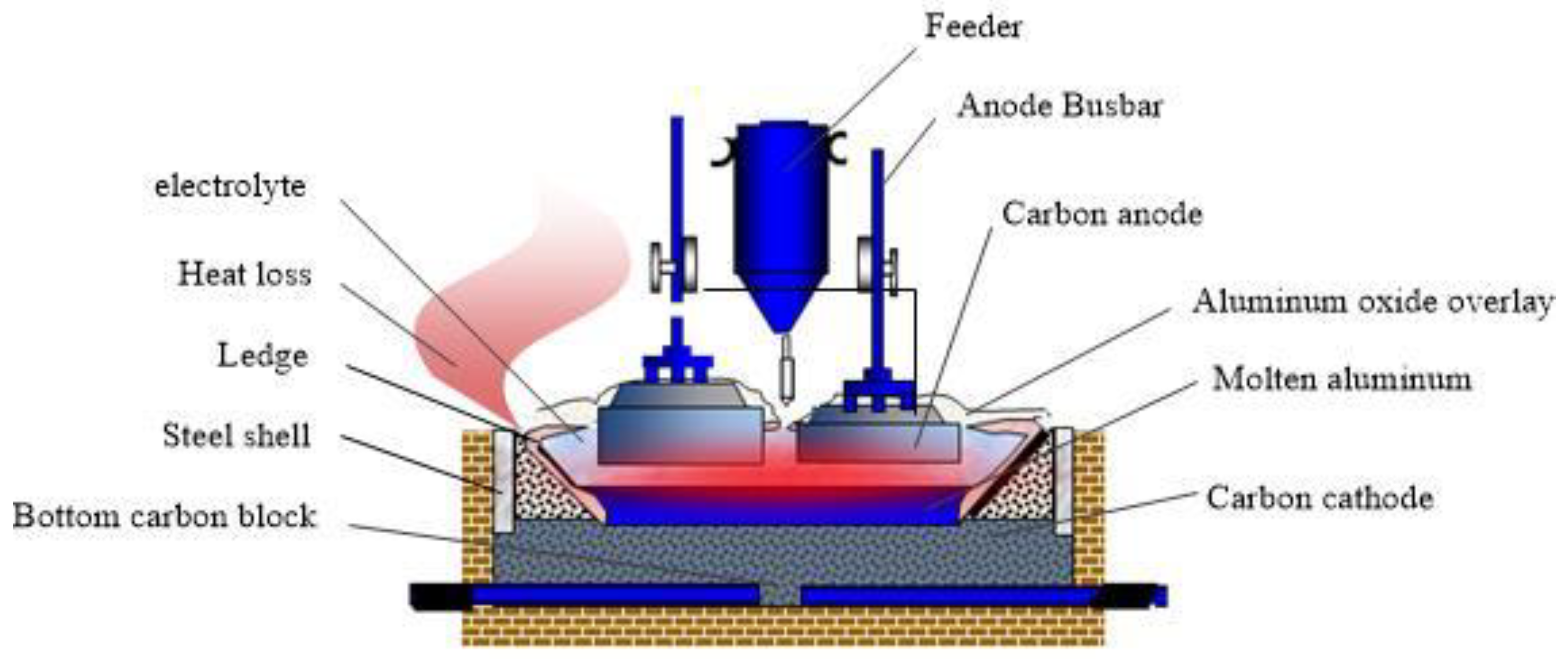
There are many cell voltage parameters that affect the change of aluminum electrolysis. Cell resistance and current intensity directly reflect the change in cell voltage. Alumina concentration, electrolyte temperature, and molecular ratio have significant effects on the change of electrolyte conductivity, thus affecting the stability of cell voltage. Moreover, an important reason for the anode effect is that the cell voltage rises rapidly when the alumina concentration is low, which destroys the balance state of the electrolytic cell; The electrode distance is the distance from the anode bottom to the cathode aluminum liquid mirror. It has a direct impact on cell resistance, resulting in cell voltage change. The temperature of the electrolyte is affected by the height of the aluminum liquid. The height of aluminum liquid changes the thermal balance of the electrolytic cell and then changes the voltage stability of the cell; less anode wetted area causes the anode effect, so the electrolyte level needs to be maintained in a reasonable range to prevent the anode effect from affecting the voltage. When the aluminum level is too high, the heat dissipation in the cell increases, causing the cell bottom to become cold, affecting the thermal balance of the cell and thus affecting the cell voltage stability. Based on the above analysis, the parameters that affect the cell voltage are the pole distance (), electrolyte level (), cell resistance (), alumina concentration (), aluminum level (), current intensity (), and molecular ratio ().
In this paper, we use the least squares support vector machine to build a cell voltage prediction model. The LSSVM algorithm has a strong classification capability and requires less training time to train non-linear data with a large time delay and strong coupling. Based on the previous research, we found that the STA is better and more effective in reducing energy consumption by comparing the average value of the cell voltage optimized by ALO and STA [
38], so we decided to optimize the LSSVM prediction model by STA. The specific aluminum electrolyzer voltage prediction schematic is shown in
Figure 2.
STA treats a solution to the optimization problem as a state and finds the optimal solution by iterating and updating the state, which is regarded as a state transition process. The STA framework is shown as follows:
where
is a current state, it represents a candidate solution of the current optimization scheme,
or
is a state transition matrix with randomness and an operator of the basic state transition algorithm,
is a function of
containing historical state;
is the objective function or evaluation function;
is the fitness function value at point
.
The state transfer-based optimization-seeking algorithm uses four state transformation operators [
39], including rotation transformation, translation transformation, expansion transformation, and axial transformation, to solve a continuous optimization problem through evolution.
- (1)
(rotation transformation, RT):
- (2)
(translation transformation, TT):
- (3)
(expansion transformation, ET):
- (4)
(axesion transformation, AT):
where
,
are the rotation factor,
is the translation factor,
and
are the stretch factor and coordinate factor, respectively. They are all positive numbers greater than zero.
is a random matrix whose elements obey a uniform distribution of [−1,1],
is a Euclidean or 2-parametric number;
is a random variable whose elements obey a uniform distribution between
. The translation transformation is an algorithm for a line search, mainly along the vector direction from
to point
and with
as the starting point for a line search of maximum length
.
is a random diagonal array whose internal elements follow a standard normal distribution.
represents a random diagonal sparse matrix with non-zero elements only at one position and the elements absolutely obeying the standard normal distribution. Finally, for the properties of these four operators: the rotation transform is able to control the accuracy of the solution and accomplish the performance of the local search. It guarantees the optimal solution within a hypersphere of maximum radius
. The translation transform not only balances the local search and the global search but also refines the one-dimensional search. The stretching transformation is theoretically able to stretch each element in
to the range of
, allowing a global search to be completed.
The parameters of LSSVM should be chosen reasonably for the reasons that these parameters uniquely define a specific model and, at the same time, determine the model’s precision that greatly affects the accuracy and effectiveness of cell voltage optimization. In this paper, with RBF is chosen as the kernel function of LSSVM, there are only two parameters that need to be determined, the kernel function’s parameter and punishment factor . The STA algorithm is used to find the optimal parameters for better learning performance of LSSVM.
The realization steps of the STA-LSSVM algorithm are as follows:
Step 1: The input training set is divided into a training set and a test set.
Step 2: The parameters of the LSSVM model, the parameter of the Gaussian radial basis kernel function, and the punishment factor , are used as the two merit-seeking parameters to be identified for each set of the state transfer algorithm.
Step 3: Set STA parameters, such as iteration number and search enforcement (SE), Rotation factor , translation factor , expansion factor and coordinate factor .
Step 4: Generate the initial solution. Each solution of STA represents the combination option of two parameters that determine the LSSVM performance.
Step 5: During each iteration, the STA uses four operational operators in turn to generate candidate solutions, and the solution with a better fitness value for the training set is reserved for the next iteration.
Step 6: If the termination condition is met, the algorithm optimization process stops, and the LSSVM model training is completed. If the termination condition is not met, return to Step 5.
Step 7: In the test dataset, the STA-LSSVM model was used to predict the cell voltage and output the prediction results.
The flow chart of STA-LSSVM to build a cell voltage prediction model implementation is shown in
Figure 3.
4.2. Cell Voltage Optimization Model Based on STA
After the LSSVM prediction model is established, to realize the optimal control of the cell voltage and achieve the purpose of consumption reduction, it is necessary to find the optimal cell voltage and its corresponding optimal technical conditions under normal operating conditions.
Under normal operating conditions, the adjustment of the pole distance is an important tool for regulating the energy balance of the cell. The variation in the length of the pole distance directly affects the cell voltage. In various types of electrolytic cells, the pole distance is generally kept between 3.6~5 cm; a very important condition for the stable and efficient operation of electrolytic cells in aluminum production is to maintain a reasonable electrolyte level, which is between 14~23 cm. The alumina concentration represents the material balance in the cell and ranges from 1.9%~3.5%; in the production of aluminum electrolysis, the aluminum level can significantly affect the current efficiency. The molecular ratio is used to measure the acidity and alkalinity of the electrolyte and is traditionally characterized by the molecular ratio of NaF to AlF3. The molecular ratio should be maintained in the range of 2.1~2.7 and should not be at a lower level. In summary, the seven variables for the mechanistic analysis are set as pole distance (), electrolyte level (), cell resistance (), alumina concentration (), aluminum level (), current intensity (), molecular ratio (), and the optimal control model for cell voltage is established as shown in Equation (23).
Based on the above analysis, the mathematical description of the optimization model can be stated as follows:
The objective of Formula (15) is to find the lowest value of cell voltage under the seven constraints obtained from process analysis and gray correlation analysis, which can be regarded as a multi-objective optimization problem with multiple constraints. In this paper, STA is used to optimize the cell voltage optimization control model. Its optimization steps are:
Step 1: Random initialisation. Set the basic parameters of the algorithm and randomly generate SE = 50 states within a set range, each state representing a set of 7 × 1 cell voltage parameters.
Step 2: Using the cell state parameters in each initial state as input to the cell voltage prediction model, the fitness function value for each initial state is obtained, and the state with the lowest fitness value is taken as the current optimal set parameter value, with the corresponding fitness value taken as the optimal cell voltage.
Step 3: The iteration starts. The state is transformed according to the four optimization operators of the STA, and the value of the fitness function is calculated for the transformed state. The current state is changed only when the optimal value is obtained, updating the cell voltage value and the optimal setting parameters; otherwise, the optimal state is maintained.
Step 4: Determine if the difference between the adaptation value is less than the set threshold or if the maximum number of iterations is 1000, the algorithm ends if one of these criteria is met and the cell voltage optimization value is obtained; otherwise, go to Step 3.
The flowchart of optimization based on STA cell voltage is shown in
Figure 4.


