Abstract
Cross-domain fault diagnosis methods have been successfully and widely developed in the past years, which focus on practical industrial scenarios with training and testing data from numerous machinery working regimes. Due to the remarkable effectiveness in such problems, deep learning-based domain adaptation approaches have been attracting increasing attention. However, the existing methods in the literature are generally lower compared to environmental noise and data availability, and it is difficult to achieve promising performance under harsh practical conditions. This paper proposes a new cross-domain fault diagnosis method with enhanced robustness. Noisy labels are introduced to significantly increase the generalization ability of the data-driven model. Promising diagnosis performance can be obtained with strong noise interference in testing, as well as in practical cases with low-quality data. Experiments on two rotating machinery datasets are carried out for validation. The results indicate that the proposed algorithm is well suited to be applied in real industrial environments to achieve promising performance with variations of working conditions.
1. Introduction
Being the most essential part of any rotating machinery, the rolling element bearing has a wide range of applications in the manufacturing industry. Unexpected failures of mechanical components can result in heavy operational losses and serious safety concerns. Rotating elements are usually at a higher risk of mechanical failure due to the fatigue stresses experienced during their operation. Efficient and accurate fault detection and diagnosis is of vital significance, which not only helps to enhance production but also ensures improvement in reliability and operational safety of a machine. Over these years, different signal processing techniques have been utilized for analyzing vibration signals from mechanical systems and components to monitor their health condition. These traditional techniques, however, require expert knowledge about failure mechanics.
In recent times, there have been successful implementations of machine learning and deep learning-based methods for machinery condition monitoring. In deep learning models that are purely data driven, different layers are stacked together to form a deep network architecture. A complex network and deeper network generally results in more efficient feature extraction compared to shallower networks, which makes deep learning a very useful tool in machine health monitoring and fault diagnosis purposes [1,2,3].
To develop a deep learning-based fault diagnosis model, data are collected from the labeled healthy condition of the system [4,5,6]. The labeled data are then exploited for training model and subsequently predict the underlying machine health condition of the unlabeled testing data. However, this process is normally performed under the assumption that the data are obtained from a single distribution. In practical scenarios, the systems are operated under variable operating conditions in terms of speed and load. Therefore, there exists a discrepancy between the distributions of the training and testing data provided by the model [7]. This issue undermines the generalization ability of the model to obtain accurate results over different distributions. This problem is referred to as the domain shift phenomenon.
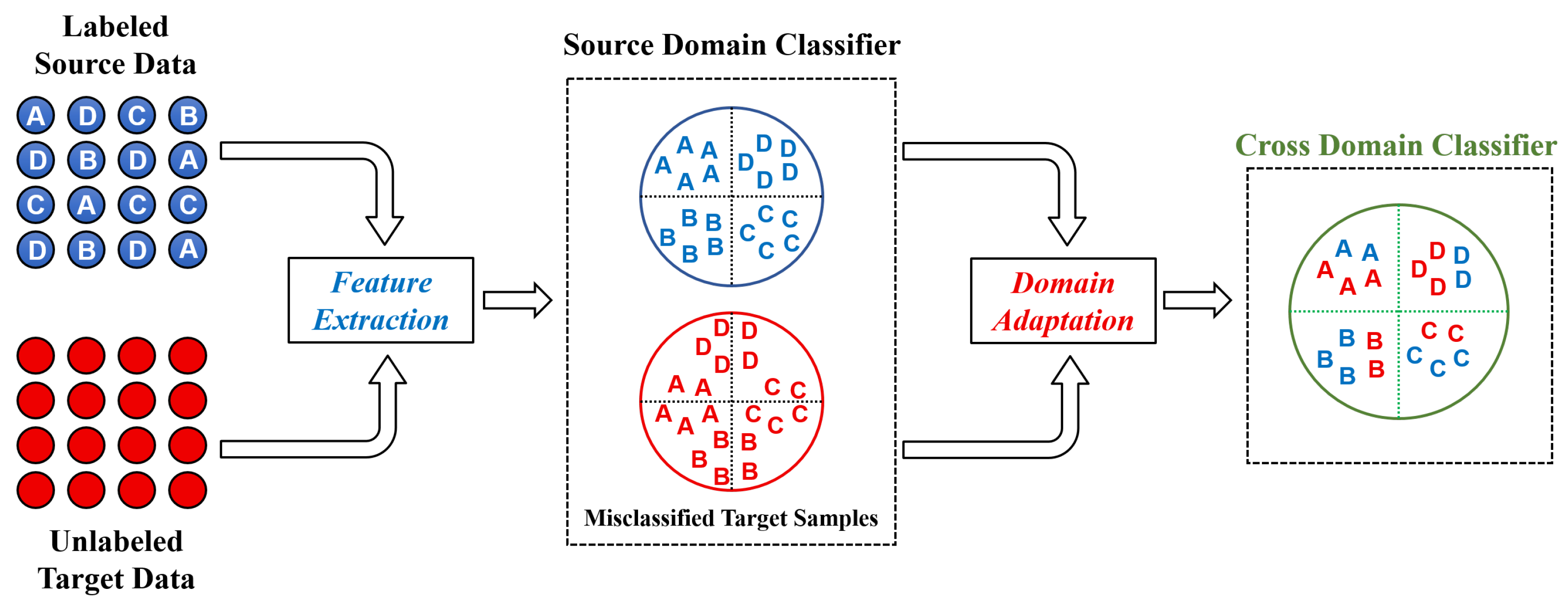
To address this issue, many deep learning-based approaches have been proposed to transfer the knowledge that is obtained from the source domain to the target domain while the target domain is collected under different operating conditions [8,9]. Hasan et al. [10] proposed a deep learning-based transfer learning approach to improve the feature extraction capability of bearing fault diagnosis systems. On the other hand, domain adaptation (DA) approaches are widely used to reduce the discrepancy between source and target domain data distributions [11,12,13,14]. As demonstrated in Figure 1, the distribution discrepancy between the source and target domains results in the ineffective performance of source domain classifier when applied in the target domain. Fundamentally, in most of DA approaches, the classifier built using source domain data is adapted for its use in the target domain by aligning the source and target domain distribution in a latent feature space.
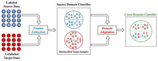
Figure 1.
The schematic representation of domain adaptation methodology.
In some situations, even with the application of cross-domain adaptation, there is still a significant distribution discrepancy between the source and target data that reduces the accuracy of the fault diagnosis models. Although data can be acquired easily using state-of-the-art sensors, it usually has a fixed representation and is mostly unlabeled. Moreover, most parts of the collected raw data comes from the healthy working condition of the machine with limited data from different faulty conditions [15]. This makes it difficult to develop a robust model that can be generalized over a wider range of machine health conditions. Li et al. [16] proposed a domain augmentation approach to improve the generalization of the deep learning-based fault diagnosis model. Hu et al. [17] suggests a data augmentation technique that uses a resampling technique to simulate data through partial overlap for different operating conditions. Gao et al. [18] used a Generative Adversarial Network (GAN) to artificially produce fake samples from the limited amount of training data for effective training of a robust cross domain classifier. Wang et al. [19] proposed a novel domain adaptation method based on adversarial networks for improving the waveform recognition performance in the target domain. In [20], the authors have exploited the idea of parameter freezing to ameliorate the performance in the target domain by freezing part of the model parameters and fine-tuning the rest for preventing overfitting issues.
To further enhance the effectiveness of the model, a novel algorithm is proposed in this paper for improving model performances in cross-domain adaptation scenarios. The key novelty and contributions of the paper is as follows:
- The health state labels in the form of one hot encoded vectors are induced with a random noise in the training stage.
- This increases the variability of the source dataset, making the training more robust and achieving better optimization of the model.
- This algorithm has been implemented on two different bearing datasets to validate the performance of the proposed approach.
2. Conceptual Background
2.1. Problem Formulation
A transfer learning problem for rotating machinery fault diagnosis is investigated in this paper. The knowledge is learned from the labeled source domain and unlabeled target domain samples using the distribution discrepancy metric. Let be the source domain, where shows the -dimensional source data, is the system health condition label and is the number of source samples. Likewise, the target domain is also denoted as , where represents the -dimensional target data, denotes the system health condition label and is the target sample. The source and target domain have identical label spaces in this study.
2.2. Convolutional Neural Networks
In this study, a convolutional neural network (CNN) architecture, including convolutional, pooling and fully connected (FC) layers, is utilized to establish a deep learning model for fault diagnosis purposes. The main function of a convolutional layer is to generate meaningful features by convolving raw input data with predefined filters. Subsequently, the most significant feature information is recognized by the pooling layer and is further propagated through the network. The convolution operation can be expressed as follows:
where and denote the j-th feature map at l-th layer. The convolutional kernel that connects the i-th feature map with j-th feature map of the l-th layer is denoted as . The term represents the bias, and operation ∗ is the convolution operation. The function is the activation function.
The length of the feature maps can be reduced within the pooling layers without losing key spatial information. Among the important operations, the max pooling operation extracts the maximum out of the set of values, predefined by the pooling size. After multiple alternating convolutional and pooling layers, abstract features are passed through the fully connected layer to perform the desired fault diagnosis task.
2.3. Maximum Mean Discrepancy
Maximum Mean Discrepancy (MMD) has been utilized as a discrepancy measurement between the considered distributions in this article [21]. For domain adaptation application, the MMD, as a non-parametric criterion, is used to compare the source and target distributions by measuring the squared distance between the kernel embeddings of marginal distributions mapped in the Reproducing Kernel Hilbert Space (RKHS). The following is the mathematical formulation:
where S and T are the data distribution corresponding to the source and target domains, respectively. The RKHS endowed with a characteristic kernel k is represented by . The operation is the mapping function, and denotes the expectation with regards to the distribution S.
As it is stated in [22], the process of calculating the MMD is highly influenced by the choice of kernels. Therefore, a combination of five radial basis function (RBF) kernels is used to exploit the power of multiple kernels (MK).
2.4. Concept of Noisy Health Labels
A novel technique is introduced in this study for enhancing the deep learning-based domain adaptation performance of the model in the fault diagnosis framework. For improving the model’s generalization ability, a random noise is injected into the health state labels of the data, for strong regularization purposes. With the help of this technique, data diversity can be elevated, and model randomness can be improved for better optimization.
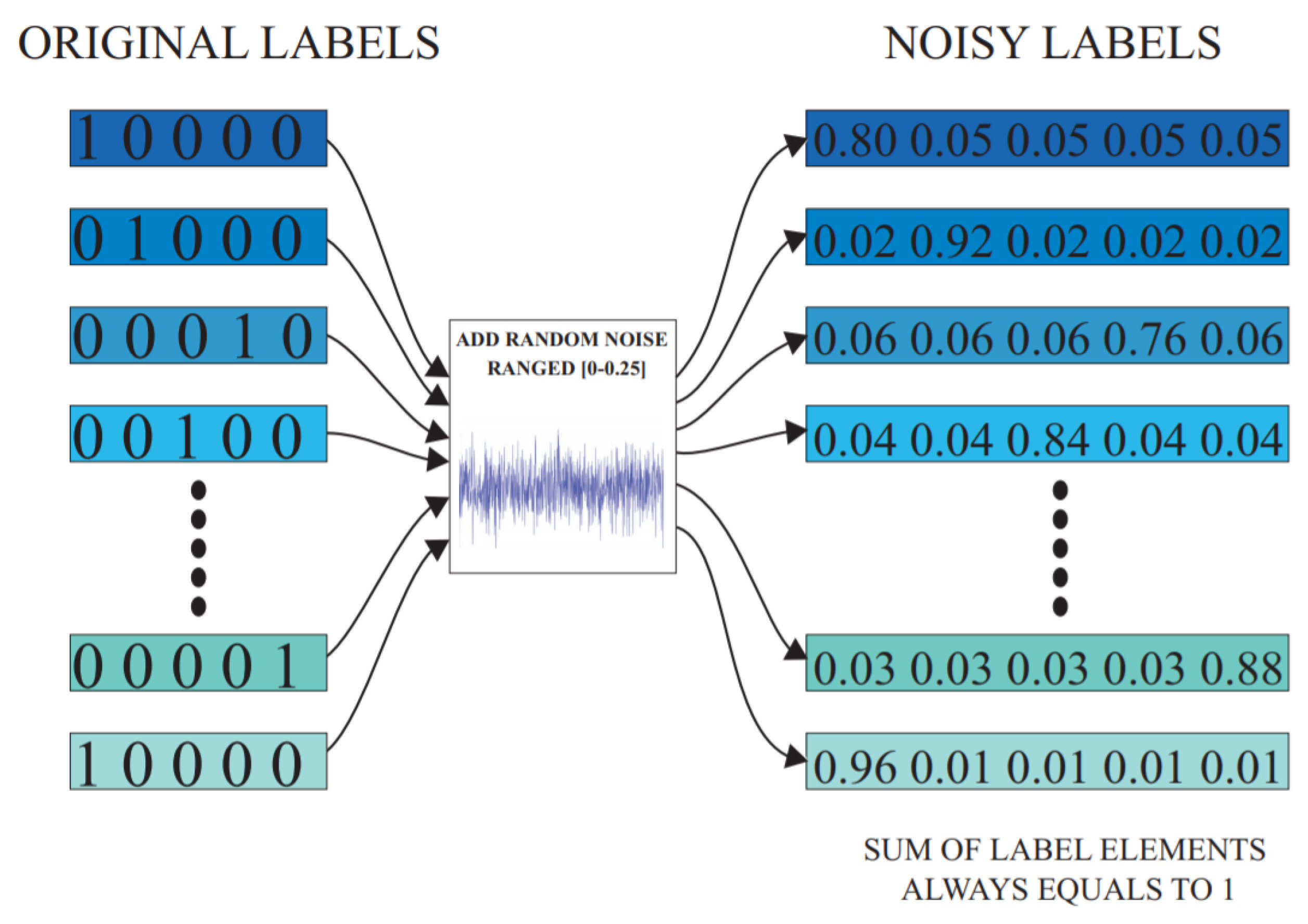
For the supervised classification tasks, the softmax layer in the deep learning model requires health condition labels in the form of one-hot encoded vectors. During the network’s training process, a random noise value is homogeneously selected from the interval , with reference to each labeled training data sample in the mini batch [23]. An optimal noise level is finalized for this study after running multiple experiments on the data. The results of these experiments are summarized in Section 4.3.2. The randomly selected noise value is then injected into the one-hot encoded health label of each training sample in the mini batch. As per the requirement of the softmax function, is subtracted from the true class element, and the corresponding increments are made in the remaining label elements to ensure the sum remains equal to unity.
For instance, consider as the one-hot encoded health label of a sample, where denotes the number of classes in the problem. After injecting a random noise value , the noisy health label thus becomes , . In this manner, the noisy health label still maintains its compatibility with the softmax function such as the typical one-hot vector labels. For a better understanding of this concept, a schematic representation of this proposed technique is presented in Figure 2.

Figure 2.
Illustrative explanation of the noisy label algorithm.
3. Proposed Method
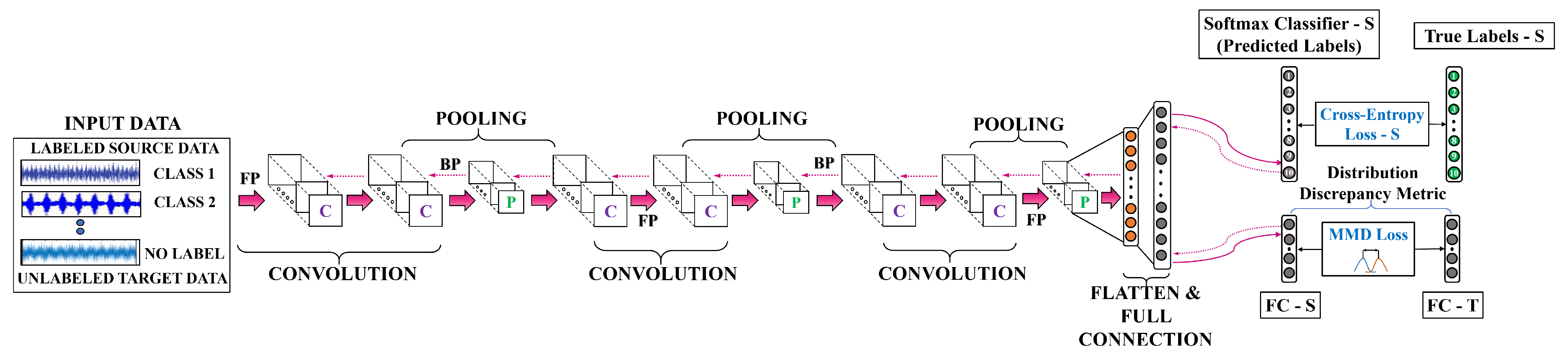
An illustrative explanation of the proposed CNN architecture has been presented in Figure 3. In this study, data are organized in two different groups, viz., source-domain data , and target-domain data . Raw vibration data have been directly used as input for the network. Without any specialized pre-processing, a windowing approach is used for preparing raw data samples for training. To extract high-level features from the raw data, three stacks of two consecutive 1D convolutional layers followed by a max-pooling operation have been designed. At the network’s final step, the learned features are used as the input of the fully connected layer for obtaining high-level representation. Commonly, the rectified linear units (ReLU) activation function is utilized all over the the network while the softmax activation function is exploited to obtain the desired classification output. The dropout technique has been employed to reduce the chance of overfitting phenomenon. Generally, the network optimization objective has two factors, which are detailed below.

Figure 3.
The proposed deep learning architecture for cross-domain fault diagnosis.
(1) Categorical cross-entropy loss: The suggested CNN architecture employs an objective function to reduce training sample classification errors. The usual cross-entropy loss function is used in this work, which is defined as follows:
where is the number of system health conditions, is the i-th sample’s predicted probability corresponding to the j-th class, while is the corresponding system condition label.
(2) Distribution discrepancy loss: The MMD metric is utilized in the optimization function to calculate and minimize the distribution discrepancy between source and target. The loss function can be formulated as follows:
where and denote high-level feature representations of the source and target domain in FC layer, respectively.
By integrating the two objective functions, the final objective function is derived as follows:
where and are the penalty coefficients for losses , and , respectively. The network’s parameters can be adjusted as follows during each training epoch:
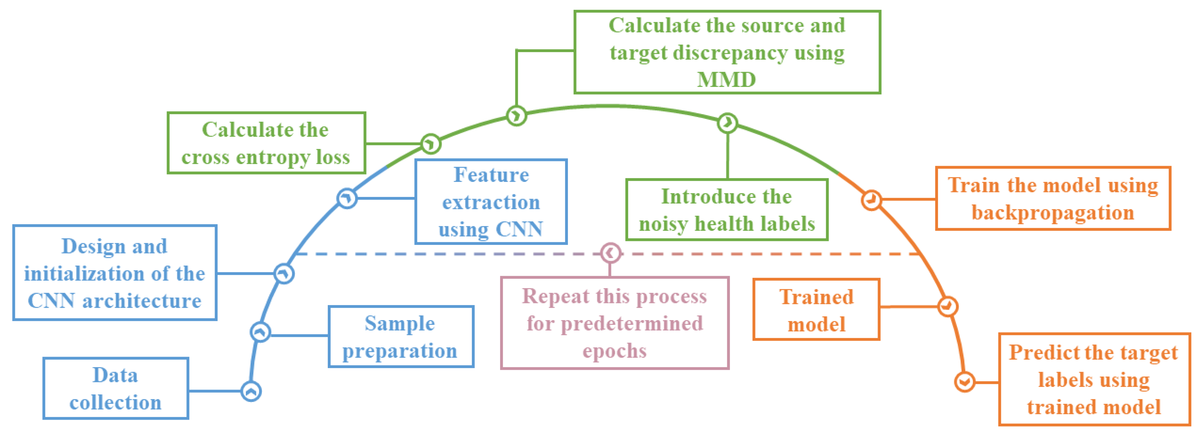
where and are the model parameters and learning rate, respectively. The flowchart of the proposed cross-domain fault diagnosis method is demonstrated in Figure 4.
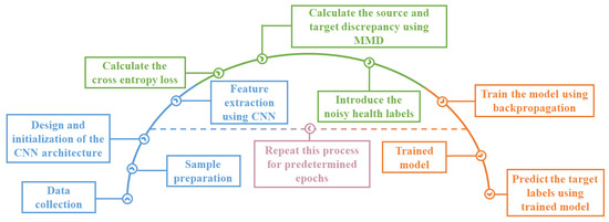
Figure 4.
The flowchart of the proposed deep learning model.
4. Result Analysis
4.1. Data Description
To validate the methodology proposed in this paper, two vibration datasets collected from the Bearing Data Centre of Case Western Reserve University (CWRU) and the Chair of Design and Drive Technology, Paderborn University, have been studied. The description of these datasets has been provided below.
4.1.1. CWRU Data Description
Vibration data acquired from four motor loads of 0, 1, 2 and 3 hp, corresponding to the motor speeds of 1797, 1772, 1750 and 1730 rpm, are utilized in this study. In this dataset, three types of bearing defects are implemented, i.e., inner race defect (IRD), outer race defect (ORD) and ball fault (BD). The faults having diameters in the range of 0.007, 0.014 and 0.021 inches were artificially induced in the drive-end (DE) bearings (SKF deep-groove ball bearings: 6205-2RS JEM) of the test rig motor at various locations. Hence, there are totally ten health classes considered in this study. For classification purpose, these ten health conditions with different fault locations (IRD, ORD and BD) and fault levels (0.007″, 0.014″ and 0.021″) are indicated using class labels 1 to 10 respectively. While acquiring data, a sampling frequency of 12 kHz was used.
4.1.2. Paderborn Data Description
In this dataset, the vibration data used for developing condition monitoring methods, which has been generated using a modular test rig, were devised and operated at the Paderborn University. Being a modular system, different defects are flexibly produced in the drive train for generating failure data using the experimental test rig. The test rig consists of the following modules: (a) an electric motor to drive the system, (b) a shaft for torque measurement, (c) the rolling bearing test module, (d) a flywheel module and (e) a load motor. A detailed description of the experimental setup is provided in [24].
The vibration signals collected in this dataset are sampled at a rate of 64 kHz. For ball bearings of type 6203 used in the experiments, artificial faults are generated by using different methods such as electrical discharge machining (EDM), drilling and manual electric engraving, etc. From the complete dataset comprising artificially induced faults and naturally occurring accelerated failure, the data corresponding to artificial damage are used in this study. Depending on the type of defect and the extent of damage produced, five health conditions are implemented in this study. To make the classification easier, these five conditions are denoted using labels 1 to 5, respectively. The details of each health class along with its corresponding test bearing description have been summarized in Table 1.

Table 1.
Description of health classes for Paderborn dataset.
From the entire dataset, the selection of the above-mentioned bearings helps to cover different artificial faults along with different levels of these faults. The healthy bearing in the above table was operated for a longer duration in more complex conditions and, hence, has been selected in this study. In this dataset, the bearing in the test rig is operated at four different operating conditions, as listed in Table 2. Each operating condition provides 80 s of vibration data (20 measurements of 4 s each) with a sampling frequency of 64 . In this study, multiple transfer tasks covering speed transfer, load torque transfer and radial force transfer are performed to evaluate the influence of change in operating conditions on the fault diagnosis performance. The experiments are targeted to evaluate the model’s performance when there is a distribution discrepancy between the training (source) and testing (target) data in terms of operating conditions.
Table 2.
Operating Conditions corresponding to the Paderborn Dataset.
4.2. Transfer Tasks
4.2.1. Transfer Tasks for CWRU Dataset
The specific details of each transfer task performed in this study are presented in Table 3. and indicate the number of the the samples for each health class under certain speed condition in source and target domains, respectively. In order to avoid additional complexity, the value of is kept equal to that of during the experiments. The dimensionality of each sample obtained from sequential acceleration data is indicated using . All transfer tasks consist of ten health classes (one healthy and nine faulty conditions). Since this dataset is comparably clean in terms of noise level, performing fault diagnosis on these data is straightforward. To make diagnosis more challenging, additional white Gaussian noise with signal-to-noise ratio (SNR) equal to 2 is added in the target domain data. The training of the model using clean source domain data and its testing on noisy target domain data helps in simulating industrial data environment to evaluate the model’s robustness. The standard network parameters used in this study are presented in Table 4. Multiple experiments were performed on a sample transfer task for determining the optimal values of certain parameters such as filter number, filter size, etc., while finalizing the network’s architecture.
Table 3.
Details of each transfer task for CWRU dataset.
Table 4.
Parameter specification in the proposed methodology.
4.2.2. Transfer Tasks for Paderborn Dataset
A detailed description of each transfer task performed on the Paderborn dataset is presented in Table 5. The information of standard network parameters for Paderborn dataset is also presented in Table 4. For simplicity, is again kept equal to that of during the experiments. Each task consists of five health classes (one healthy and four faulty conditions). Similarly to the experiments with the CWRU dataset, additional white Gaussian noise with SNR equal to 2 is added in the target domain data to make the task more challenging and evaluate the model’s performance in noisy environments. The network architecture is finalized using a sample task from the CWRU dataset and is directly used for performing experiments on the Paderborn dataset. All experimental results for both datasets are obtained using a PC with 16-GB RAM, Core i5 CPU and NVIDIA GeForce TX 2080 Ti. The experiments were executed in Python using Tensorflow on a GPU-based device.
Table 5.
Details of each transfer task for Paderborn dataset.
4.3. Experimental Results
4.3.1. Determination of Architectural Parameters
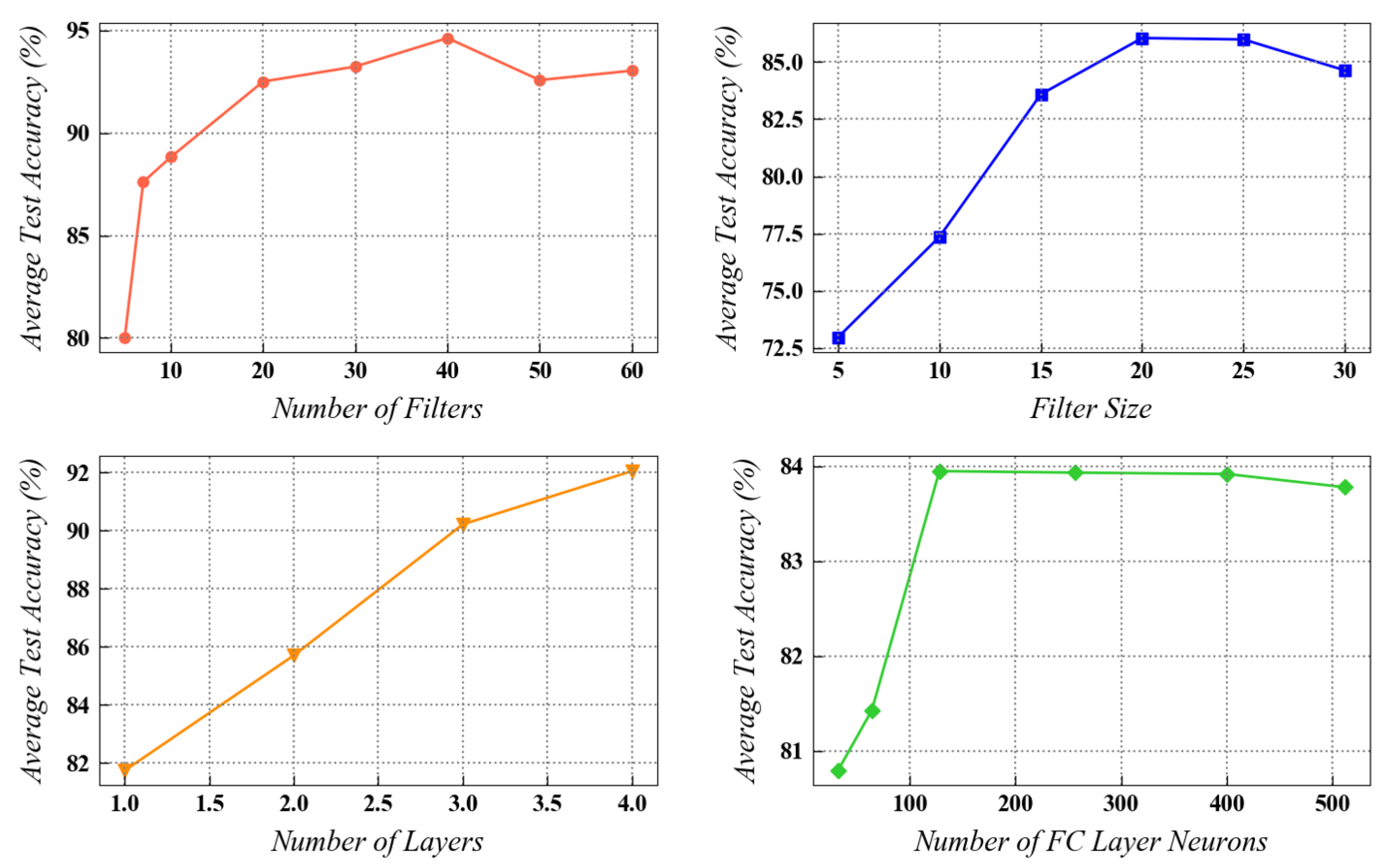
In this section, a sample task from the CWRU dataset is analyzed for finalizing the network architecture parameters used for performing the experiments. Four main hyperparameters, viz., the number of filters (), filter size (), number of convolutional layers and the number of neurons in the fully connected layer are mainly focused on, as they significantly affect the network optimization process in the fault diagnosis framework. These experimental tests for parameter finalization were performed using a 5-fold cross-validation approach. In the CWRU dataset, the transfer task from 0 hp to 3 hp, having the maximum domain discrepancy, is selected for running the tests in this section. The experimental results for the above-mentioned parameters are presented in Figure 5.

Figure 5.
The effect of four hyperparameters on the performance of the network in task of CWRU dataset.
As indicated in the Figure 5, a larger number of convolutional filters generally improves the model’s performance, resulting in higher test accuracies. A similar trend is observed while evaluating the effect of filter size on the model’s effectiveness. It was observed that the four double-convolutional layers provided higher accuracy compared to the three double-convolutional layers, but at the same time, significantly increased the computational load. Moreover, an increase in the number of fully connected neurons in the last layer of the network sharply improved the testing accuracy initially. After a certain point, the model’s performance started to deteriorate with an increase in the number of fully connected neurons due to possible overfitting. From the point of view of the network’s training efficiency and testing accuracy, a well-balanced trade-off needs to be achieved while selecting these parameters during actual implementation. In this study, a filter number of 40, filter size of 25, fully connected neurons equal to 128, and three double-convolutional layers were finalized for experimentation. This selection resulted in high testing accuracy along with acceptable computational time for network’s training.
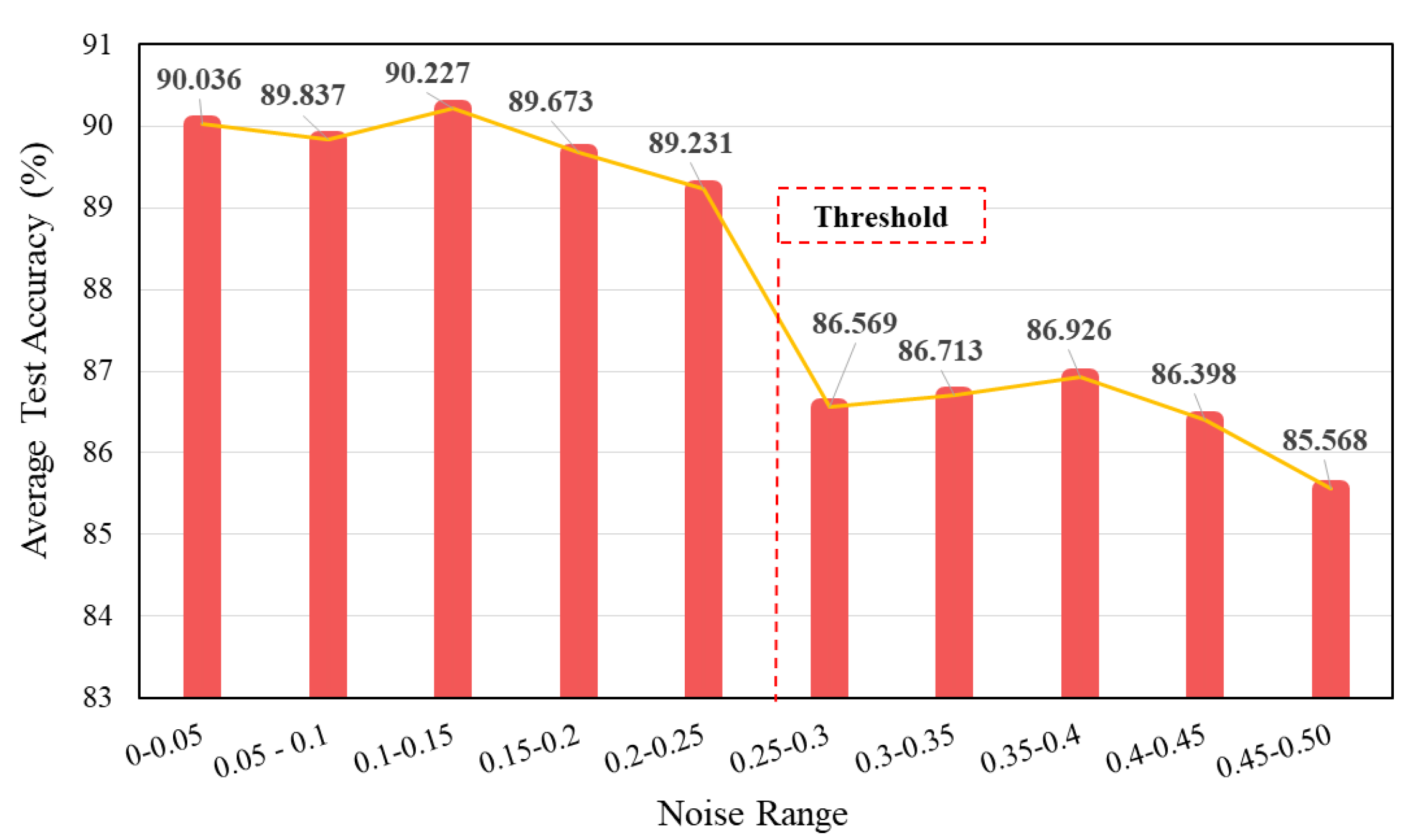
4.3.2. Selection of Optimal Noise Range for the Health Labels
For a deeper assessment of the proposed noisy label methodology, multiple experiments were performed by changing the extent of induced noise in small increments (0.05 increase) and then monitoring its effect on the test accuracy. A sample transfer task of 3 HP to 0 HP from the CWRU dataset, with a higher noise (SNR = −2) in the target data, was focused on. Higher noise level in the target domain data ensured a better evaluation of the method’s robustness and noise level selection. The test results are presented in Figure 6. It is clearly indicated in the figure that the addition of a smaller noise level in the health labels results in a significant increase in the model’s diagnostic performance. However, it should be noted that the introduction of a larger noise level above a certain threshold will reduce the testing accuracy of the model. For instance, when a higher noise level above 0.25 is injected into the health labels, a significant drop of almost 3% is observed in the testing accuracy. According to these experiments, an optimum level of noise, , was chosen, and a random noise value in the interval of [0, 0.25] was created for every epoch to obtain the needed noisy health labels for the experiments.

Figure 6.
Evaluating results for selecting the optimal noise range.
4.3.3. Compared Methods
In this section, a benchmarking study is performed for validating the effectiveness and reliability of the proposed noisy label-based domain adaptation method. The performance of the proposed method is compared with the following fault diagnosis tools:
- Deep Neural Network (DNN) [25] is a conventional deep learning method which consists of multiple FC layers stacked together for supervised learning. A network having four FC layers with 128 neurons in each layer is used for feature extraction. Finally, a softmax output layer with number of neurons equal to the number of health classes is adopted for classification.
- Support Vector Machine (SVM) [26] is a popular supervised machine learning algorithm traditionally used for classification as well as regression tasks. For establishing the SVM model, a structural risk minimization criterion adopted from the statistical learning theory is used for performing the desired task. Manually extracted features are provided as inputs to the model, along with the selection of an appropriate kernel.
- Transfer Component Analysis (TCA) [27] is a popular domain adaptation technique that tries to learn certain transfer components across the source and target domains and, hence, find a feature subspace in which similar data properties are encountered for the two domains with closer data distributions. On creating the new subspace, a standard SVM classifier is trained using the transformed source domain data for testing in the target domain.
- Joint Distribution Adaptation (JDA) [28] is a transfer learning approach that is useful when there exists a discrepancy between the marginal as well as the conditional distributions of the labeled source domain and unlabeled target domain data. JDA tries to formulate new feature representations for the domains by jointly adapting their marginal as well as conditional distributions during the dimensionality reduction process. These transformed representations are highly robust and effective for domain generalization.
- Balanced Distribution Adaptation (BDA) [29] is a transfer learning technique that targets the distribution adaptation problem by leveraging the importance of the marginal and conditional distribution discrepancies in an adaptive manner. It can also be effectively used in transfer learning problems having class imbalance scenarios.
- Geodesic Flow Kernel (GFK) [30] is a kernel-based unsupervised domain adaptation approach. It tackles the domain shift problem by integrating infinite subspaces that are used for mapping the geometric and statistical changes from the source domain data to the target domain data.
- Traditional Convolutional Neural Network (CNN) without any cross-domain adaptation, but having a similar architecture as the proposed method, is considered in this comparison study. The stacked convolutional and pooling layers are used for extracting meaningful features from the raw data signals. At the end, a fully connected layer is placed, which is followed by the softmax layer for classification. After training the model using only source domain data, the model is directly tested on target domain data.
- Convolutional Neural Network with MK-MMD [31]: The proposed method implements the CNN with cross-domain adaptation features. The maximum mean discrepancy metric is used for the alignment of source and target domain distributions.
4.3.4. Benchmarking Results and Performance Analysis
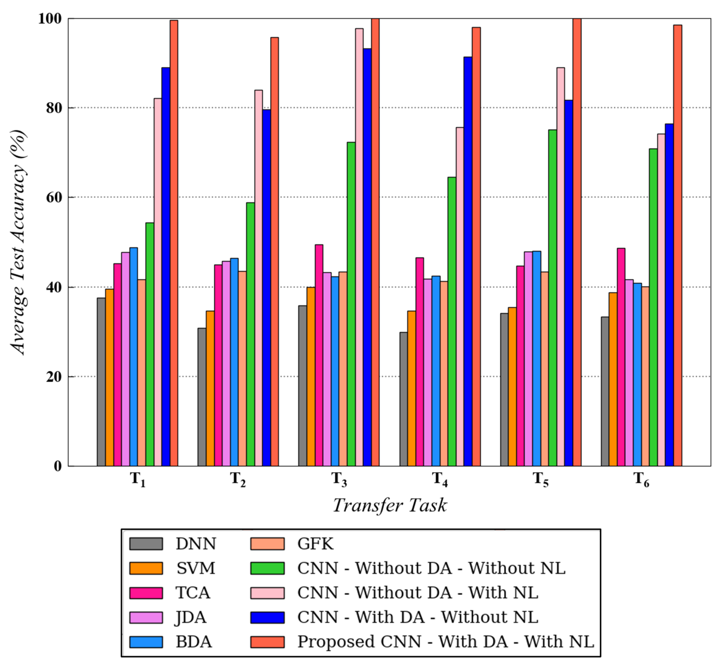
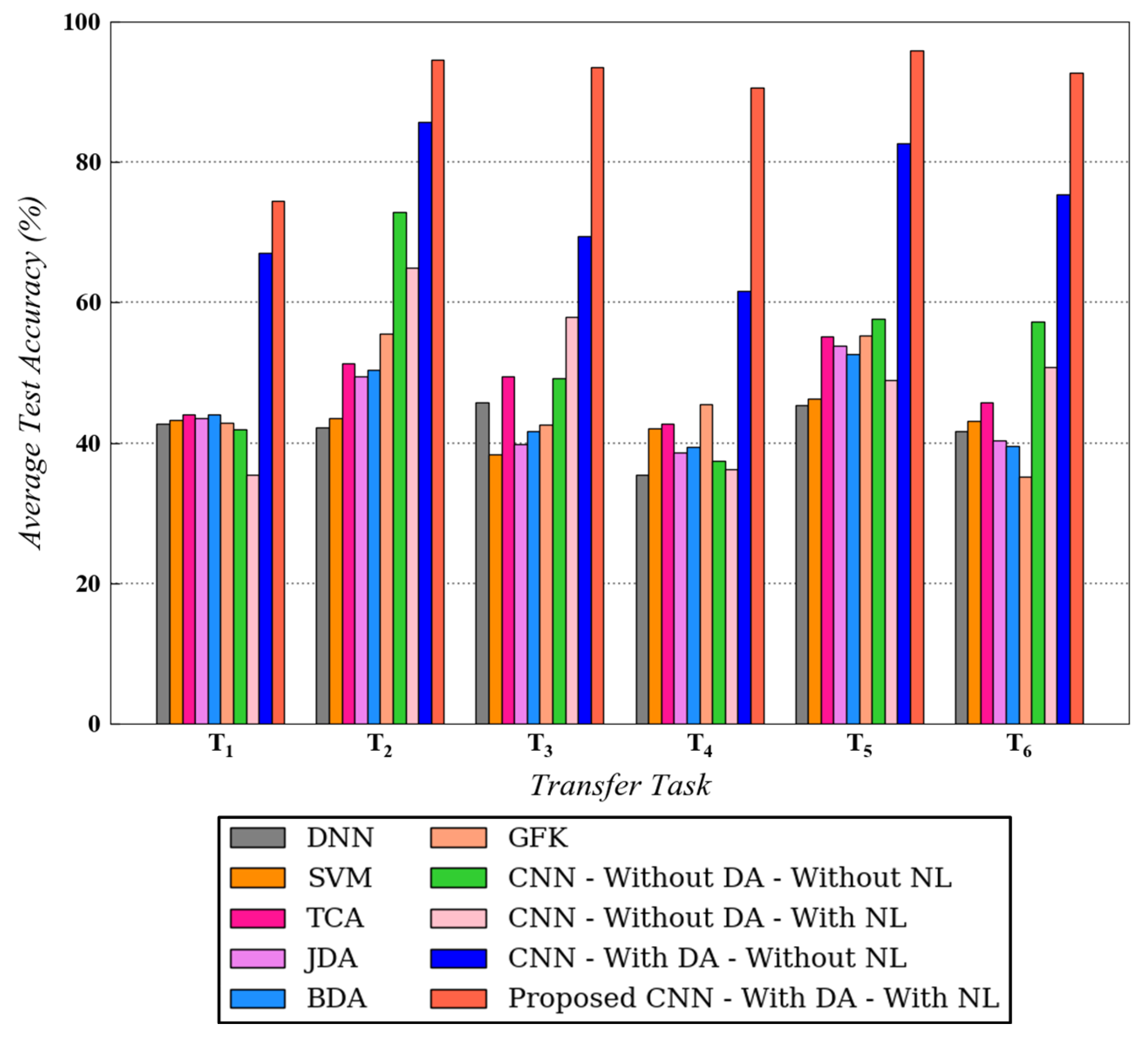
In this section, the experimental results for both datasets are explained in detail. Figure 7 and Figure 8 represent the benchmarking results for all six transfer tasks of CWRU and Paderborn dataset, respectively. For the tests on CWRU dataset, was used and for the Paderborn dataset, and was implemented. As depicted in both figures, the proposed methodology that uses noisy health labels in CNN-based cross-domain adaptation framework, achieves the best test accuracy for all transfer tasks. A similar trend in the results is observed for both datasets, which further strengthens the reliability and validates the effectiveness of the proposed method. Being a conventional machine learning method, SVM is not able to generalize well when it is trained on source domain data and directly tested on target domain data. In comparison to traditional methods, domain adaptation approaches such as TCA, JDA, BDA and GFK demonstrate a competitive performance for all tasks. However, the proposed method still outperforms these techniques.
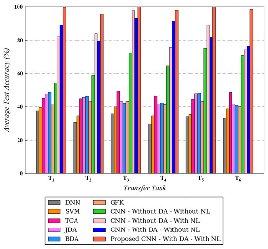
Figure 7.
Testing diagnosis performances on target domain for different transfer tasks using different algorithms on CWRU dataset. is used.
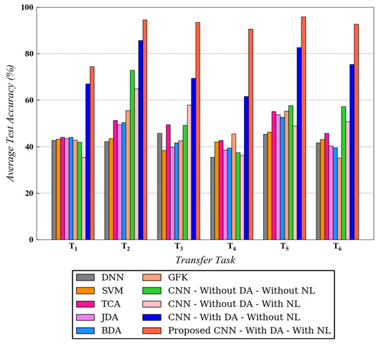
Figure 8.
Testing diagnosis performances on target domain for different transfer tasks using different algorithms on Paderborn dataset. is used.
Moreover, for the CWRU dataset, the results for CNN with domain adaptation and without noisy health labels and CNN without domain adaptation and with noisy health labels are always in proximity with the former surpassing the latter in certain tasks. However, for the Paderborn dataset, CNN with domain adaptation and without noisy health labels always produces a better diagnosis compared with CNN without domain adaptation (with or without noisy labels). For both the datasets, however, the introduction of noisy labels noticeably enhanced the performance of CNN-based domain adaptation model. The explanation for the performance enhancement after incorporating noisy labels is mainly originated from the regularization effect introduced by this technique during the model’s training process. Data augmentation is realized due to the availability of more valid training data samples with discrete health labels, resulting in stronger generalization ability. Correspondingly, a model augmentation effect is also generated, similar to other regularization techniques such as dropout.
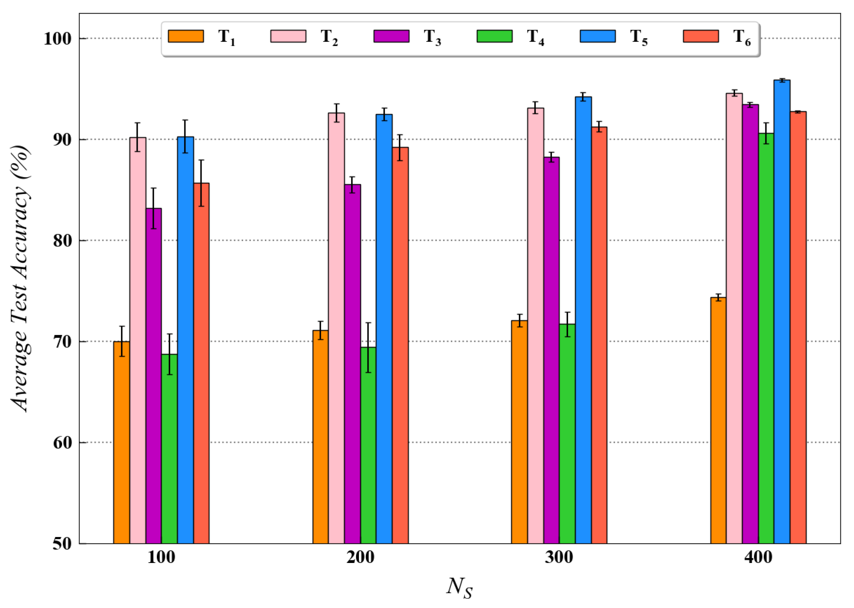
For quantitatively investigating the effect of training data size on the diagnostic performance of the proposed method, a performance analysis was also conducted in this study for both the datasets. The experimental results for this analysis are presented in Figure 9 and Figure 10 for the CWRU and Paderborn dataset, respectively. As observed in both figures, for each transfer task, the availability of a larger number of training data samples generally resulted in higher test accuracy. As stated in the literature, the performance of data-driven models usually improves when more data are available for training. The test results from this analysis are in accordance with the above statement; hence, they further validate our proposed approach.
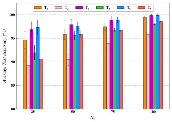
Figure 9.
Performance analysis results for various transfer tasks of CWRU dataset with different training data size using the proposed method.

Figure 10.
Performance analysis results for various transfer tasks of Paderborn dataset with different training data size using the proposed method.
The performance analysis results also depict the difficulty in minimizing the domain discrepancy for different transfer scenarios. For instance, in Figure 10, it can be observed that the testing accuracy, using the proposed method, is considerably less for task as compared to tasks and in different scenarios. The possible explanation for this result can be that domain discrepancy is usually higher in tasks involving transfer across different speed conditions (task ). Since the tasks and involve the difference in load and force conditions, respectively, the transfer of learned knowledge across the domains is comparatively easier for these tasks. Hence, the model’s performance under various transfer scenarios is well evaluated in this section.
It should be highlighted that a novel technique that integrates the noisy label algorithm into the domain adaptation framework is proposed in this paper for enhancing the cross-domain diagnosis performance. The use of noisy label algorithm, without any domain adaptation features, will unnecessarily reduce the model’s diagnostic performance due to additional noise in most of the cases. The simultaneous execution of domain adaptation and noisy label approach will ensure the extraction of domain-invariant features along with improved model generalization, ultimately resulting in performance enhancement. Hence, the effectiveness of the proposed methodology has been strongly validated in this section using different tests and comparisons with popular transfer learning methods in the literature.
4.4. Visualization of High-Level Features
In this section, the high-level feature representations, captured by the fully connected layer in the network, are visualized for better interpretation and understanding of the cross-domain fault diagnosis results. The popular t-distributed stochastic neighbor embedding (t-SNE) technique was utilized for visualizing the high-level fault features. Compared to other multi-dimensional scaling methods or techniques such as PCA, t-SNE provides additional flexibility while capturing the local data characteristics, improved ability to handle outliers and better illustration of minor changes in the data structure [32,33].
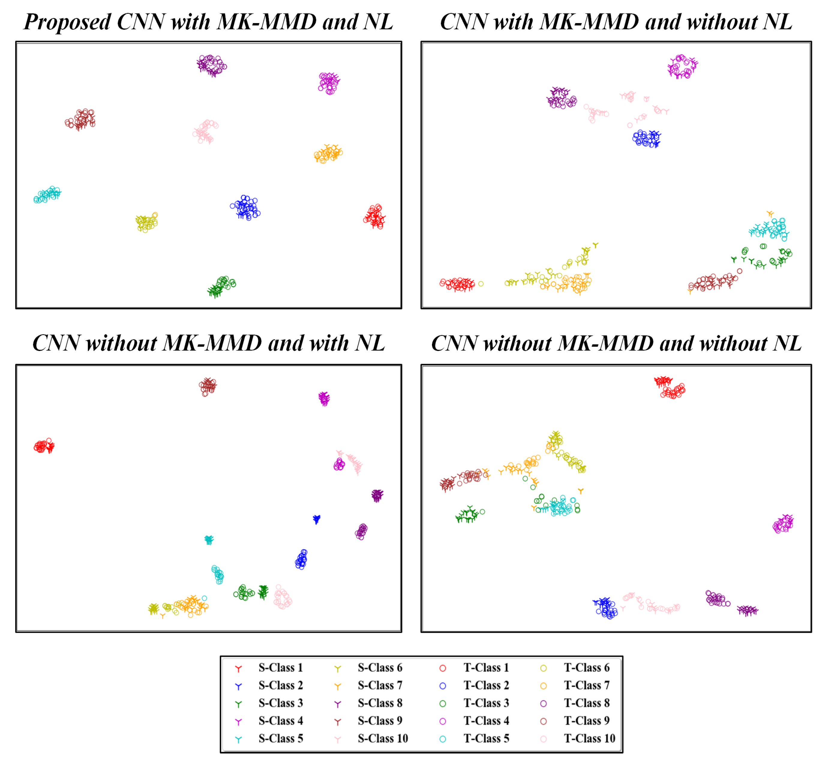
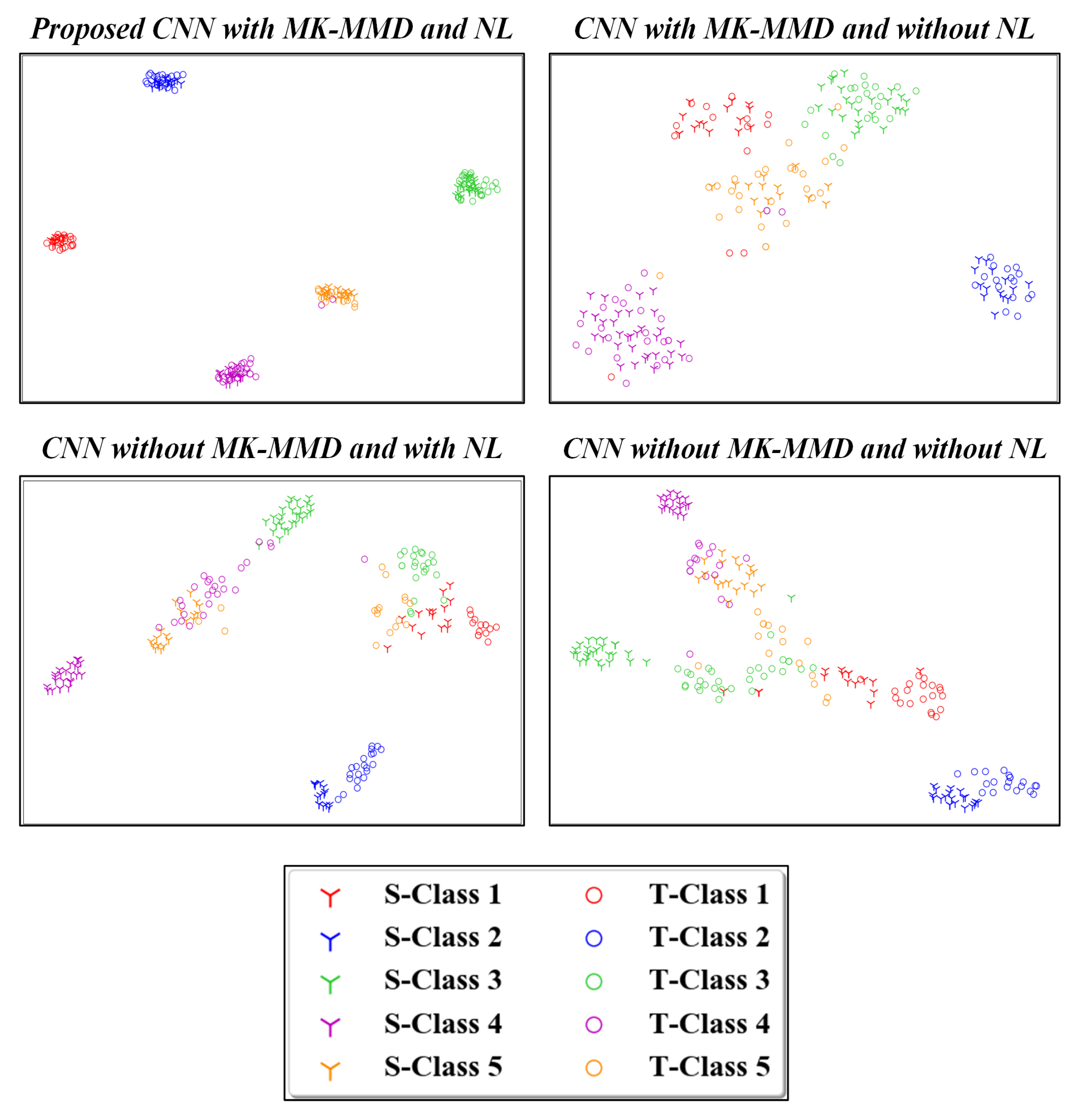
Figure 11 and Figure 12 present the two-dimensional plots of the learned high-level features obtained using four different methods for the transfer task: and from the CWRU and Paderborn dataset, respectively. As depicted, similar representations were obtained for both the studied datasets. When domain adaptation is not implemented, the learned features with the same health labels are clustered together as well, but there exist notable gaps between the data from the source and target domains. Furthermore, due to such domain discrepancies, the respective health condition labels of the source and target domains are mapped into far-off regions. This negatively impacts the generalization of learned feature knowledge from the source domain data to target domain data. After using the proposed idea of domain adaptation, the high-level feature representations with the same health labels from the source and target are well aligned to each other in the feature space. This demonstrates that the domain-invariant features are well extracted during network optimization. Correspondingly, the influence of the proposed noisy label algorithm on the domain adaptation performance is also depicted in Figure 11 and Figure 12. For the ten health classes in the CWRU dataset, a clear clustering effect was observed in Figure 11 using the proposed methodology. Similarly, five distinct clusters are also obtained for the Paderborn dataset, as seen in Figure 12. Hence, the effectiveness of the proposed noisy label-based domain adaptation method has been quantitatively validated in this section.

Figure 11.
Visualization results of high-level features in the fully connected layer by different methods. S- and T-denotes source and target domains, respectively. Task of the CWRU dataset is focused on.
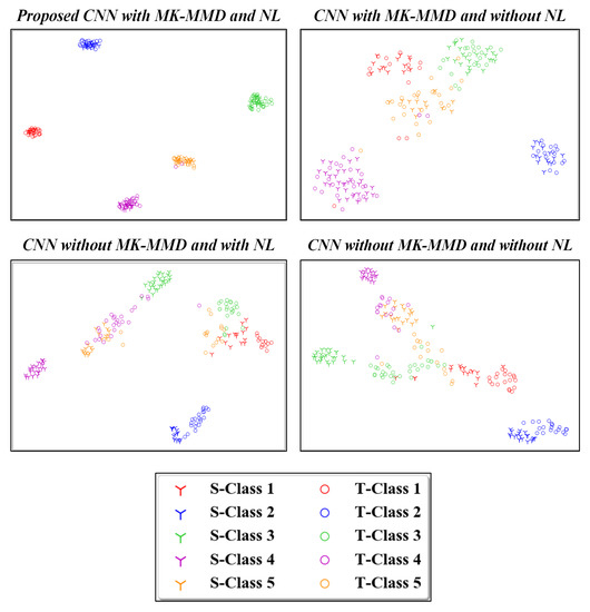
Figure 12.
Visualization results of high-level features in the fully connected layer by different methods. S- and T-denotes source and target domains, respectively. Task of the Paderborn dataset is focused on.
5. Conclusions
In this paper, a novel methodology for enhancing the performance of deep learning-based cross-domain fault diagnosis using noisy label algorithm is proposed. By injecting additional noise in the health condition labels of source data, the model’s generalization ability can be substantially enhanced as compared to its optimization using the conventional one-hot vector labels. Experiments on two popular rotating machinery datasets have been performed in this study to demonstrate the method’s usefulness. The presented findings indicate that the proposed technique can effectively extract domain-invariant features and generalize well on the target domain for better addressing the challenging cross-domain diagnosis problem. Although, promising results have been achieved in this paper, the proposed approach still relies on the availability of sufficient target domain data during the network’s training process. To address this limitation, future research work will be mainly concentrated on the development of efficient fault diagnosis models that require a limited amount of target domain data.
Author Contributions
Data curation, A.A.; Methodology, F.M.; Project administration, X.L. and J.L.; Writing—original draft, S.S. All authors have read and agreed to the published version of the manuscript.
Funding
This research received no external funding.
Institutional Review Board Statement
Not applicable.
Informed Consent Statement
Not applicable.
Data Availability Statement
Not applicable.
Conflicts of Interest
The authors declare no conflict of interest.
References
- Jia, F.; Lei, Y.; Guo, L.; Lin, J.; Xing, S. A neural network constructed by deep learning technique and its application to intelligent fault diagnosis of machines. Neurocomputing 2018, 272, 619–628. [Google Scholar] [CrossRef]
- Xiao, D.; Qin, C.; Yu, H.; Huang, Y.; Liu, C. Unsupervised deep representation learning for motor fault diagnosis by mutual information maximization. J. Intell. Manuf. 2020, 32, 377–391. [Google Scholar] [CrossRef]
- Li, X.; Jia, X.D.; Zhang, W.; Ma, H.; Luo, Z.; Li, X. Intelligent cross-machine fault diagnosis approach with deep auto-encoder and domain adaptation. Neurocomputing 2020, 383, 235–247. [Google Scholar] [CrossRef]
- Li, X.; Siahpour, S.; Lee, J.; Wang, Y.; Shi, J. Deep learning-based intelligent process monitoring of directed energy deposition in additive manufacturing with thermal images. Procedia Manuf. 2020, 48, 643–649. [Google Scholar] [CrossRef]
- Joshi, G.P.; Alenezi, F.; Thirumoorthy, G.; Dutta, A.K.; You, J. Ensemble of Deep Learning-Based Multimodal Remote Sensing Image Classification Model on Unmanned Aerial Vehicle Networks. Mathematics 2021, 9, 2984. [Google Scholar] [CrossRef]
- Shi, S.; Li, J.; Li, G.; Pan, P.; Liu, K. XPM: An Explainable Deep Reinforcement Learning Framework for Portfolio Management. In Proceedings of the 30th ACM International Conference on Information & Knowledge Management, Gold Coast, QLD, Australia, 1–5 November 2021; pp. 1661–1670. [Google Scholar]
- Siahpour, S.; Li, X.; Lee, J. Deep learning-based cross-sensor domain adaptation for fault diagnosis of electro-mechanical actuators. Int. J. Dyn. Control 2020, 8, 1054–1062. [Google Scholar] [CrossRef]
- Li, X.; Zhang, W.; Ma, H.; Luo, Z.; Li, X. Degradation Alignment in Remaining Useful Life Prediction Using Deep Cycle-Consistent Learning. IEEE Trans. Neural Netw. Learn. Syst. 2021, 1–12. [Google Scholar] [CrossRef]
- Zhang, W.; Li, X.; Ma, H.; Luo, Z.; Li, X. Federated learning for machinery fault diagnosis with dynamic validation and self-supervision. Knowl.-Based Syst. 2021, 213, 106679. [Google Scholar] [CrossRef]
- Hasan, M.J.; Kim, J.M. Bearing fault diagnosis under variable rotational speeds using stockwell transform-based vibration imaging and transfer learning. Appl. Sci. 2018, 8, 2357. [Google Scholar] [CrossRef] [Green Version]
- Ainapure, A.; Li, X.; Singh, J.; Yang, Q.; Lee, J. Deep learning-based cross-machine health identification method for vacuum pumps with domain adaptation. Procedia Manuf. 2020, 48, 1088–1093. [Google Scholar] [CrossRef]
- Zhang, Z.; Chen, H.; Li, S.; An, Z. Sparse filtering based domain adaptation for mechanical fault diagnosis. Neurocomputing 2020, 393, 101–111. [Google Scholar] [CrossRef]
- Li, S.; Liu, C.H.; Lin, Q.; Wen, Q.; Su, L.; Huang, G.; Ding, Z. Deep residual correction network for partial domain adaptation. IEEE Trans. Pattern Anal. Mach. Intell. 2020, 43, 2329–2344. [Google Scholar] [CrossRef] [PubMed] [Green Version]
- Zhang, W.; Li, X.; Ma, H.; Luo, Z.; Li, X. Open set domain adaptation in machinery fault diagnostics using instance-level weighted adversarial learning. IEEE Trans. Ind. Informatics 2021, 17, 7445–7455. [Google Scholar] [CrossRef]
- Wang, Q.; Michau, G.; Fink, O. Missing-class-robust domain adaptation by unilateral alignment. IEEE Trans. Ind. Electron. 2020, 68, 663–671. [Google Scholar] [CrossRef] [Green Version]
- Li, X.; Zhang, W.; Ma, H.; Luo, Z.; Li, X. Domain generalization in rotating machinery fault diagnostics using deep neural networks. Neurocomputing 2020, 403, 409–420. [Google Scholar] [CrossRef]
- Hu, T.; Tang, T.; Lin, R.; Chen, M.; Han, S.; Wu, J. A simple data augmentation algorithm and a self-adaptive convolutional architecture for few-shot fault diagnosis under different working conditions. Measurement 2020, 156, 107539. [Google Scholar] [CrossRef]
- Gao, X.; Deng, F.; Yue, X. Data augmentation in fault diagnosis based on the Wasserstein generative adversarial network with gradient penalty. Neurocomputing 2020, 396, 487–494. [Google Scholar] [CrossRef]
- Wang, Q.; Du, P.; Liu, X.; Yang, J.; Wang, G. Adversarial unsupervised domain adaptation for cross scenario waveform recognition. Signal Process. 2020, 171, 107526. [Google Scholar] [CrossRef]
- Kim, H.; Youn, B.D. A new parameter repurposing method for parameter transfer with small dataset and its application in fault diagnosis of rolling element bearings. IEEE Access 2019, 7, 46917–46930. [Google Scholar] [CrossRef]
- Gretton, A.; Borgwardt, K.M.; Rasch, M.J.; Schölkopf, B.; Smola, A. A kernel two-sample test. J. Mach. Learn. Res. 2012, 13, 723–773. [Google Scholar]
- Gretton, A.; Sejdinovic, D.; Strathmann, H.; Balakrishnan, S.; Pontil, M.; Fukumizu, K.; Sriperumbudur, B.K. Optimal kernel choice for large-scale two-sample tests. Adv. Neural Inf. Process. Syst. 2012, 25, 1205–1213. [Google Scholar]
- Ainapure, A.; Li, X.; Singh, J.; Yang, Q.; Lee, J. Enhancing intelligent cross-domain fault diagnosis performance on rotating machines with noisy health labels. Procedia Manuf. 2020, 48, 940–946. [Google Scholar] [CrossRef]
- Lessmeier, C.; Kimotho, J.K.; Zimmer, D.; Sextro, W. Condition monitoring of bearing damage in electromechanical drive systems by using motor current signals of electric motors: A benchmark data set for data-driven classification. In Proceedings of the European Conference of the Prognostics and Health Management Society, Bilbao, Spain, 5–8 July 2016; pp. 05–08. [Google Scholar]
- Chen, Z.; Deng, S.; Chen, X.; Li, C.; Sanchez, R.V.; Qin, H. Deep neural networks-based rolling bearing fault diagnosis. Microelectron. Reliab. 2017, 75, 327–333. [Google Scholar] [CrossRef]
- Yang, Y.; Yu, D.; Cheng, J. A fault diagnosis approach for roller bearing based on IMF envelope spectrum and SVM. Measurement 2007, 40, 943–950. [Google Scholar] [CrossRef]
- Pan, S.J.; Tsang, I.W.; Kwok, J.T.; Yang, Q. Domain adaptation via transfer component analysis. IEEE Trans. Neural Netw. 2010, 22, 199–210. [Google Scholar] [CrossRef] [Green Version]
- Long, M.; Wang, J.; Ding, G.; Sun, J.; Yu, P.S. Transfer feature learning with joint distribution adaptation. In Proceedings of the IEEE International Conference on Computer Vision, Sydney, NSW, Australia, 1–8 December 2013; pp. 2200–2207. [Google Scholar]
- Wang, J.; Chen, Y.; Hao, S.; Feng, W.; Shen, Z. Balanced distribution adaptation for transfer learning. In Proceedings of the 2017 IEEE International Conference on Data Mining (ICDM), New Orleans, LA, USA, 18–21 November 2017; pp. 1129–1134. [Google Scholar]
- Gong, B.; Shi, Y.; Sha, F.; Grauman, K. Geodesic flow kernel for unsupervised domain adaptation. In Proceedings of the 2012 IEEE Conference on Computer Vision and Pattern Recognition, Providence, RI, USA, 16–21 June 2012; pp. 2066–2073. [Google Scholar]
- Li, X.; Zhang, W.; Ding, Q.; Sun, J.Q. Multi-layer domain adaptation method for rolling bearing fault diagnosis. Signal Process. 2019, 157, 180–197. [Google Scholar] [CrossRef] [Green Version]
- Li, W.; Cerise, J.E.; Yang, Y.; Han, H. Application of t-SNE to human genetic data. J. Bioinform. Comput. Biol. 2017, 15, 1750017. [Google Scholar] [CrossRef]
- Van der Maaten, L.; Hinton, G. Visualizing data using t-SNE. J. Mach. Learn. Res. 2008, 9, 2579–2605. [Google Scholar]

Publisher’s Note: MDPI stays neutral with regard to jurisdictional claims in published maps and institutional affiliations. |
© 2022 by the authors. Licensee MDPI, Basel, Switzerland. This article is an open access article distributed under the terms and conditions of the Creative Commons Attribution (CC BY) license (https://creativecommons.org/licenses/by/4.0/).