Article

Coupling of Bio-Reactors to Increase Maximum Sustainable Yield

1
Institut de Recherche Pour Développement (IRD), UMMISCO, Sorbonne Université, F-93143 Bondy, France
2
Laboratoire d’Analyse Non Linéaire et Mathématiques Appliquées, Department of Mathematics, Faculty of Science, University of Abou Bekr Belkaïd, Tlemcen 13000, Algeria
*
Author to whom correspondence should be addressed.
Mathematics 2022, 10(4), 555; https://doi.org/10.3390/math10040555
Submission received: 17 December 2021 / Revised: 3 February 2022 / Accepted: 4 February 2022 / Published: 11 February 2022
(This article belongs to the Section Mathematical Biology)

Abstract

:
In the field of fisheries management, the objective is to obtain an optimal catch while maintaining the fishery resource at a sufficiently high level to avoid the extinction of the exploited species. In mathematical fishery models, the fishing effort that must be implemented to have a sustainable fishery with a maximum harvest rate in the long term is sought. This goal is called the “Maximum Sustainable Yield” (MSY). In the chemostat, the substrate can be seen as prey of which the predator is the product. MSY search is thus extended to the classical chemostat model with a Monod function. There exists a dilution rate that maximizes the product synthesis. The study is extended to the case of the gradostat with fast substrate and product exchanges between two coupled bioreactors. The existence of two time scales makes it possible to apply methods of aggregation of variables to derive a reduced model governing a few global variables describing the dynamics of the complete system at the slow time scale. The analysis of the mathematical aggregated model is performed. Existence of equilibria as well as local and global stability are studied. The overall product yield in the system of coupled bioreactors may be greater than the sum of the yields of the two uncoupled bioreactors, i.e., if they functioned without connection between them. The increase in product yield is all the more important as the distribution of the substrate and of the product is asymmetrical between the two coupled bioreactors. The model is applied to fish farming by considering the coupling of two breeding sites. Here again, the model makes it possible to find the fast fish exchanges that must be established between the two breeding basins to optimize the overall yield of the farm.

1. Introduction

A complex system is generally structured with at least two levels of organization: one corresponding to the overall system, and the other to that of the parts that constitute it. It may consist of identical coupled subsystems. The global system is also characterized by fast and slow time scales. Moreover, the coupling of several identical subsystems leads to considering a more complex mathematical model because it has a greater number of variables and parameters. It is therefore important to implement complexity reduction methods to study the dynamics of the global system. The class of dynamical system considered here has two parts and is written generically in the following form:
d x d τ = f ( x ) + ϵ s ( x )
where f ( x ) and s ( x ) represent respectively the fast and slow parts of the model depending on the state variables x. ϵ < < 1 is a small dimensionless parameter. τ is the fast time and t = ϵ τ the slow time. The previous model is called the complete system and consists of coupling several subsystems. The fast part corresponds to the exchanges between the subsystems supposed to take place at the fast time scale, while the slow part describes the internal dynamics specific to each isolated subsystem supposed to take place at the slow time scale. It is further assumed that the fast part is characterized by some constants of motion that constitute global variables, making it possible to describe the evolution of the full system at a slow time scale. The methods making it possible to obtain the reduced system governing the global variables at the slow time scale are the so-called “methods of aggregation of variables”. This terminology was introduced by [1]. The method of aggregation of variables consists in studying the fast system and showing that the fast variables quickly tend toward an attractor, such as a stable equilibrium. The “aggregated” model is obtained by making an approximation consisting in replacing the fast variables by their equilibrium values in the complete model. The reduced model thus obtained has fewer variables and is generally easier to manipulate than the original complete system. It can be used to study the dynamics of the complete model. Methods of aggregation of variables were described in several review articles, refs. [2,3,4] as well as [5]. The method just described above is called the “quick derivation method” and can be used when the resulting aggregated model is structurally stable and the small parameter ϵ is small enough. When the aggregated model is not structurally stable, it is necessary to use the Fenichel theorem [6]. The method of aggregation of variables was extended to various dynamical systems, such as discrete time models as well as partial differential equations [4] and nonautonomous systems [7].
When coupling several subsystems, one of the essential questions concerns the emergence of new properties at the global level compared to the properties of the isolated parts. There is dynamic emergence when the aggregated model has dynamic behaviors that its isolated parts do not have, for example the number of equilibria and their stability properties as well as certain types of periodic attractors, see for example [2]. In the context of this work, bioreactors are coupled and the question that arises concerns the emergence of new properties at the global level. Can the system of two coupled bioreactors have a productivity in terms of product synthesis greater than the sum of the productivities of each isolated reactor? This question will be addressed in this work. Such an approach with two timescales in the gradostat was already proposed in [5], looking for the conditions needed for coexistence of competitive consumers.
The first contribution focusing on the search for the optimal catch of a fished population dates back to the pioneering work of Schaefer [8]. The Maximum Sustainable Yield (MSY) makes it possible to exploit a marine species in a sustainable manner while avoiding causing its extinction. Much literature was devoted to the MSY, see the classic contribution [9]. In the corresponding chapter of the book [10], it is shown how to calculate the fishing effort required to maximize the catch for a logistically growing species in a stable environment. For over 50 years the MSY was used to make recommendations for the sustainable management of fisheries around the world [11].
However, the classic MSY approach finds limitations because it only considers a single exploited species. In reality, any marine species is part of a complex ecosystem with several species competing with it for the same resources and often prone to predation. Thus, various works were interested in determining the MSY in various types of fish communities, in particular prey–predator systems. A classic case concerns the Lotka–Volterra prey–predator model in which the prey alone, the predator alone, or both are exploited [11]. The approach was extended to the case of a functional response response exhibiting a saturation effect with the prey density, such as Holling type II. In this case, the joint exploitation of the prey and the predator leads to the predator extinction, while the MSY can only be obtained for exploitation of the prey [11]. MSY research was also extended to the classic Holling–Tanner prey–predator model with prey, predator and both prey and predator harvesting [12]. A prey–predator model with a ratio-dependent functional response was studied with both prey and predator harvesting for which the coexistence of the two species is possible at the MSY [13].
The MSY-type approach was extended to the case of any number of exploited species growing logistically and not prone to predation [14], as well as to a community of species with mutualistic interactions [15]. In reality, marine ecosystems are very complex involving many species at different trophic levels with multiple interactions of competition, predation, or cooperation. The search for the optimal catch of commercial species while taking into account this ecological complexity constitutes a challenge for the years to come. MSY research remains a useful tool for better fisheries management.
The present work is concerned with the problem of optimal yield in the chemostat. The chemostat can be considered as a controlled medium into which a substrate (the prey) is injected and is consumed by the product (the predator). The aim of this work is to find the dilution rate that maximizes the product yield. In other words, the conditions allowing to obtain the “MSY” in mathematical models of chemostat and coupled bioreactors are sought. The work begins with the simplest mathematical model of chemostat, the classical model with Monod function. Mathematical models of chemostat are found in the classic books [16,17]. Then, the approach is extended to the case of the coupling of two bioreactors connected by fast exchanges of substrate and product. In a chemostat, a single product can be synthesized from a single substrate. In the case of two products synthesized from a substrate, one of the two products is led to extinction. This is by analogy the principle of exclusion in ecology, a single ecological niche allows only one species to exploit it. The gradostat was studied in particular to find the conditions for the coexistence of two competitors in a system of two coupled chemostats [18,19,20]. The method was extended to the case of N > 2 coupled chemostats to search for the coexistence of several competitors from a single resource [16,17].
The work is organized as follows. The first section presents the methods, especially how to calculate the optimal dilution rate in the classical model of the chemostat by considering the Monod function as well as extension to the system of two coupled bioreactors. Conditions of existence of equilibria and their global stability for the gradostat are given. The next section is devoted to results and discussion. First, examples of potential applications that concern the coupling of 2 chemostats are considered. Especially sought are the conditions allowing to have at MSY a product yield of the system of coupled bioreactors greater than the sum of those of the two isolated bioreactors. Next, a potential application to fish farming is presented for which a similar result is shown. The manuscript ends with a conclusion and perspectives.

2. Methods

2.1. The Minimal Model of the Chemostat and the MSY

The existence of a dilution rate that optimizes product synthesis is already known [21]. However, the problem is formulated by analogy with the fishing models in terms of MSY. The following “minimal” chemostat model is considered, as presented in [16]:
d s d t = D s i n D s μ m a x s x k + s
d x d t = μ m a x s x k + s D x
The variables are the substrate and product concentrations, respectively s ( t ) and x ( t ) in (mass/volume), i.e., ( M . V 1 ), at time t. D is the dilution rate in (1/time), i.e., ( T 1 ). s i n is the substrate input concentration in ( M . V 1 ). D s i n is the input substrate flow in ( M . V 1 . T 1 ), which must be homogeneous with the left-hand side of the equations. The Monod production function is considered, μ ( s ) = μ m a x s k + s . μ m a x is the maximum value of μ ( s ) and k is the “semi-saturation” constant. The mathematical study of this model is classic with the main following results [16]. There exists a “washout” equilibrium ( s i n , 0 ) and an equilibrium with biomass ( s , x ) checking s + x = s i n . If D < μ ( s i n ) , the washout equilibrium is Globally Asymptotically Stable (GAS) in the strictly positive orthant, or D μ ( s i n ) , the washout equilibrium is unstable while the equilibrium with biomass is GAS in the strictly positive orthant.
The equilibrium with biomass is the following:
s = D k ( μ m a x D )
x = s i n D k ( μ m a x D )
To have a positive substrate equilibrium, D < μ m a x is needed. The equilibrium substrate does not depend on the input substrate flux. At equilibrium, the output product flux is:
Y = D x = D s i n D 2 k ( μ m a x D )
By fixing all the parameters except the dilution rate, the output product flux can be seen as a function of D. This function presents a maximum in the domain where the equilibrium with biomass is GAS. This function is positive between 0 and D 0 = μ ( s i n ) = μ m a x s i n s i n + k . In this domain, it shows a maximum when:
d Y ( D ) d D = s i n 2 k μ m a x D k D 2 ( μ m a x D ) 2 = 0
which leads to the following second degree equation:
( s i n + k ) D 2 2 μ m a x ( s i n + k ) D + s i n μ m a x 2 = 0
with a positive discriminant δ = μ m a x 2 k ( s i n + k ) and a maximum in the domain 0 < D < μ m a x for the following dilution rate:
D M S Y = μ m a x ( s i n + k ) μ m a x 2 k ( s i n + k ) s i n + k
or else:
D M S Y = μ m a x 1 k ( s i n + k )
Consequently, the yield at MSY, Y M S Y = Y ( D M S Y ) reads as follows:
Y M S Y = μ m a x s i n + k k 2

2.2. The Model of a System of Two Coupled Bioreactors with Fast Substrate and Product Exchanges

The coupling of two bioreactors with fast exchanges is going to be considered in this section.

2.2.1. Presentation of the Complete Model

A system of two identical bioreactors with substrate s 1 ( t ) (resp. s 2 ( t ) ) and product x 1 ( t ) (resp. x 2 ( t ) ) concentrations in bioreactors 1 and 2 at time t is considered. The two bioreactors are connected to each other.
The complete system reads as follows:
d s 1 d τ = ( m 2 s 2 m 1 s 1 + I 1 s i n 1 E 1 s o u t 1 ) + ϵ ( D s i n D s 1 μ s 1 x 1 k + s 1 )
d s 2 d τ = ( m 1 s 1 m 2 s 2 + I 2 s i n 2 E 2 s o u t 2 ) + ϵ ( D s i n D s 2 μ s 2 x 2 k + s 2 )
d x 1 d τ = ( m 2 x 2 m 1 x 1 ) + ϵ ( μ s 1 x 1 k + s 1 D x 1 )
d x 2 d τ = ( m 1 x 1 m 2 x 2 ) + ϵ ( μ s 2 x 2 k + s 2 D x 2 )
ϵ < < 1 is a small dimensionless parameter. τ is the fast time and t = ϵ τ the slow time. m 1 (resp. m 2 ) is a constant rate of substrate and product exchange from chemostat 1 to chemostat 2 (resp. from chemostat 2 to chemostat 1) in ( T 1 ). These exchange flows between bioreactors are supposed to transport the substrate and the product from one reactor to another and therefore vary the concentrations inside the reactors. Parameters I i and E i represent positive and constant substrate input and output rates in ( T 1 ). These flows are set up to ensure a constant volume in each bioreactor. s i n i (resp. s o u t i ) is the input (resp. output) substrate concentration for bioreactor i, i = 1 , 2 in ( M . V 1 ). A classical Monod function with μ and k as reaction parameters is still considered. For simplicity, μ = μ m a x is used as notation. s i n still represents the input substrate concentration. The substrate and product flow out from the two bioreactors at the same constant dilution rate D. Figure 1 shows a diagram of the system of two tanks connected to each other by fast substrate and products exchanges at constant rates m 1 and m 2 .
The fast system is obtained when ϵ = 0 :
d s 1 d τ = ( m 2 s 2 m 1 s 1 + I 1 s i n 1 E 1 s o u t 1 )
d s 2 d τ = ( m 1 s 1 m 2 s 2 + I 2 s i n 2 E 2 s o u t 2 )
d x 1 d τ = ( m 2 x 2 m 1 x 1 )
d x 2 d τ = ( m 1 x 1 m 2 x 2 )
The input and output flows are assumed to keep the volumes and concentrations constant at the fast time in each bioreactor. First, the product particles are assumed to be large enough to remain in the bioreactors when fast output flows at rate E i are made. A filtration system at the exit of each tank prevents product particles from exiting but not substrate ones, which could be smaller. In the event that it would be impossible to filter the substrate, the output concentration would simply be s o u t i = s i . If it would possible to completely filter the substrate from the output flow, it would be s o u t i = 0 . Intermediate situations could also be considered.
Consider the case m 1 > m 2 . Initially the two reactors have the same volume V. For simplicity, V = 1 is chosen. Under these conditions, the exchange flow from the first chemostat to the second is greater than the reverse flow. Under these conditions, the reactor 1 gradually empties while filling the second. As mentioned earlier, input and output flows with the exterior are set to keep the volume of each reactor constant. In the case where the filtration of the substrate is total, that is to say when the output flows are only water, the following choice must be made:
I 1 = ( m 1 m 2 ) , E 1 = 0 , s i n 1 = 0
Indeed, since the first reactor empties, it is necessary to establish an input flow of water and remove the output flow. Since it is only water, the chosen substrate input concentration is zero. Similarly for the second reactor, the next choice is needed:
I 2 = 0 , E 2 = ( m 1 m 2 ) , s o u t 1 = 0
The above example corresponds to perfect filtering. In the more general case where it is impossible to completely filter the substrate, it is necessary to seek the input and output flows that guarantee both to keep the volume of each reactor constant as well as the substrate concentration in each reactor. In any case, a water input flow can be set to keep constant the volume of the reactor that empties, here the first one. On the other hand, if the substrate filtration is totally ineffective, the output flow of the second reactor to maintain its constant volume will include a certain concentration of substrate. This question is not approached in much detail in this work and will be the subject of a future study. The case m 1 < m 2 is symmetric.

2.2.2. Reduction of the Complete Model

The complete model takes into account two time scales. The use of timescale separation method allows one to derive a reduced and global model easier to analyze and simulate than the original complete model. Time separation methods are presented in the early reference [22]. Methods of aggregation of variables are defined in [1], and presented in more details in [3,4]. The quick derivation method is used in this section [2]. The fast system is obtained when ϵ = 0 . Assuming that input and output flows (at the fast time scale) keep the volumes and total substrate concentration constant, the fast system gets simplified to become:
d s 1 d τ = ( m 2 s 2 m 1 s 1 )
d s 2 d τ = ( m 1 s 1 m 2 s 2 )
d x 1 d τ = ( m 2 x 2 m 1 x 1 )
d x 2 d τ = ( m 1 x 1 m 2 x 2 )
Let total substrate concentration be s ( t ) = s 1 ( t ) + s 2 ( t ) as well as total product concentration, x ( t ) = x 1 ( t ) + x 2 ( t ) . The total substrate and product concentrations are first integrals for the previous fast system. As a result, the total substrate and product concentrations do not vary at the fast time scale. They define global variables varying at the slow time scale. The fast system is simplified as two uncoupled equations:
d s 1 d τ = m 2 ( s s 1 ) m 1 s 1
d x 1 d τ = m 2 ( x x 1 ) m 1 x 1
For any value of the “constant” s, there exists a fast and stable substrate equilibrium as follows:
s 1 = u s = m 2 m 1 + m 2 s
s 2 = ( 1 u ) s = m 1 m 1 + m 2 s
where u is the proportion of substrate in chemostat 1 at the fast equilibrium. Similarly for the product x 1 = u x and x 2 = ( 1 u ) x . When m 1 = m 2 , the distribution of the substrate between the two bioreactors is symmetrical and u = 0.5 . Otherwise, there is an asymmetrical distribution of the substrate and product in the bioreactors with constant volume. After substitution of the fast equilibrium into the complete model, by adding the equations of the substrate and the product two by two and by using the slow time, the following “aggregated” model is obtained:
d s d t = 2 D s i n D s μ u 2 s x k + u s μ ( 1 u ) 2 s x k + ( 1 u ) s
d x d t = μ u 2 s x k + u s + μ ( 1 u ) 2 s x k + ( 1 u ) s D x
This aggregated model is reduced and simpler than the complete model and can be used to understand and simulate the dynamics of the system when the small parameter is small enough and when the resulting aggregated model is structurally stable, which is the case here [3,4].

2.2.3. Existence and Positivity of Solutions of the Aggregated Model

The previous aggregated model is original because it has two production terms with different denominators except in the very special cases where u = 0 , 1 or 0.5 . With the exception of these previous special cases, the aggregated mathematical model is different from the mathematical models of each bioreactor and there is formal emergence.
Theorem 1.
The solutions of the system are non-negative for any positive or null initial conditions.
Proof. 
Note
U ( s ) = μ u 2 s k + u s + μ ( 1 u ) 2 s k + ( 1 u ) s .
Once a solution enters the plan
Ω = { ( s , x ) R 2 | s 0 , x 0 } .
it stays there forever. Indeed, by continuity of the solutions (aggregated model), each solution must take the value 0 before taking a negative value. if x = 0 for a value of t = t 1 > 0 , then, from the second equation of the aggregated system, x ( t 1 ) = 0 , and therefore x is nondecreasing in t 1 , which means that x is at least nondecreasing at x = 0 , this excludes the possibility that x takes a negative value.
Again, when s = 0 , the next expression holds:
s ( t ) = 2 D s s i n > 0 ,
since s 0 , and U ( 0 ) = 0 . s is therefore an increasing function at s = 0 . When x = 0 , s ( t ) = 2 D s i n D s , again for s = 0 , s ( t ) = 2 D s i n > 0 and therefore, s is increasing at x = 0 . Thus, the solutions of the aggregated system are non-negative for all t > 0 . □
Theorem 2.
Any positive solution of the aggregated model is bounded for any non-negative condition.
Proof. 
Consider function
V ( t ) = V ( s ( t ) , x ( t ) ) = s ( t ) + x ( t )
It is clear that V ( 0 , 0 ) = 0 , V ( s ( t ) , x ( t ) ) 0 for t 0 and V ( t ) when s ( t ) , x ( t ) . The derivative of function V along the solution of the aggregated model is:
V = 2 D s i n D s ( t ) a U ( s ( t ) ) x ( t ) + a U ( s ( t ) ) x ( t ) D x ( t ) = 2 D s i n D ( s ( t ) + x ( t ) ) 2 D s i n D V ( t ) .
Thus, outside the region delimited by the axes of the positive quadrant and the surface s + x = 2 s i n , V ( t ) is negative definite. So V is a Lyapunov function. Now, the conclusion follows from Burton’s Theorem [23], (see Appendix A) with W ( t , X ( t ) ) = s ( t ) , Q ( t , X ( t ) ) = V ( t ) , and U ˜ = 2 s i n . □

2.2.4. Equilibrium Solutions

The reduced model has a washout equilibrium ( 2 s i n , 0 ) and an interior equilibrium ( s , x ) . The nontrivial equilibrium ( s , x ) verifies:
( s + x ) = 2 s i n
Therefore, at equilibrium, the yield of product is simply given by the next expression:
D x = 2 D s i n D s
where s is solution of the next equation:
μ u 2 s k + u s + μ ( 1 u ) 2 s k + ( 1 u ) s = D
s is the positive root of the equation
F ( s ) = α 1 s 2 + α 2 s α 3 = 0
where the coefficients are
  • α 1 = ( μ D ) u ( 1 u ) ,
  • α 2 = μ k ( u 2 + ( 1 u ) 2 ) k D ,
  • α 3 = D k 2 .
As by hypothesis α 1 > 0 , by Descartes’ rule of signs, it follows that there is one positive real root of (30) given by
s = μ k ( u 2 + ( 1 u ) 2 ) + k D + Δ 2 ( μ D ) u ( 1 u )
where the discriminant Δ of the polynomial F is given by Δ = [ μ k ( u 2 + ( 1 u ) 2 ) k D ] 2 + 4 D k 2 ( μ D ) u ( 1 u ) .
This equilibrium is positive if
D < μ 2 u 2 s i n ( k + 2 u s i n ) + μ 2 ( 1 u ) 2 s i n ( k + 2 ( 1 u ) s i n ) = U ( 2 s i n )
Let J be the Jacobian matrix:
J = D μ k u 2 x ( k + u s ) 2 μ k ( 1 u ) 2 x ( k + ( 1 u ) s ) 2 μ u 2 s ( k + u s ) μ ( 1 u ) 2 s ( k + ( 1 u ) s ) μ k u 2 x ( k + u s ) 2 + μ k ( 1 u ) 2 x ( k + ( 1 u ) s ) 2 D + μ u 2 s ( k + u s ) + μ ( 1 u ) 2 s ( k + ( 1 u ) s )
For the washout equilibrium ( 2 s i n , 0 ) , the Jacobian reads:
J 0 = D μ 2 u 2 s i n ( k + 2 u s i n ) μ 2 ( 1 u ) 2 s i n ( k + 2 ( 1 u ) s i n ) 0 D + μ 2 u 2 s i n ( k + 2 u s i n ) + μ 2 ( 1 u ) 2 s i n ( k + 2 ( 1 u ) s i n )
One eigenvalue D is negative, and the other one is negative when:
D > μ 2 u 2 s i n ( k + 2 u s i n ) + μ 2 ( 1 u ) 2 s i n ( k + 2 ( 1 u ) s i n )
For the interior equilibrium ( s , x ) , the Jacobian reads as follows:
J = D μ k u 2 x ( k + u s ) 2 μ k ( 1 u ) 2 x ( k + ( 1 u ) s ) 2 μ u 2 s k + u s μ ( 1 u ) 2 s k + ( 1 u ) s μ k u 2 x ( k + u s ) 2 + μ k ( 1 u ) 2 x ( k + ( 1 u ) s ) 2 0
When the interior equilibrium ( s , x ) is strictly positive, the trace of the Jacobian is negative and the determinant is positive, and consequently, the interior equilibrium is locally asymptotically stable.

2.2.5. Global Stability

Theorem 3.
The washout equilibrium ( 2 s i n , 0 ) is globally asymptotically stable provided condition (32) holds.
Proof. 
From second equation, it is clear that if (32) holds, then lim t x ( t ) = 0 when t . It suffices to show that s ( t ) 2 s i n as t when the condition (32) is met. □
Consider function
V ( t ) = V ( s ( t ) , x ( t ) ) = s ( t ) + x ( t ) .
Clearly, V ( 0 , 0 ) = 0 and V ( s ( t ) , x ( t ) ) > 0 for s > 0 , x > 0 and along solutions of the aggregated model, the derivative reads as follows
V ( t ) = 2 D s i n D s ( t ) a U ( s ( t ) ) x ( t ) D x ( t ) + a U ( s ( t ) ) x ( t ) = 2 D s i n D ( s ( t ) + x ( t ) )
i.e., V ( t ) = D V ( t ) + 2 D s i n , then
V ( t ) = V ( 0 ) e D t + 2 s i n
thus, lim t V ( t ) = lim t ( s ( t ) + x ( t ) ) = 2 s i n , as lim t x ( t ) = 0 , showing the result.
Theorem 4.
The positive equilibrium of the aggregated model is globally asymptotically stable if condition (31) is met.
Proof. 
Consider function
V ( t ) = V ( s ( t ) , x ( t ) ) = 1 2 ( 2 s i n s x ) 2 + α x x x l o g x x .
It is obvious that V ( s , x ) = 0 , and V ( s , x ) > 0 for s > s and x > x . The derivative of V along solutions of the aggregated model is given by the next expression:
V = ( 2 s i n s x ) ( s x ) + α ( x x ) x x = ( 2 s i n s x ) 2 s i n D D s U ( s ) x + U ( s ) x D x + α ( x x ) ( U ( s ) D ) = D ( 2 s i n s x ) 2 + α ( x x ) ( U ( s ) D ) = D [ ( s s ) + ( x x ) ] 2 + α U ( s ) U ( s ) s s ( s s ) ( x x ) = D ( s s ) 2 + ( x x ) 2 + 2 α D U ( s ) U ( s ) s s ( s s ) ( x x )
Here 2 s i n = s + x is used. The expression on the right between braces of the last equation is of the form X 2 + B X Y + Y 2 = 0 and the condition for it to be positive definite is B 2 < 4 . Define X = x x , Y = y y and B = 2 α D U ( s ) U ( s ) s s , leading to,
D ( s s ) 2 + ( x x ) 2 + ( 2 α D U ( s ) U ( s ) s s ) ( s s ) ( x x )
is positive definite provided
2 α D U ( s ) U ( s ) s s 2 < 4 ,
that is to say
0 < α D U ( s ) U ( s ) s s < 4
or
α D U ( s ) U ( s ) s s = = α μ k D u 2 ( k + u s ) ( k + u s ) + ( 1 u ) 2 ( k + ( 1 u ) s ) ( k + ( 1 u ) s )
which is positive. There remains the other inequality:
α D U ( s ) U ( s ) s s = α μ k D u 2 ( k + u s ) ( k + u s ) + ( 1 u ) 2 ( k + ( 1 u ) s ) ( k + ( 1 u ) s ) α μ D u 2 k + u s + ( 1 u ) 2 k + ( 1 u ) s α μ D u s + 1 u s = α μ D s
As this last inequality is checked for all s, the condition is
α μ D s < 4
in other words: if α < 4 D s μ the previous function is positive definite. □
Choose 0 α < 4 D s μ , then V < 0 . So V is a Lyapunov function, and therefore the equilibrium point is GAS.

3. Results and Discussion

3.1. Maximum Sustainable Yield for the Chemostat

Figure 2 shows the yield Y ( D ) with a maximum for a value of the dilution rate D M S Y corresponding to the MSY. In this example, the maximum Yield is Y M S Y = Y ( D M S Y ) = 0.84 for a dilution rate D M S Y of about 0.8 . Under these conditions, to optimize the product yield, it is needed to choose a dilution rate equal to D M S Y .

3.2. Maximum Sustainable Yield for the System of Two Coupled Bioreactors

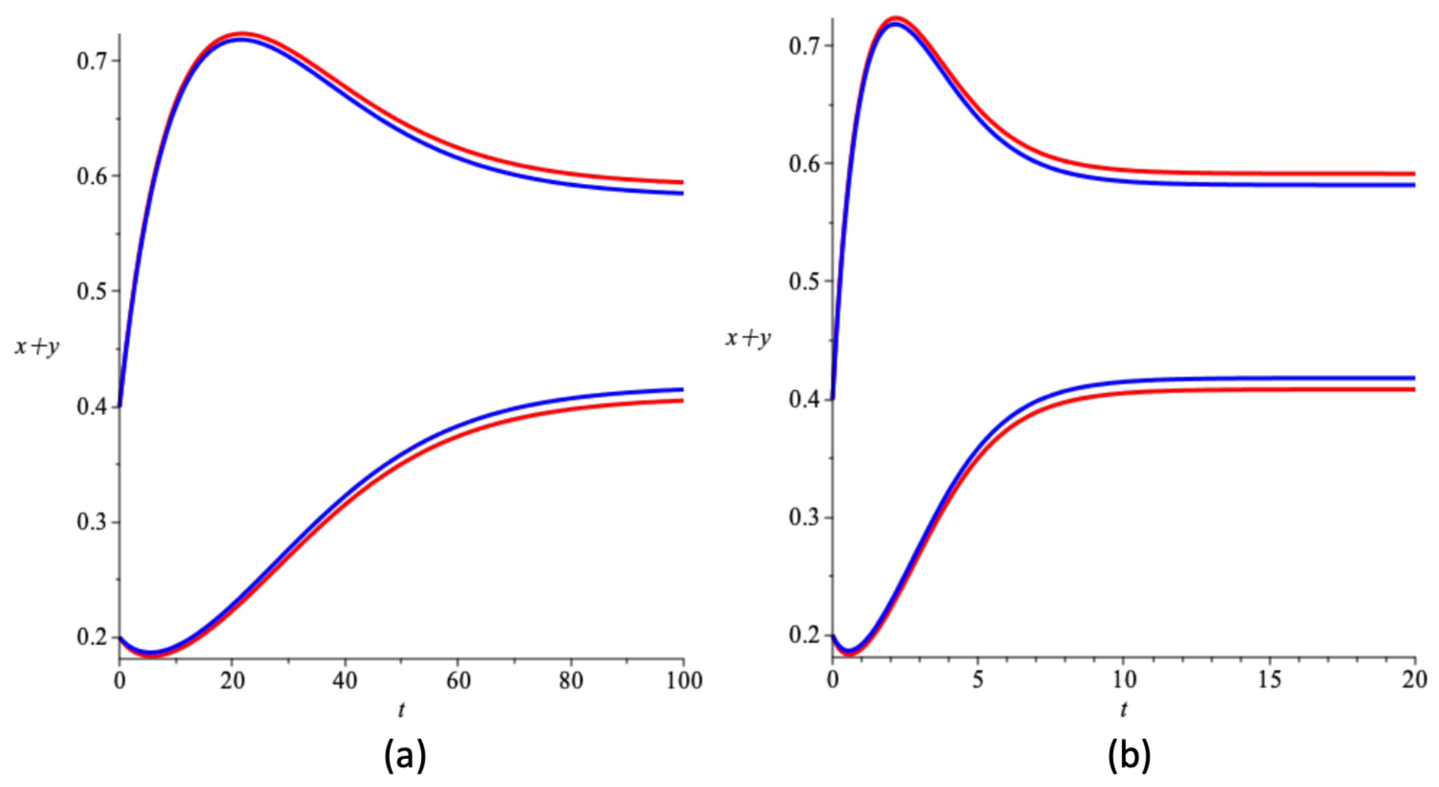
Figure 3 shows the comparison of the complete (blue) and aggregated (red) solutions for (a) m 1 = 0.3 , m 2 = 0.7 , ϵ = 0.1 and for (b) m 1 = 3 , m 2 = 7 , ϵ = 1 , and other parameters, s i n = 0.5 , μ = 8.5 and k = 2.5 . Similar initial conditions for complete model s 1 ( 0 ) = s 2 ( 0 ) = 0.2 , x 1 ( 0 ) = x 2 ( 0 ) = 0.1 , and aggregated, s ( 0 ) = 0.4 , x ( 0 ) = 0.2 are chosen. Figure 3a shows that for a reasonable value of the small parameter, ϵ = 0.1 , the solutions of the complete model and of the aggregated model remain very close. Figure 3b shows that even for ϵ = 1 , as soon as the exchange rates between chemostats are greater (by an order of magnitude) than other parameters of the slow part of the complete model, the solutions of the complete and aggregated models still remain close to each other.
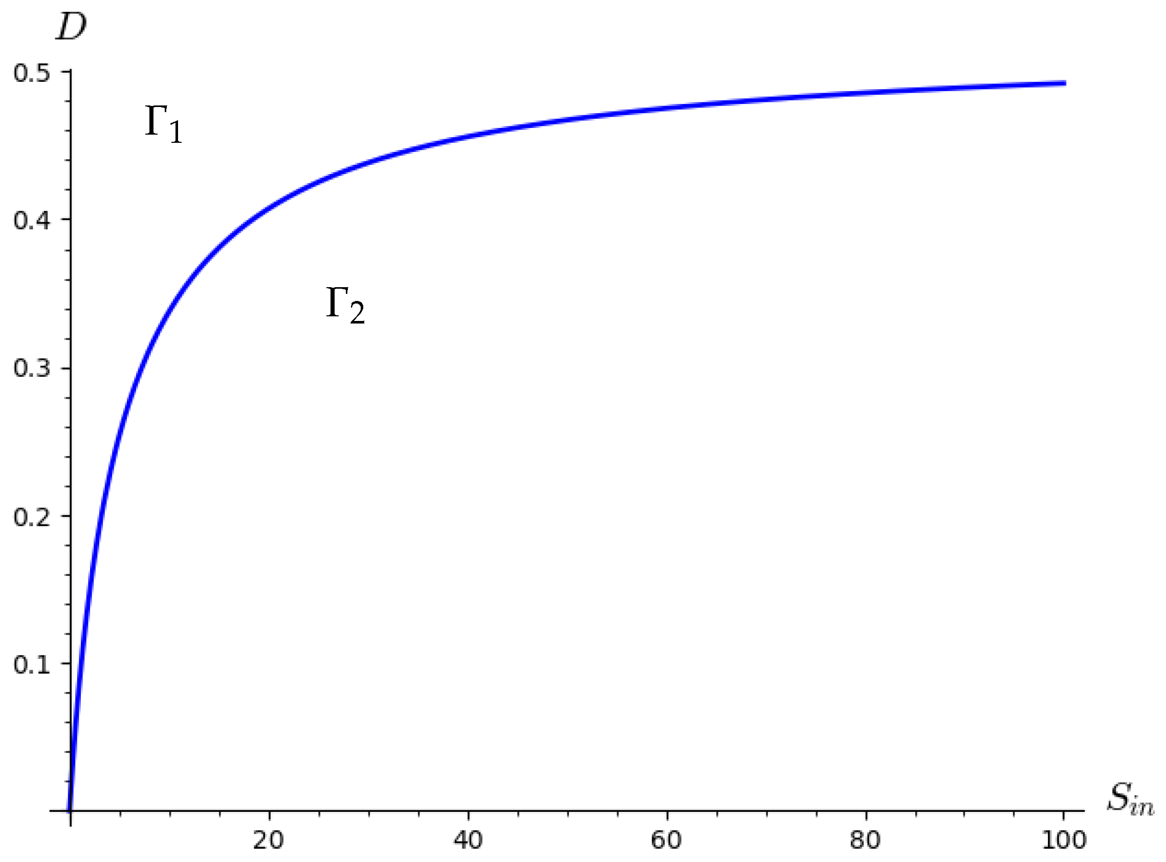
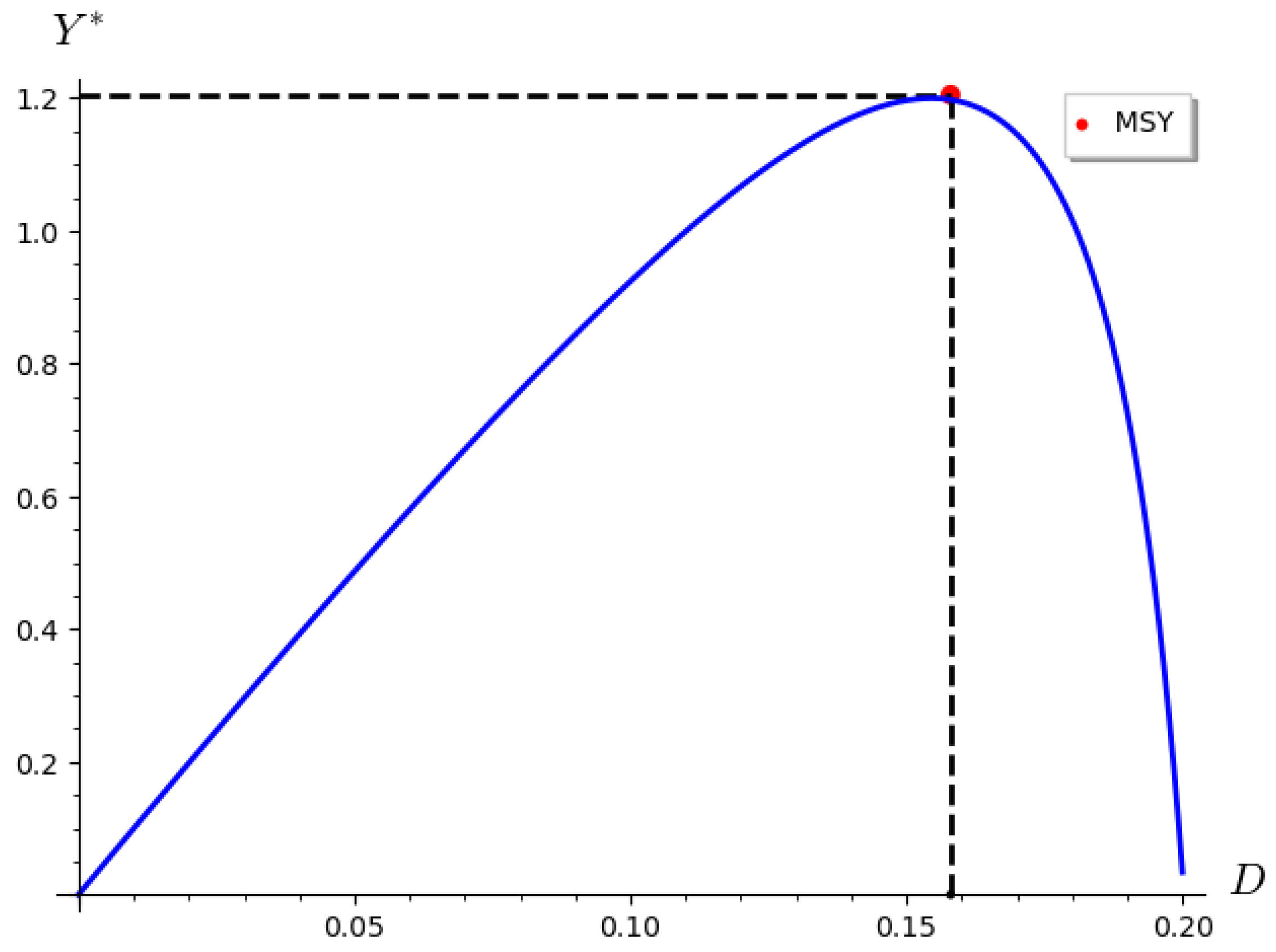
Some simulations are now shown to illustrate the results of the mathematical analysis of the aggregated model. Figure 4 shows the phase portrait (a) when the washout equilibrium is GAS and the positive equilibrium does not exist with parameter set D = 0.05 ; S i n = 10 ; μ = 0.03 ; u = 0.3 ; k = 0.5 , and (b) when the interior equilibrium is GAS and the washout equilibrium unstable with parameter set D = 0.2 ; S i n = 10 ; μ = 0.22 ; u = 0.3 ; k = 0.5 .  Figure 5 shows two regions in the parameter space ( S i n , D ) , region Γ 1 where the washout equilibrium is GAS and the positive equilibrium does not exist, region Γ 2 where the positive equilibrium is GAS and the washout equilibrium is unstable with parameter set μ = 0.4 , u = 0.3 , k = 5 . Figure 6 shows the yield at equilibrium with respect to the dilution rate for parameter set μ = 0.22 , u = 0.3 , k = 5 , s i n = 5 . It shows a maximum corresponding to the MSY.

3.3. Application to the Gradostat

By setting all parameters except D, the yield Y ( D ) = D x at equilibrium for the system of two coupled bioreactors reads as follows:
Y ( D ) = 2 D s i n D s
By substitution of s into the previous expression, the total yield reads:
Y ( D ) = 2 D s i n μ D k ( u 2 + ( 1 u ) 2 ) + k D 2 + D Δ 2 ( μ D ) u ( 1 u )
with Δ = [ μ k ( u 2 + ( 1 u ) 2 ) k D ] 2 + 4 D k 2 ( μ D ) u ( 1 u ) .
The excess yield at MSY of the reduced model is defined by the following expression: Δ Y M S Y = Y M S Y 2 Y M S Y u n where Y M S Y u n = μ s i n + k k 2 is the yield at MSY of an uncoupled bioreactor, using index u n for uncoupled. An excess yield in percentage is also defined as: % Δ Y M S Y = 100 Δ Y M S Y 2 Y M S Y u n .
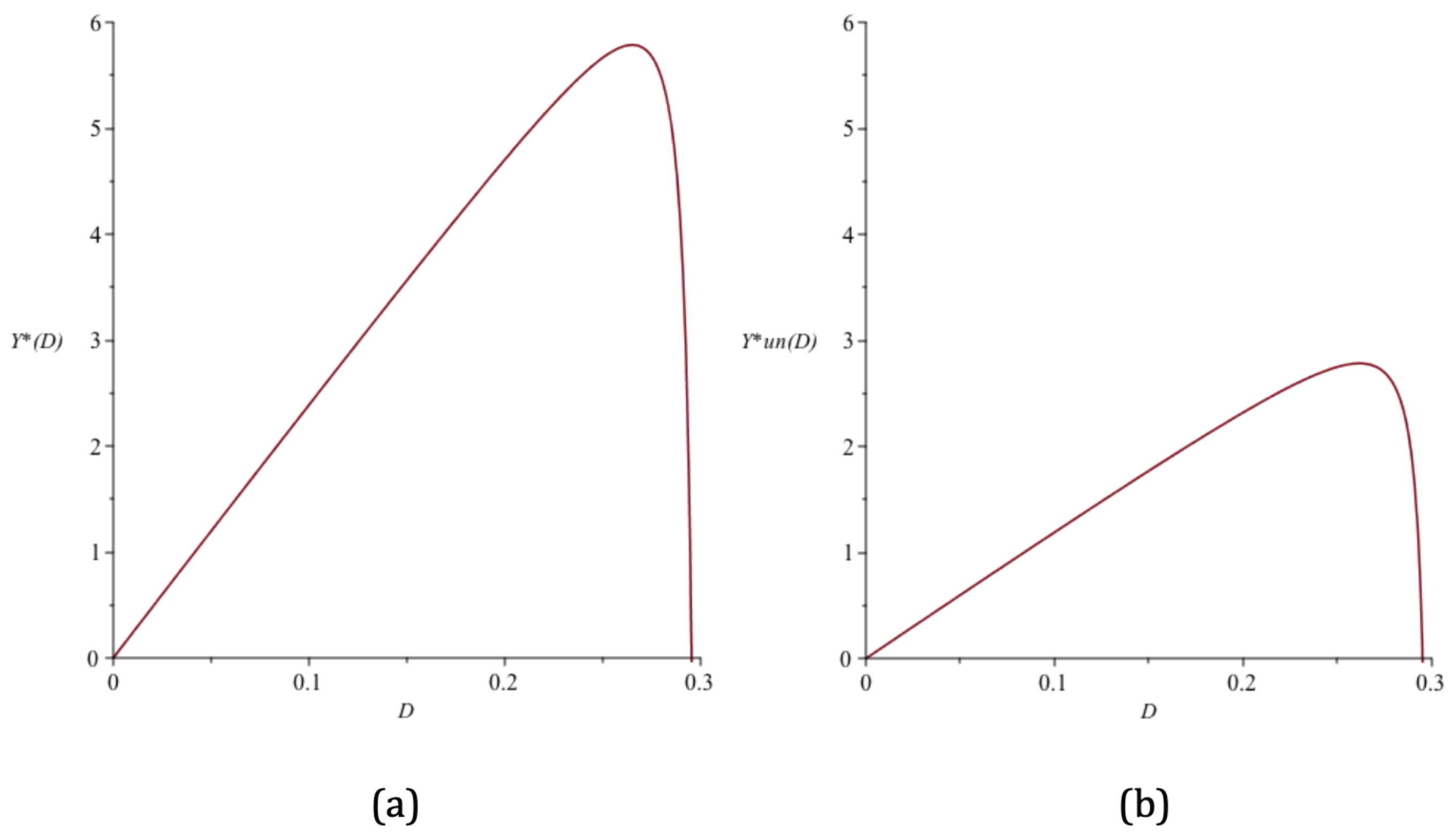
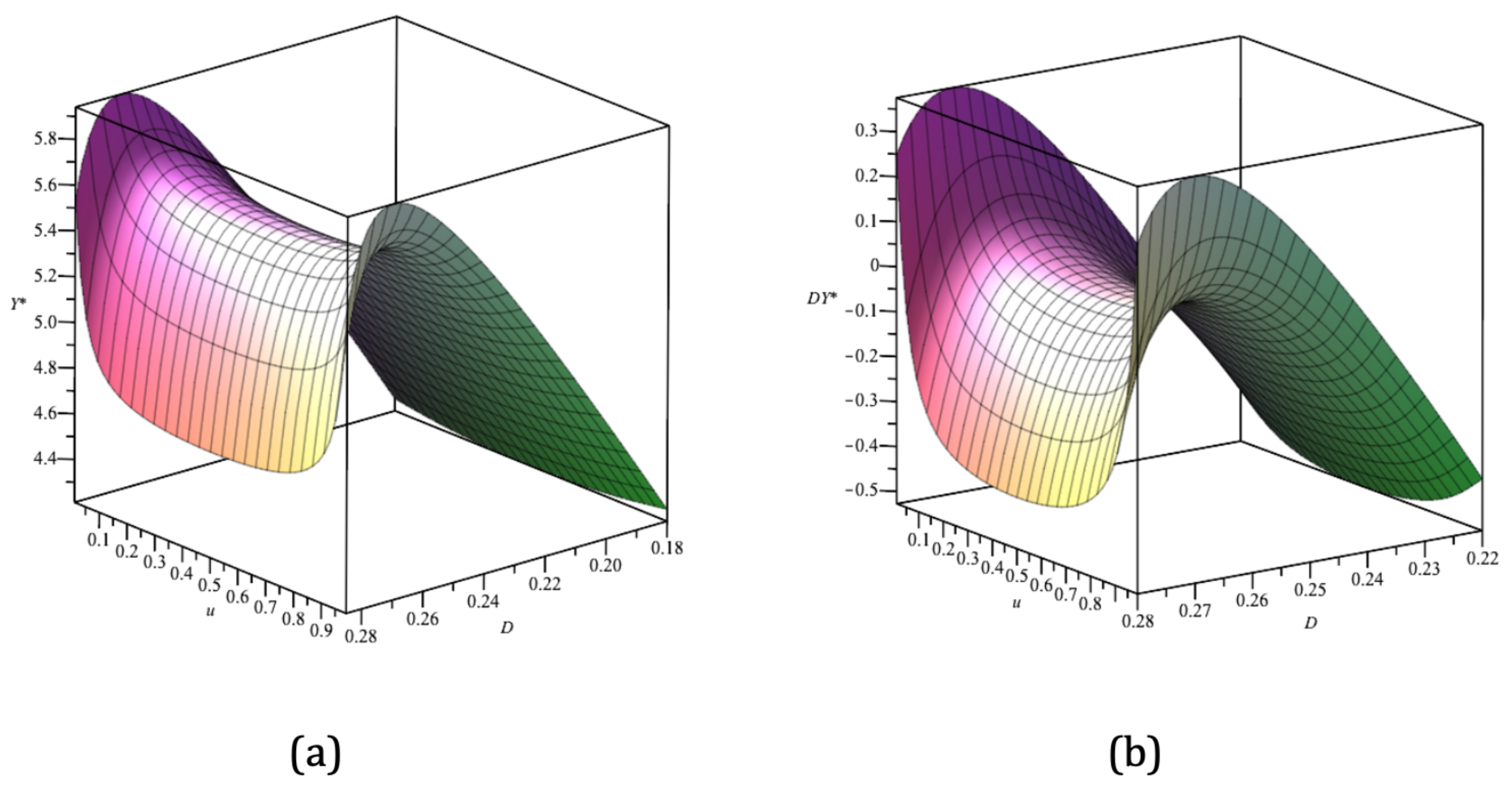
The values of the parameters correspond to the example of Zymomonas mobilis, which are used in a culture in a chemostat in a 60 m 3 fermenter, source [21]. Other parameters set: s i n = 12   g · L 1 , μ = 0.3   h 1 and k = 0.2   g · L 1 [21]. Figure 7a shows Yield Y ( D ) at equilibrium for the system of coupled bioreactors with respect to D and Figure 7b the Yield Y u n ( D ) at equilibrium for each uncoupled bioreactor. Each curve shows a maximum corresponding to the MSY, respectively at Y M S Y = 5.79   g · L 1 · h 1 for the system of coupled bioreactors and Y M S Y u n = 2.78   g · L 1 · h 1 for each uncoupled bioreactor. In that numerical example, for u = 0.95 , the yield at MSY for the gradostat is larger than the sum of the yields of uncoupled bioreactors. In this numerical example, Δ Y M S Y = 0.22   g · L 1 · h 1 , i.e., in percentage an increase in yield of 3.97 % . Excess productivity remains fairly limited in this example. However, chemostats are used for many cell cultures where higher yields could be obtained.
The two parameters that are under control are on the one hand the dilution rate D, and on the other hand the proportion of substrate and product u in reactor 1 by choosing the exchange rates m 1 and m 2 . Therefore, all parameters are fixed except u and D. Figure 8a shows the yield of the system of coupled bioreactors at equilibrium Y ( u , D ) as a function of u and D. Figure 8b shows the excess yield Δ Y M S Y ( u , D ) of the system of coupled bioreactors. As expected, for each value of u, the yield shows a maximum with respect to D associated with the corresponding MSY. The figures show that the yield and excess yield at MSY of the gradostat are higher when u is small or large, i.e., when one of the two tanks is almost empty of substrate and product.
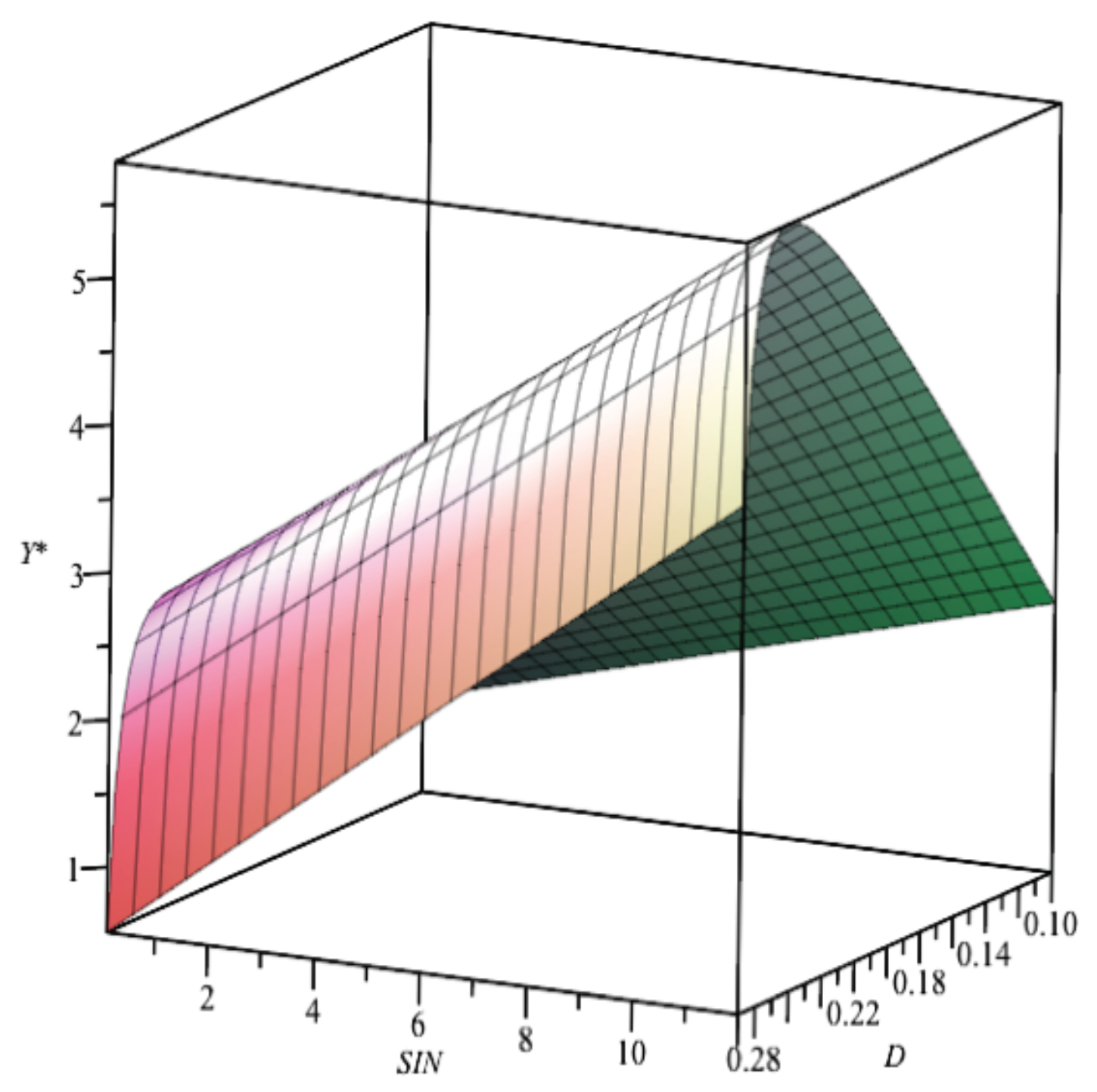
In general, the input substrate concentration cannot be increased beyond a certain value because some substances can be saturated. On the other hand, it can always be reduced by dilution. Thus, one can consider that the input substrate concentration can vary within a limited range. Figure 9 shows Yield Y ( s i n , D ) at equilibrium for the system of coupled chemostats with respect to s i n and D. It shows that for each s i n value, there exists an optimal dilution rate D M S Y . As expected, the yield at MSY increases as s i n increases. As a consequence, the key parameters to get an optimal yield are really u, the proportion of substrate and products in the first chemostat at the fast equilibrium and the dilution rate D.

3.4. Application to Fish Farming

In the context of fish farming, by analogy, the substrate can be seen as the prey and the product as a predator. The two chemostats correspond to rearing ponds connected by channels allowing prey and predatory fish to pass from one pond to another. In addition, depending on the species, the feeding rates as well as the growth rates of the species can vary over fairly wide ranges, source [24]. Accordingly, in the following example, the next parameter set is considered: μ = 8.5 , k = 2.5 , s i n = 0.5 . The model presented remains very simplified in terms of aquaculture. However, it could present some characteristics of fish farming. In fact, in breeding ponds, the prey used as food for predators are quickly consumed, and the growth of the prey that takes place outside the system can be neglected. Predators grow slowly in ponds, and the natural mortality of the predator, which is reared in a disease-free, controlled environment and is removed when it reaches a sufficient size, can usually be overlooked. In addition, the Monod function corresponds to the classical Holling type II functional response in prey–predator models.
Modern aquaculture seeks to replace flour with coproducts from the fishing industry [25,26]. Here, the introduction of small fish into the ponds, which could serve as prey or even algae, is considered. s i n corresponds to the concentration of food (such as small fish) that serve as prey for predator fish in breeding ponds. In this context, the dilution rate of the slow model amounts to the fishing effort. Here, for the sake of simplicity, the growth of farmed fish takes place over the long term. In the case of a cage at sea where fish are reared, the constancy of the volume is ensured. In addition, the food is consumed quickly and somehow does not have time to get out of the cages. In the case of rearing ponds, maintaining the constant volume of each pond would require fast entry/exit flows to compensate for the flows between the two ponds. It could be possible by using screens to extract seawater (or fresh water) from the ponds while keeping predatory fish and their food (prey fish, algae...) inside the ponds. In this simplified case, the fast input and output flows operate in a loop, the water withdrawn from the basin that fills up is reinjected into the basin, which is emptied to maintain a constant volume in each basin.
Figure 10a shows the yield of the system of coupled rearing ponds at equilibrium Y ( u , D ) as a function of u and D. Figure 10b shows the excess yield Δ Y M S Y ( u , D ) of the system of coupled rearing ponds. As expected, for each value of u, the yield shows a maximum with respect to D associated with the corresponding MSY. The figures still show that the yield and excess yield at MSY of the system of coupled rearing ponds are higher when u is small or large, i.e., when one of the two basins is almost empty of fish.
Table 1 shows results for the same set of parameters and for different values of the proportion of food concentration and fish u in pond 1 ranging from 0.01 to 0.50 insofar as the curve is symmetric with respect to u = 0.5 . The table shows that the increase in the yield is almost everywhere positive. Furthermore, Table 1 shows for example that with a value of u = 0.05 , one benefits from an excess of yield at the MSY of about 68 % , which is a huge value. This means that it is profitable to couple the two rearing ponds with fish exchanges while maintaining a strong asymmetry between the two ponds: one at 95 % , and the other at 5 % of fish. Table 1 shows that even for rather symmetrical partitions of fish between the two bioreactors, for example u = 0.35 , a significant increase in excess yield is still obtained, i.e., in percentage 7.5 % , which is not negligible.
Finally, the coupling of the two basins remains profitable in a wide range of values of proportion of u, and it allows one to find the feeding rate that optimizes the total yield for any u.

4. Concluding Remarks and Perspectives

This work aimed at generalizing the notion of Maximum Sustainable Yield (MSY) to the simple case of the classical chemostat with the Monod function, by searching for the dilution rate that optimizes the synthesis of the product at equilibrium. This result was already known, but it was extended to the case of the coupling of two bioreactors connected by exchanges of substrate and product at the fast timescale. The study showed that the product excess synthesis between the system of coupled reactors and the two uncoupled ones is greater when a large asymmetry between the two coupled bioreactors is maintained.
The work presented remains very theoretical and quite far from immediate applications. Indeed, regarding the gradostat, a very simplified case where efficient substrate filtration is possible was considered. The general case with incomplete filtering would require determining the input and output flows (at the fast time scale) of the bioreactors such as to maintain constant volumes, as well as the substrate concentrations at a constant level. The technical aspects could prove difficult in practice. The study of the general case and its applicability seem an interesting subject that could be tackled in a later work in collaboration with specialists of bioreactors.
In this work, a single dilution rate was taken into account. As a perspective, the case with two different dilution rates for each bioreactor could be examined. The extension of the study to the case of a larger number (greater than two) of bioreactors coupled in the “gradostat” would also be of some interest. The study of the effect of the number of coupled bioreactors on the overall product synthesis at MSY would need more attention. Another perspective would consist of studying the case of two coupled bioreactors with one substrate and two products, and researching the conditions of coexistence of the “competitors” as well as the optimal conditions of global products synthesis.
Regarding the application to fish farming, it would be necessary to consider a given commercial species and adapt the model to real farming conditions in two sites. It appears difficult to have values concerning the feeding parameters of the fish as well as those concerning their growth. Collaboration with specialists in aquaculture should make it possible to seek practical application of the theoretical results obtained.

Author Contributions

The authors (P.A. and A.M.) contributed equally to this work. All authors have read and agreed to the published version of the manuscript.

Funding

This research received no external funding.

Institutional Review Board Statement

Not applicable.

Informed Consent Statement

Not applicable.

Data Availability Statement

Not applicable.

Conflicts of Interest

The authors declare no conflict of interest.

Appendix A

Consider the following system of retarded functional differential equations
X ( t ) = F ( t , X t ) , X t = X ( t + θ ) ,
where
X ( t 0 ) = X ( t 0 + θ ) = ϕ ( θ ) , < θ 0
is the initial condition. Here, the function ϕ is chosen from the space of all bounded, continuous functions on ( , O ] , denoted by BC ( , O ] with appropriate norm. X ( t ) = F ( t 0 , ϕ ) is assumed.
The following theorem is due to Burton [23], which provides conditions under which the solutions of (A1) are bounded.
Theorem A1
(Burton’s Theorem). Let V ( t , x ( . ) ) be continuous, locally Lipschitz in x, uniformly positive definite and strongly decrescent:
W ( t , x ( t ) ) V ( t , x ( t ) ) Q ( t , x ( t ) ) + m sup α ( t ) s t W ( s , x ( s ) )
for a continuous function α ( t ) α and m < 1 . Suppose there is a positive number U ˜ with V ( A1 ) 0 if Q ( t , x ( t ) ) U ˜ . Then solutions of (A1) are uniformly bounded.

References

  1. Iwasa, Y.; Levin, S.; Andreasen, V. Aggregation in model ecosystems II. Approximate aggregation. Math. Med. Biol. 1989, 6, 1–23. [Google Scholar] [CrossRef]
  2. Auger, P.; Poggiale, J.-C.; Sanchez, E. A review on spatial aggregation methods involving several time scales. Ecol. Comp. 2012, 10, 12–25. [Google Scholar] [CrossRef]
  3. Auger, P.; Bravo de la Parra, R.; Poggiale, J.C.; Sánchez, E.; Nguyen Huu, T. Aggregation of variables and applications to population dynamics. In Structured Population Models in Biology and Epidemiology; Lecture Notes in Mathematics; Magal, P., Ruan, S., Eds.; Springer: Berlin/Heidelberg, Germany, 2008; Volume 1936, pp. 209–263. [Google Scholar]
  4. Auger, P.; Bravo de la Parra, R.; Poggiale, J.C.; Sánchez, E.; Sanz, E. Aggregation methods in dynamical systems and applications in population and community dynamics. Phys. Life Rev. 2008, 5, 79–105. [Google Scholar] [CrossRef] [Green Version]
  5. Marvá, M.; Bravo de la Parra, R.; Poggiale, J.C. Reduction of slow-fast asymptotically autonomous systems with applications to gradostat models. Ecol. Complex. 2013, 14, 75–84. [Google Scholar] [CrossRef]
  6. Fenichel, N. Persistence and smoothness of invariant manifolds for flows. Indiana Univ. Math. J. 1971, 21, 193–226. [Google Scholar] [CrossRef]
  7. Marvá, M.; Poggiale, J.-C.; Bravo de la Parra, R. Reduction of slow-fast periodic systems: Fast migrations in a predator–prey community. Math. Model. Methods Appl. Sci. 2012, 22, 1250025. [Google Scholar] [CrossRef] [Green Version]
  8. Schaefer, M.B. Some aspects of the dynamics of populations important to the management of commercial marine fisheries. Bull. Inter-Am. Trop. Tuna Comm. 1954, 1, 25–56. [Google Scholar]
  9. Clark, C.W. Mathematical Bioeconomis. In The Optimal Management of Renewable Resources, 2nd ed.; John Wiley & Sons, Inc.: New York, NY, USA, 1990. [Google Scholar]
  10. Murray, J.D. Mathematical Biology I. An Introduction; Springer: New York, NY, USA, 2002. [Google Scholar]
  11. Legovic, T.; Gecek, S. Impact of maximum sustainable yield on independent populations. Ecol. Model. 2010, 221, 2108–2111. [Google Scholar] [CrossRef]
  12. Ghosh, B.; Kar, T. Maximum sustainable yield and species extinction in a prey–predator system: Some new results. J. Biol. Phys. 2013, 39, 453–467. [Google Scholar] [CrossRef] [PubMed] [Green Version]
  13. Kar, T.K.; Ghosh, B. Impacts of maximum sustainable yield policy to prey–predator systems. Ecol. Model. 2013, 250, 134–142. [Google Scholar] [CrossRef]
  14. Legovic, T.; Klanjscek, J.; Gecek, S. Maximum sustainable yields and species extinction in ecosystems. Ecol. Model. 2011, 221, 1569–1574. [Google Scholar] [CrossRef]
  15. Legovic, T.; Gecek, S. Impact of maximum sustainable yield on mutualistic communities. Ecol. Model. 2012, 230, 63–72. [Google Scholar] [CrossRef]
  16. Harmand, J.; Lobry, C.; Rapaport, A.; Sari, T. The Chemostat: Mathematical Theory of Microorganisms Culture; ISTE Ltd. and John Wiley: Hoboken, NJ, USA, 2017. [Google Scholar]
  17. Smith, H.L.; Waltman, O. The Theory of the Chemostat: Dynamics of Microbial Competition; Cambridge University Press: Cambridge, UK, 1995. [Google Scholar]
  18. Dali-Youcef, M.; Rapaport, A.; Sari, T. Study of performance criteria of serial configuration of two chemostats. Math. Biosci. Eng. 2021, 17, 6278–6309. [Google Scholar] [CrossRef] [PubMed]
  19. Caraballo, T.; Lopez-de-laCruz, J.; Rapaport, A. Study of the dynamics of two chemostats connected by Fickian diffusion with bounded random fluctuations. Stoch. Dyn. 2021, 2240002. [Google Scholar] [CrossRef]
  20. Pavlou, S. Microbial competition in bioreactors. CICEQ 2006, 12, 71–81. [Google Scholar] [CrossRef]
  21. Doran, P. Bioprocess Engineering Principles, 2nd ed.; Elsevier: Heidelberg, Germany, 2013. [Google Scholar]
  22. Tikhonov, A.N. Systems of differential equations containing small parameters in the derivatives. Mat. Sb. 1952, 70, 575–586. [Google Scholar]
  23. Burton, T.A. Volterra Integral and Differential Equations, 2nd ed.Mathematics in Sciences & Engineering; Elsevier: Amsterdam, The Netherlands, 2005. [Google Scholar]
  24. Campbell, D. United Nations Development Programme Food and Agriculture Organization of the United Nations Nigerian Institute for Oceanography and Marine Research Project Raf/82/009: A Review of the Biology and Culture of Tilapia guineensis. 1987. Available online: http://www.fao.org/3/ac165e/ac165e00.htm (accessed on 11 January 2021).
  25. CIPA Report. Available online: https://www.poisson-aquaculture.fr (accessed on 9 January 2021).
  26. Johnson, M.P. Farm Production Diversity in Aquaculture Has Been Overlooked as a Contributor to Sustainability. Front. Sustain. Food Syst. 2021, 5, 1–8. [Google Scholar] [CrossRef]
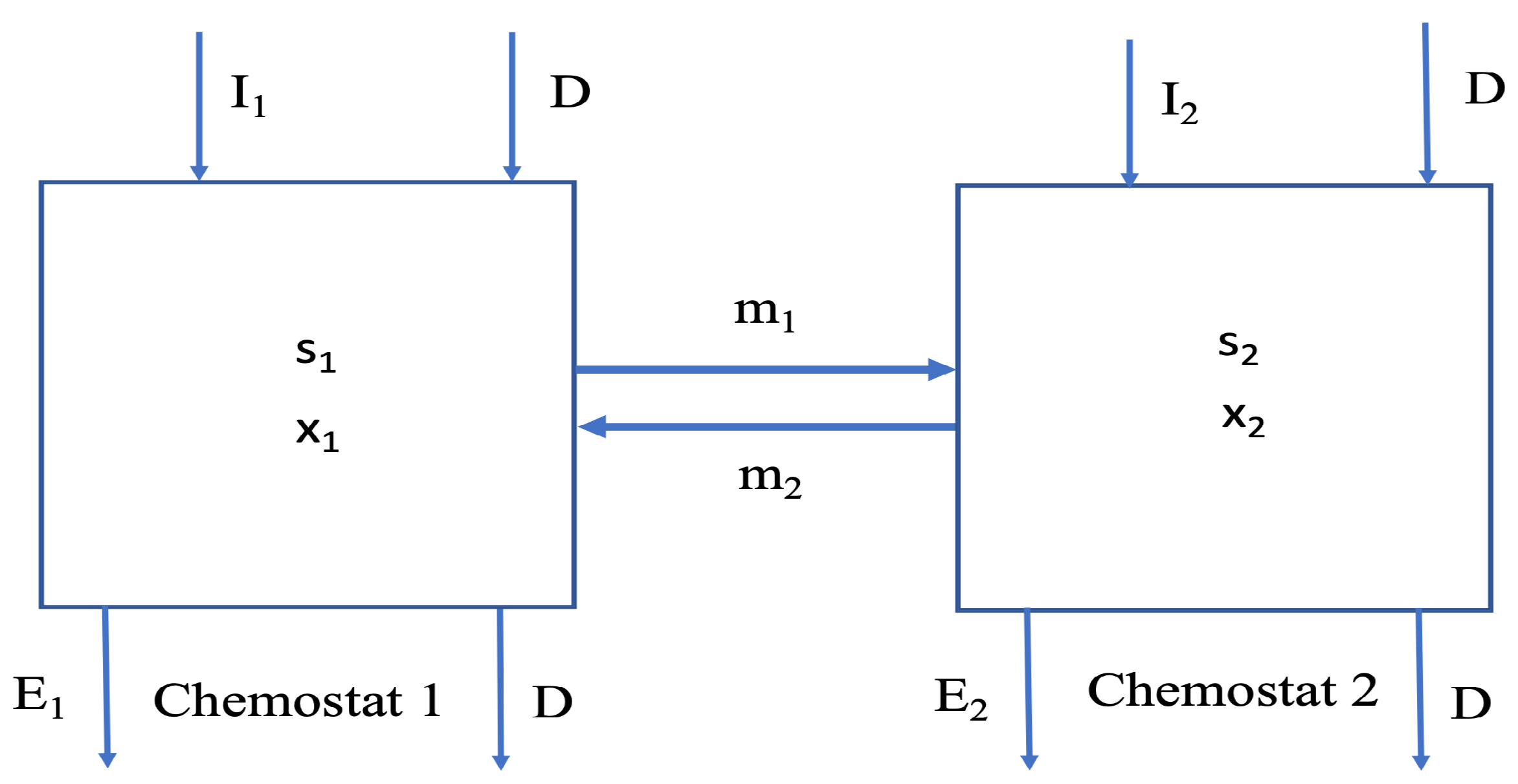
Figure 1. System of two connected bioreactors with fast exchanges.
Mathematics 10 00555 g001
Figure 2. Output product flux at equilibrium with respect to dilution rate. Parameters set: s i n = 2 , μ m a x = 5 and k = 5 . In this case, s = 0.88 and x = 1.12 . Yield Y ( D ) shows a maximum.
Mathematics 10 00555 g002
Figure 3. Comparison of complete (blue) and aggregated (red) solutions. (a) m 1 = 0.3 , m 2 = 0.7 and ϵ = 0.1 (b) m 1 = 3 , m 2 = 7 and ϵ = 1 . Parameters set: s i n = 0.5 , u = 0.7 , μ = 8.5 and k = 2.5 . Initial conditions for complete model are s 1 ( 0 ) = s 2 ( 0 ) = 0.2 , x 1 ( 0 ) = x 2 ( 0 ) = 0.1 , and for aggregated model s ( 0 ) = 0.4 , x ( 0 ) = 0.2 .
Mathematics 10 00555 g003
Figure 4. Phase portrait of aggregated model. (a) Parameter set: D = 0.05 , S i n = 10 ; μ = 0.03 ; u = 0.3 ; k = 0.5 . (b) Parameter set: D : 0.2 , S i n = 10 ; μ = 0.22 ; u = 0.3 ; k = 0.5 . .
Mathematics 10 00555 g004
Figure 5. Parameter set: μ = 0.4 , u = 0.3 , k = 5 , graph of function D = f ( S i n ) . Region Γ 1 , where washout equilibrium is GAS and positive equilibrium does not exist. Region Γ 2 , where positive equilibrium is GAS and washout equilibrium is unstable.
Mathematics 10 00555 g005
Figure 6. Parameter set: μ = 0.22 , u = 0.3 , k = 5 , s i n = 5 , graph of function Y = f ( D ) .
Mathematics 10 00555 g006
Figure 7. (a) Yield Y ( D ) at equilibrium for the system of coupled chemostats with respect to D. (b) Yield Y u n ( D ) at equilibrium for each uncoupled chemostat. Parameters set: μ = 0.3   h 1 , k = 0.2   g · L 1 , s i n = 12   g · L 1 and u = 0.95 .
Mathematics 10 00555 g007
Figure 8. (a) Yield Y ( u , D ) at equilibrium for the system of coupled chemostats with respect to u and D. (b) Excess Yield Δ Y ( u , D ) at equilibrium for the system of coupled chemostats with respect to u and D. Parameters set: μ = 0.3   h 1 , k = 0.2   g · L 1 and s i n = 12   g · L 1 .
Mathematics 10 00555 g008
Figure 9. Yield Y ( s i n , D ) at equilibrium for system of coupled chemostats with respect to s i n and D. Parameters set: μ = 0.3   h 1 , k = 0.2   g · L 1 and s i n = 12   g · L 1 .
Mathematics 10 00555 g009
Figure 10. (a) Yield Y ( u , D ) at equilibrium for system of coupled rearing basins with respect to u and D. (b) Excess Yield Δ Y ( u , D ) at equilibrium for system of coupled rearing basins with respect to u and D. Parameters set: s i n = 0.5 , μ = 8.5 and k = 2.5 .
Mathematics 10 00555 g010
Table 1. Table of yields at MSY: Y M S Y , Y M S Y u n , Δ Y M S Y , % Δ Y M S Y with respect to proportion of fish in pond 1, with parameter set: μ = 8.5 , k = 2.5 , s i n = 0.5 .
u Y M S Y 2 Y M S Y u n Δ Y M S Y % Δ Y M S Y
0.010.700.390.3180.1%
0.050.650.390.2668.1%
0.100.590.390.2154.7%
0.150.540.390.1641.1%
0.200.500.390.1230.1%
0.250.470.390.0820.9%
0.300.440.390.0513.4%
0.350.420.390.037.5%
0.400.400.390.0133.3%
0.450.390.390.0030.8%
0.500.380.39negativeundefined
Publisher’s Note: MDPI stays neutral with regard to jurisdictional claims in published maps and institutional affiliations.