Article

Novel Generalized Proportional Fractional Integral Inequalities on Probabilistic Random Variables and Their Applications

by
Weerawat Sudsutad
1,†,
Nantapat Jarasthitikulchai
2,*,†,
Chatthai Thaiprayoon
3,4,†,
Jutarat Kongson
3,4,*,† and
Jehad Alzabut
5,6,†
1
Department of Statistics, Faculty of Science, Ramkhamhaeng University, Bangkok 10240, Thailand
2
Department of General Education, Faculty of Science and Health Technology, Navamindradhiraj University, Bangkok 10300, Thailand
3
Department of Mathematics, Faculty of Science, Burapha University, Chonburi 20131, Thailand
4
Center of Excellence in Mathematics, CHE, Sri Ayutthaya Rd., Bangkok 10400, Thailand
5
Department of Mathematics and Sciences, Prince Sultan University, Riyadh 11586, Saudi Arabia
6
Department of Industrial Engineering, OSTİM Technical University, Ankara 06374, Turkey
*
Authors to whom correspondence should be addressed.
These authors contributed equally to this work.
Mathematics 2022, 10(4), 573; https://doi.org/10.3390/math10040573
Submission received: 29 November 2021 / Revised: 27 January 2022 / Accepted: 10 February 2022 / Published: 12 February 2022
(This article belongs to the Special Issue Mathematical Inequalities with Applications)

Abstract

:
This study investigates a variety of novel estimations involving the expectation, variance, and moment functions of continuous random variables by applying a generalized proportional fractional integral operator. Additionally, a continuous random variable with a probability density function is presented in context of the proportional Riemann–Liouville fractional integral operator. We establish some interesting results of the proportional fractional expectation, variance, and moment functions. In addition, constructive examples are provided to support our conclusions. Meanwhile, we discuss a few specific examples that may be extrapolated from our primary results.

1. Introduction

Integral inequality is the motivating force behind the modern mathematical analysis perspective. It has been used in a variety of fields, including probability theory and statistical problems, mathematics, physics, and applied sciences; see [1,2]. The integral inequality theory has developed into a vibrant and self-contained sector of research. Fractional calculus has represented an essential role in the study of integral inequality using various forms of fractional integral operators. Several researchers have produced widely disparate conclusions concerning fractional integral inequalities and their applications; see some works [3,4,5,6,7,8,9,10,11,12,13,14,15,16,17,18,19,20,21,22,23,24] and references cited therein. Integral inequality has also been employed in probability theory, and it continues to pique researchers’ curiosity.
Fractional calculus (FC) has been widely studied recently over the past decades (beginning in 1695) in fields of applied sciences and engineering. Fractional calculus deals with fractional-order (non-integer-order) differential and integral operators, which establish phenomenon modeling that is increasingly realistic in real-world problems. Moreover, it has properly specified the term “memory”, particularly in mathematics, physics, chemistry, biology, mechanics, electricity, finance, economics, and control theory. However, various types of fractional integral operators have been used in research works that mostly focus on the Riemann–Liouville (RL), Caputo, Hadamard, Katugampola, generalized conformable, and proportional types; see [25,26,27,28,29,30,31].
A probability density function is often used in statistical analysis to represent the relationship between unknown parameters and measures conducted to understand more about them. When there is enough data collected to investigate a solution for the parameters, a powerful estimation technique needs to be used, such as FC, which is an optimal tool under a wide range of criteria. The distribution function and density functions can be used to obtain a detailed description of the probability distribution for a given random variable. To gain a thorough explanation of the probability distribution for a random variable, distribution functions and density functions can be engaged. Surprisingly, they do not allow us to compare two different distributions. In designation comparisons, the random variables that depict the allocation, in particular, under realistic assumptions are useful. As we know, the expectation and variance functions may be calculated using the probability function. However, there are applications where the exact forms of probability distributions are unknown or mathematically difficult, preventing the estimation of the moments—for example, an application in insurance involving the insurer’s payout on a given agreement or group of agreements that follows a combination or hybrid probability distribution. This challenge drives academics to seek alternate estimates for a probability distribution’s expectations and variances. Some novel estimates for the expectation and variance of random variables were investigated using inequality techniques in [32,33].
Several researchers have recently investigated a variety of fractional applications for a continuous random variable ( C . R . V ) with a probability density function ( P . D . F ). For example, Dahmani [34] applied the RL-fractional integral operator to analyze integral inequality results for the fractional expectation ( F . E ) and fractional variance ( F . V ) functions of the C . R . V in 2014. After that, in 2015, Akkurt and co-workers [35] established several extensions of the integral inequality results in [34] by using the Katugampola fractional integral operator. In 2016, Some applications of the RL-fractional integral operator for the C . R . V were presented by Dahmani [36]. In addition, he explored and rectified some integral inequalities via the F . E and F . V functions, as well as several corollaries in [34]. Additionally, in [37,38], the authors provided novel W-weighted ideas for the C . R . V with an RL-fractional integral operator with its applications in 2017. In 2019, the Hadamard fractional integral operator was used by Khellaf and co-workers [39] to construct several novel integral inequalities of the F . E and F . V functions of the C . R . V . In 2020, Chen and co-workers [40] analyzed numerous novel inequalities in the context of a generalized RL-fractional integral operator with respect to another function via the C . R . V . The results are the generalizations and enhancements of the previously published papers in [41,42,43,44,45,46,47,48,49,50] and references therein.
Motivated by the aforesaid utilization above and the series of papers that were presented, the aim of this work is to present novel ideas about generalized proportional fractional random variables. We establish some novel estimates for the C . R . V by utilizing the generalized proportional fractional integral operator with respect to another function. The novel proportional F . E and proportional F . V results are also presented. As special instances, several classical integral inequality findings can be derived. Finally, the conclusion of this paper is presented in the last section.

2. Preliminaries

The generalized proportional fractional integral operators, definitions, and introductory facts are introduced in this section, which will be used throughout this work.
Definition 1.
([25]). Assume that u [ 1 , ) , v 0 and a < b . Hence, h ( t ) is called in L u , v ( a , b ) -space if
h L u , v ( a , b ) = a b | h ( t ) | u t v d t 1 / u < .
If v = 0 , we have
L u , 0 ( a , b ) = L u ( a , b ) = h : h L u ( a , b ) = a b | h ( t ) | u d t 1 / u < .
Definition 2.
([14]). Let h L 1 [ 0 , ) . Assume that ϕ C 1 ( [ a , b ] ) and ϕ > 0 . Hence, X ϕ p ( 0 , ) is the space of all the real-valued Lebesgue measureable functions h, defined on R + { 0 } so that
h X ϕ u ( 0 , ) = 0 | h ( t ) | u ϕ ( t ) d t 1 / u < , u [ 1 , ) .
If u = , h X ϕ ( 0 , ) is given by
h X ϕ ( 0 , ) = e s s sup 0 t < ϕ ( t ) h ( t ) .
In particular, if ϕ ( t ) = t , then X ϕ u ( 0 , ) coincides with a L u [ 0 , ) -space with u [ 1 , ) ; if ϕ ( t ) = t v + 1 / ( v + 1 ) , u [ 1 , ) , v 0 , then X ϕ u ( 0 , ) reduces to a L u , v [ 0 , ) -space.
Definition 3.
([30,31]). Let α C , R e ( α ) > 0 , ρ ( 0 , 1 ] , ϕ C 1 ( [ a , b ] ) , ϕ > 0 . The proportional fractional integral of order α of h L 1 ( [ a , b ] ) with respect to ϕ is given by
ρ I a + α , ϕ [ h ( t ) ] = 1 ρ α Γ ( α ) a t ρ G ϕ α ( t , s ) h ( s ) ϕ ( s ) d s ,
where Γ ( α ) = 0 s α 1 e s d s , s > 0 and
ρ G ϕ α ( x , y ) = e ρ 1 ρ ϕ ( x ) ϕ ( y ) ϕ ( x ) ϕ ( y ) α 1 .
We provide the following semi-group property:
ρ I a + α , ϕ ρ I a + β , ϕ [ h ( t ) ] = ρ I a + β , ϕ ρ I a + α , ϕ [ h ( t ) ] = ρ I a + α + β , ϕ [ h ( t ) ] , α , β 0 ,
and
ρ I a + α , ϕ ρ G ϕ β ( t , a ) = Γ ( β ) ρ α Γ ( β + α ) ρ G ϕ β + α ( t , a ) , α 0 , β > 0 .
Remark 1.
It is easy to see that if we set ρ = 1 in Definition 3, we have the following:
( A 1 )
The RL-fractional integral operator defined as in [25] with ϕ ( t ) = t ;
( A 2 )
The Hadamard fractional integral operator defined as in [25] with ϕ ( t ) = ln t ;
( A 3 )
The Katugampola fractional integral operator defined as in [26] with ϕ ( t ) = t μ / μ for μ > 0 ;
( A 4 )
The conformable fractional integral operator defined as in [27] with ϕ ( t ) = ( t a ) μ / μ for μ > 0 ;
( A 5 )
The generalized conformable fractional integral operator defined as in [28] with ϕ ( t ) = t μ + ϕ / ( μ + ϕ ) .
Firstly, we give the proportional F . E function of X .
Definition 4.
Assume that X is a random variable with a positive P . D . F h defined on ( a , b ) , and ϕ ( t ) is an increasing and positive function defined on ( a , b ) . Then, the proportional F . E function of order α 0 is given by
ρ E X , α ( t ) = ρ I a + α , ϕ e ρ 1 ρ ϕ ( t ) ϕ ( t ) h ( t ) = 1 ρ α Γ ( α ) a t ρ G ϕ α ( t , s ) e ρ 1 ρ ϕ ( s ) ϕ ( s ) h ( s ) ϕ ( s ) d s ,
where the proportional expectation is given by
ρ E ( X ) = ρ E X , 1 ( b ) = 1 ρ e ρ 1 ρ ϕ ( b ) a b ϕ ( s ) h ( s ) ϕ ( s ) d s .
Next, we give the proportional F . E function of X ρ E ( X ) .
Definition 5.
Assume that ϕ ( t ) is an increasing and positive function defined on ( a , b ] . Then the proportional F . E function of order α 0 for a random variable X ρ E ( X ) is given by
ρ E X ρ E ( X ) , α ( t ) = 1 ρ α Γ ( α ) a t ρ G ϕ α ( t , s ) e ρ 1 ρ ϕ ( s ) ϕ ( s ) ρ E ( X ) h ( s ) ϕ ( s ) d s ,
where h : [ a , b ] R + is the P . D . F . of X .
If t = b , then we obtain the following definition.
Definition 6.
Assume that ϕ ( t ) is an increasing and positive function defined on ( a , b ) . Then ρ E X , α ( t ) of order α 0 for a random variable X with a positive P . D . F f defined on ( a , b ) is given by
ρ E X , α ( b ) = 1 ρ α Γ ( α ) a b ρ G ϕ α ( b , s ) e ρ 1 ρ ϕ ( s ) ϕ ( s ) h ( s ) ϕ ( s ) d s .
For the proportional F . V function of X , we have the following two definitions.
Definition 7.
Assume that ϕ ( t ) is an increasing and positive function defined on ( a , b ) . Then, the proportional F . V function ρ σ X , α 2 ( t ) of order α 0 for a random variable X with a positive P . D . F h defined on ( a , b ) is given by
ρ σ X , α 2 ( t ) = ρ I a + α , ϕ e ρ 1 ρ ϕ ( t ) ϕ ( t ) ρ E ( X ) 2 h ( t ) = 1 ρ α Γ ( α ) a t ρ G ϕ α ( t , s ) e ρ 1 ρ ϕ ( s ) ϕ ( s ) ρ E ( X ) 2 h ( s ) ϕ ( s ) d s .
If t = b , then we get the following definition.
Definition 8.
Assume that ϕ ( t ) is an increasing and positive function defined on ( a , b ) . Then, the generalized proportional F . V function ρ σ X , α 2 ( t ) of order α 0 for a random variable X with a positive P . D . F   h : ( a , b ) R + is given by
ρ σ X , α 2 ( b ) = 1 ρ α Γ ( α ) a b ρ G ϕ α ( b , s ) e ρ 1 ρ ϕ ( s ) ϕ ( s ) ρ E ( X ) 2 h ( s ) ϕ ( s ) d s .
Definition 9.
Assume that X is a random variable with a positive P . D . F h defined on ( a , b ) and ϕ ( t ) is an increasing and positive function defined on ( a , b ) . Then the proportional fractional moment ( F . M ) function of order ( r , α ) with α 0 , r > 0 is given by
ρ M X r , α ( t ) = ρ I a + α , ϕ e ρ 1 ρ ϕ ( t ) ϕ ( t ) r h ( t ) = 1 ρ α Γ ( α ) a t ρ G ϕ α ( t , s ) e ρ 1 ρ ϕ ( s ) ϕ ( s ) r h ( s ) ϕ ( s ) d s .
Remark 2.
It is easy to see that:
( A 1 )
If we input ρ = α = 1 , and ϕ ( t ) = t in Definition 4, it yields that the classical expectation E ( X ) = a b s h ( s ) d s ;
( A 2 )
If we input ρ = α = 1 , and ϕ ( t ) = t in Definition 7, it yields that the classical variance σ 2 = a b s E ( X ) 2 h ( s ) d s ;
( A 3 )
If we input ρ = α = 1 , and ϕ ( t ) = t in Definition 9, it yields that the classical moment of order r: M r = a b s r h ( s ) d s ;
( A 4 )
If we input ρ = 1 , and ϕ ( t ) = t in Definitions 4–9, it yields Definitions 2.2 2.6 in [34] and Definition 2.3 in [36];
( A 5 )
If we input ρ = 1 in Definitions 4–8, it yields Definitions 2.5 2.9 in [40].
( A 6 )
For α > 0 , the P . D . F h satisfies
ρ I a + α , ϕ [ h ( b ) ] = ρ G ϕ α ( b , a ) ρ α Γ ( α ) = e ρ 1 ρ ϕ ( b ) ϕ ( a ) ϕ ( b ) ϕ ( a ) α 1 ρ α Γ ( α ) ;
( A 7 )
For α = 1 and ρ = 1 , we have the well-known property ρ I a + α , ϕ [ h ( b ) ] = 1 .

3. Main Results

Next, we are going to apply the proportional RL-fractional integral operator with respect to another function to investigate several novel results for fractional C . R . V with P . D . F . The main results are as follows:
Lemma 1.
Assume that X is the C . R . V with the P . D . F   h : [ a , b ] R + . Hence
ρ σ X , α 2 ( b ) = ρ M X 2 , α ( b ) 2 ρ E ( X ) ρ E X , α ( b ) + [ ρ E ( X ) ] 2 ρ I a + α , ϕ [ h ( b ) ] , α 0 .
Proof. 
By Definition 8, we have
ρ σ X , α 2 ( b ) = 1 ρ α Γ ( α ) a b ρ G ϕ α ( b , s ) e ρ 1 ρ ϕ ( s ) ϕ ( s ) ρ E ( X ) 2 h ( s ) ϕ ( s ) d s = 1 ρ α Γ ( α ) a b ρ G ϕ α ( b , s ) [ e ρ 1 ρ ϕ ( s ) ϕ ( s ) 2 2 e ρ 1 ρ ϕ ( s ) ϕ ( s ) ρ E ( X ) + [ ρ E ( X ) ] 2 ] h ( s ) ϕ ( s ) d s = 1 ρ α Γ ( α ) a b ρ G ϕ α ( b , s ) e ρ 1 ρ ϕ ( s ) ϕ ( s ) 2 h ( s ) ϕ ( s ) d s 2 ρ E ( X ) ρ α Γ ( α ) a b ρ G ϕ α ( b , s ) e ρ 1 ρ ϕ ( s ) ϕ ( s ) h ( s ) ϕ ( s ) d s + [ ρ E ( X ) ] 2 ρ α Γ ( α ) a b ρ G ϕ α ( b , s ) h ( s ) ϕ ( s ) d s = ρ M X 2 , α ( b ) 2 ρ E ( X ) ρ E X , α ( b ) + [ ρ E ( X ) ] 2 ρ I a + α , ϕ [ h ( b ) ] .
Hence, Equation (13) is obtained. □
Remark 3.
It is easy to see that
( A 1 )
If we input ρ = α = 1 , and ϕ ( t ) = t , we have the property: σ 2 = E ( X 2 ) E 2 ( X ) ;
( A 2 )
If we input ρ = 1 and ϕ ( t ) = t , we have Theorem 3.3 in [36];
( A 3 )
If we input ρ = 1 and ϕ ( t ) = ln t , we have Lemma 7 in [39];
( A 4 )
If we input ρ = 1 , we have Lemma 3.1 in [40].
Theorem 1.
Suppose that X is the C . R . V with the P . D . F   h : [ a , b ] R + . Hence,
( i )
For any α 0 and t ( a , b ] ,
ρ I a + α , ϕ [ h ( t ) ] ρ σ X , α 2 ( t ) ρ E X ρ E ( X ) , α ( t ) 2 h 2 { ( ϕ ( t ) ϕ ( a ) ) α ρ α Γ ( α + 1 ) ρ I a + α , ϕ e ρ 1 ρ ϕ ( t ) ϕ ( t ) 2 ρ I a + α , ϕ e ρ 1 ρ ϕ ( t ) ϕ ( t ) 2 } ,
provided that h L [ a , b ] ;
( i i )
The integral inequality
ρ I a + α , ϕ [ h ( t ) ] ρ σ X , α 2 ( t ) ρ E X ρ E ( X ) , α ( t ) 2 1 2 e ρ 1 ρ ϕ ( t ) ϕ ( t ) e ρ 1 ρ ϕ ( a ) ϕ ( a ) 2 ρ I a + α , ϕ [ h ( t ) ] 2
is true for all α 0 and t ( a , b ] .
Proof. 
Assume that the quantity for P . D . F is g and w; for t ( a , b ] and s, r ( a , t ) , we have
M ( s , r ) = ( g ( s ) g ( r ) ) ( w ( s ) w ( r ) ) = g ( s ) w ( s ) + g ( r ) w ( r ) g ( s ) w ( r ) g ( r ) w ( s ) .
Inserting a function P : [ a , b ] R + , taking both sides of (16) by
1 ρ α Γ ( α ) ρ G ϕ α ( t , s ) P ( s ) ϕ ( s ) , s ( a , t ) ,
and integrating with respect to s from a to t, we have
1 ρ α Γ ( α ) a t ρ G ϕ α ( t , s ) P ( s ) M ( s , r ) ϕ ( s ) d s = 1 ρ α Γ ( α ) a t ρ G ϕ α ( t , s ) P ( s ) g ( s ) w ( s ) ϕ ( s ) d s + 1 ρ α Γ ( α ) a t ρ G ϕ α ( t , s ) P ( s ) g ( r ) w ( r ) ϕ ( s ) d s 1 ρ α Γ ( α ) a t ρ G ϕ α ( t , s ) P ( s ) g ( s ) w ( r ) ϕ ( s ) d s 1 ρ α Γ ( α ) a t ρ G ϕ α ( t , s ) P ( s ) g ( r ) w ( s ) ϕ ( s ) d s = ρ I a + α , ϕ [ P ( t ) g ( t ) w ( t ) ] + ρ I a + α , ϕ [ P ( t ) ] g ( r ) w ( r ) ρ I a + α , ϕ [ P ( t ) g ( t ) ] w ( r ) ρ I a + α , ϕ [ P ( t ) w ( t ) ] g ( r ) .
Repeating the process, taking both sides of (17) by
1 ρ α Γ ( α ) ρ G ϕ α ( t , r ) P ( r ) ϕ ( r ) , r ( a , t ) ,
and integrating with respect to r from a to t, we have
1 ρ α Γ ( α ) 2 a t a t ρ G ϕ α ( t , s ) ρ G ϕ α ( t , r ) P ( s ) P ( r ) M ( s , r ) ϕ ( s ) ϕ ( r ) d s d r = 1 ρ α Γ ( α ) a t ρ G ϕ α ( t , s ) P ( s ) g ( s ) w ( s ) ϕ ( s ) d s 1 ρ α Γ ( α ) a t ρ G ϕ α ( t , r ) P ( r ) ϕ ( r ) d r + 1 ρ α Γ ( α ) a t ρ G ϕ α ( t , s ) P ( s ) ϕ ( s ) d s 1 ρ α Γ ( α ) a t ρ G ϕ α ( t , r ) P ( r ) g ( r ) w ( r ) ϕ ( r ) d r 1 ρ α Γ ( α ) a t ρ G ϕ α ( t , s ) P ( s ) g ( s ) ϕ ( s ) d s 1 ρ α Γ ( α ) a t ρ G ϕ α ( t , r ) P ( r ) w ( r ) ϕ ( r ) d r 1 ρ α Γ ( α ) a t ρ G ϕ α ( t , s ) P ( s ) w ( s ) ϕ ( s ) d s · 1 ρ α Γ ( α ) a t ρ G ϕ α ( t , r ) P ( r ) g ( r ) ϕ ( r ) d r = ρ I a + α , ϕ [ P ( t ) g ( t ) w ( t ) ] ρ I a + α , ϕ [ P ( t ) ] + ρ I a + α , ϕ [ P ( t ) ] ρ I a + α , ϕ [ P ( t ) g ( t ) w ( t ) ] ρ I a + α , ϕ [ P ( t ) g ( t ) ] ρ I a + α , ϕ [ P ( t ) w ( t ) ] ρ I a + α , ϕ [ P ( t ) w ( t ) ] ρ I a + α , ϕ [ P ( t ) g ( t ) ] = 2 ρ I a + α , ϕ [ P ( t ) g ( t ) w ( t ) ] ρ I a + α , ϕ [ P ( t ) ] 2 ρ I a + α , ϕ [ P ( t ) g ( t ) ] ρ I a + α , ϕ [ P ( t ) w ( t ) ] .
By setting P ( t ) = h ( t ) and g ( t ) = w ( t ) = e ρ 1 ρ ϕ ( t ) ϕ ( t ) ρ E ( X ) in (18), t ( a , b ) , one has
1 ρ α Γ ( α ) 2 a t a t ρ G ϕ α ( t , s ) ρ G ϕ α ( t , r ) h ( s ) h ( r ) × e ρ 1 ρ ϕ ( s ) ϕ ( s ) e ρ 1 ρ ϕ ( r ) ϕ ( r ) 2 ϕ ( s ) ϕ ( r ) d s d r = 2 ρ I a + α , ϕ h ( t ) e ρ 1 ρ ϕ ( t ) ϕ ( t ) ρ E ( X ) 2 ρ I a + α , ϕ [ h ( t ) ] 2 ρ I a + α , ϕ h ( t ) e ρ 1 ρ ϕ ( t ) ϕ ( t ) ρ E ( X ) 2 .
In other words, we estimate
1 ρ α Γ ( α ) 2 a t a t ρ G ϕ α ( t , s ) ρ G ϕ α ( t , r ) h ( s ) h ( r ) × e ρ 1 ρ ϕ ( s ) ϕ ( s ) e ρ 1 ρ ϕ ( r ) ϕ ( r ) 2 ϕ ( s ) ϕ ( r ) d s d r h 2 { 2 ( ϕ ( t ) ϕ ( a ) ) α ρ α Γ ( α + 1 ) ρ I a + α , ϕ e ρ 1 ρ ϕ ( t ) ϕ ( t ) 2 2 ρ I a + α , ϕ e ρ 1 ρ ϕ ( t ) ϕ ( t ) 2 } .
By (19), (20), this implies Theorem 1 ( i ) .
Now, we are going to show Theorem 1 ( i i ) .
For any s, r ( a , t ) , then
1 ρ α Γ ( α ) 2 a t a t ρ G ϕ α ( t , s ) ρ G ϕ α ( t , r ) h ( s ) h ( r ) × e ρ 1 ρ ϕ ( s ) ϕ ( s ) e ρ 1 ρ ϕ ( r ) ϕ ( r ) 2 ϕ ( s ) ϕ ( r ) d s d r sup s , r [ a , t ] e ρ 1 ρ ϕ ( s ) ϕ ( s ) e ρ 1 ρ ϕ ( r ) ϕ ( r ) 2 1 ρ α Γ ( α ) a t ρ G ϕ α ( t , s ) h ( s ) ϕ ( s ) d s × 1 ρ α Γ ( α ) a t ρ G ϕ α ( t , r ) h ( r ) ϕ ( r ) d r = e ρ 1 ρ ϕ ( t ) ϕ ( t ) e ρ 1 ρ ϕ ( a ) ϕ ( a ) 2 ρ I a + α , ϕ [ h ( t ) ] 2 .
Hence, by (19) and (21), inequality (15) is desired. □
In addition, we provide the following corollary:
Corollary 1.
Assume that X is the C . R . V with the P . D . F h : [ a , b ] R + . Hence
( i )
For every α 0 , t ( a , b ] , and h L [ a , b ] , then
1 ρ α Γ ( α ) ρ G ϕ α ( b , a ) ρ σ X , α 2 ( b ) ρ E X , α ( b ) 2 h 2 [ ( ϕ ( b ) ϕ ( a ) ) α ρ α Γ ( α + 3 ) e ρ 1 ρ ϕ ( b ) 2 ϕ ( b ) ( ϕ ( b ) + α ϕ ( a ) ) + α ( α + 1 ) ϕ 2 ( a ) ) ( ϕ ( b ) ϕ ( a ) ) α ρ α Γ ( α + 2 ) e ρ 1 ρ ϕ ( b ) ( α ϕ ( a ) ϕ ( b ) ) 2 ] ;
( i i )
The inequality
1 ρ α Γ ( α ) ρ G ϕ α ( b , a ) ρ σ X , α 2 ( b ) ρ E X ρ E ( X ) , α ( b ) 2 1 2 e ρ 1 ρ ϕ ( b ) ϕ ( b ) e ρ 1 ρ ϕ ( a ) ϕ ( a ) 2 1 ρ α Γ ( α ) ρ G ϕ α ( b , a ) 2
is also true for each α 0 .
Example 1.
Define the P . D . F   h : [ a , b ] R + by h ( t ) = 1 / ( ϕ ( b ) ϕ ( a ) ) . By Definition 4, inequality (7), Definition 9, and Definition 5, respectively, we have
ρ E X , α ( t ) = e ρ 1 ρ ϕ ( t ) ( ϕ ( t ) ϕ ( a ) ) α ( ϕ ( t ) + α ϕ ( a ) ) ρ α Γ ( α + 2 ) ( ϕ ( b ) ϕ ( a ) ) ,
ρ E ( X ) = e ρ 1 ρ ϕ ( t ) ( ϕ 2 ( t ) ϕ 2 ( a ) ) 2 ρ ( ϕ ( b ) ϕ ( a ) ) , ρ M X 2 , α ( t ) = e ρ 1 ρ ϕ ( t ) ( ϕ ( t ) ϕ ( a ) ) α ρ α Γ ( α + 3 ) ( ϕ ( b ) ϕ ( a ) )
× α ( α + 1 ) ϕ 2 ( a ) + 2 ϕ ( t ) ( ϕ ( t ) + α ϕ ( a ) ) , ρ E X ρ E ( X ) , α ( t ) = e ρ 1 ρ ϕ ( t ) ( ϕ ( t ) ϕ ( a ) ) α ( ϕ ( t ) + α ϕ ( a ) ) ρ α Γ ( α + 2 ) ( ϕ ( b ) ϕ ( a ) )
× 1 e ρ 1 ρ ϕ ( t ) ( ϕ 2 ( t ) ϕ 2 ( a ) ) 2 ρ ( ϕ ( b ) ϕ ( a ) ) .
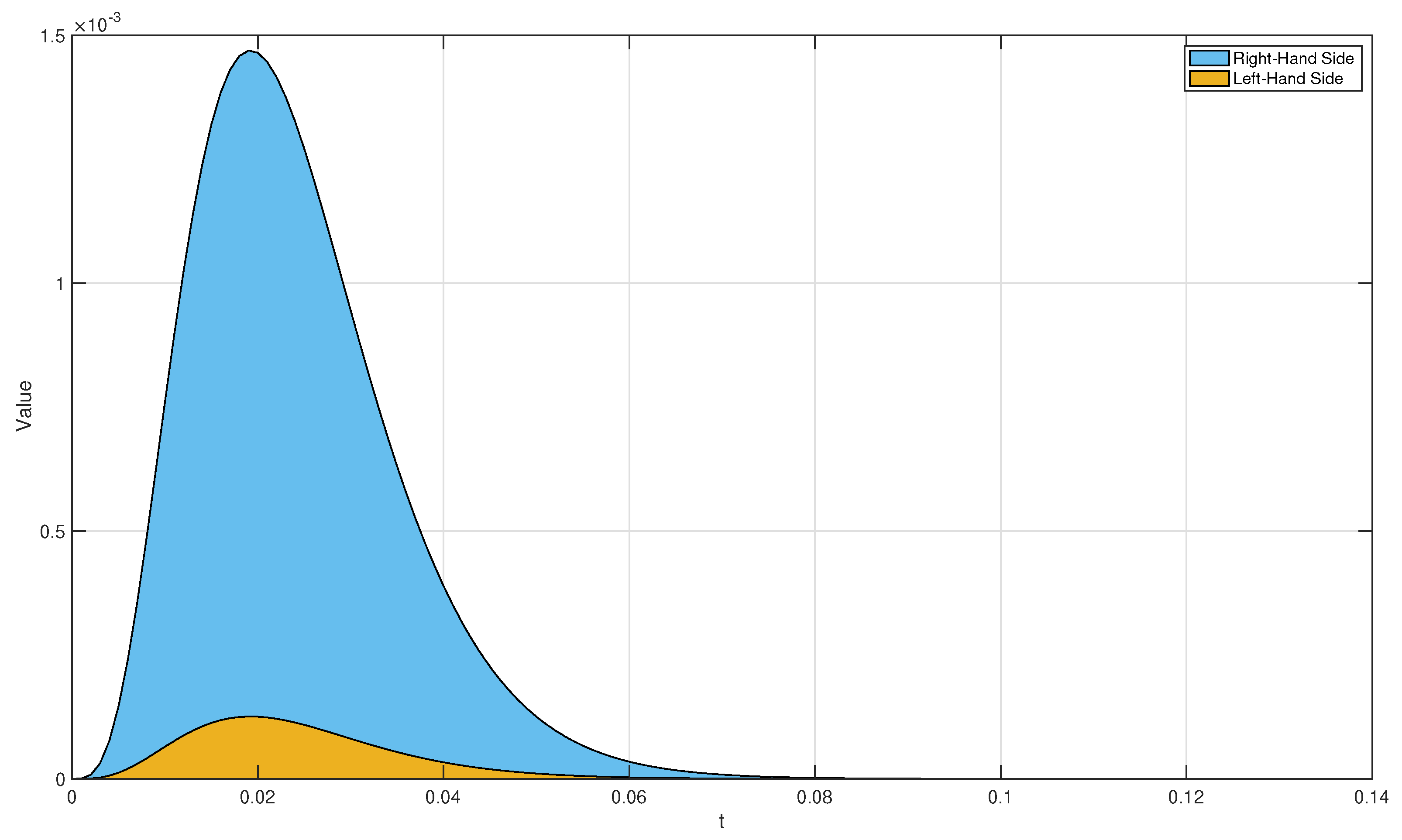
Applying Lemma 1 with ϕ ( t ) = t , α = 0.15 , ρ = 0.01 , a = 0 , and b = 0.1 , a graph representing the inequality (14) of Theorem 1 is shown in Figure 1.
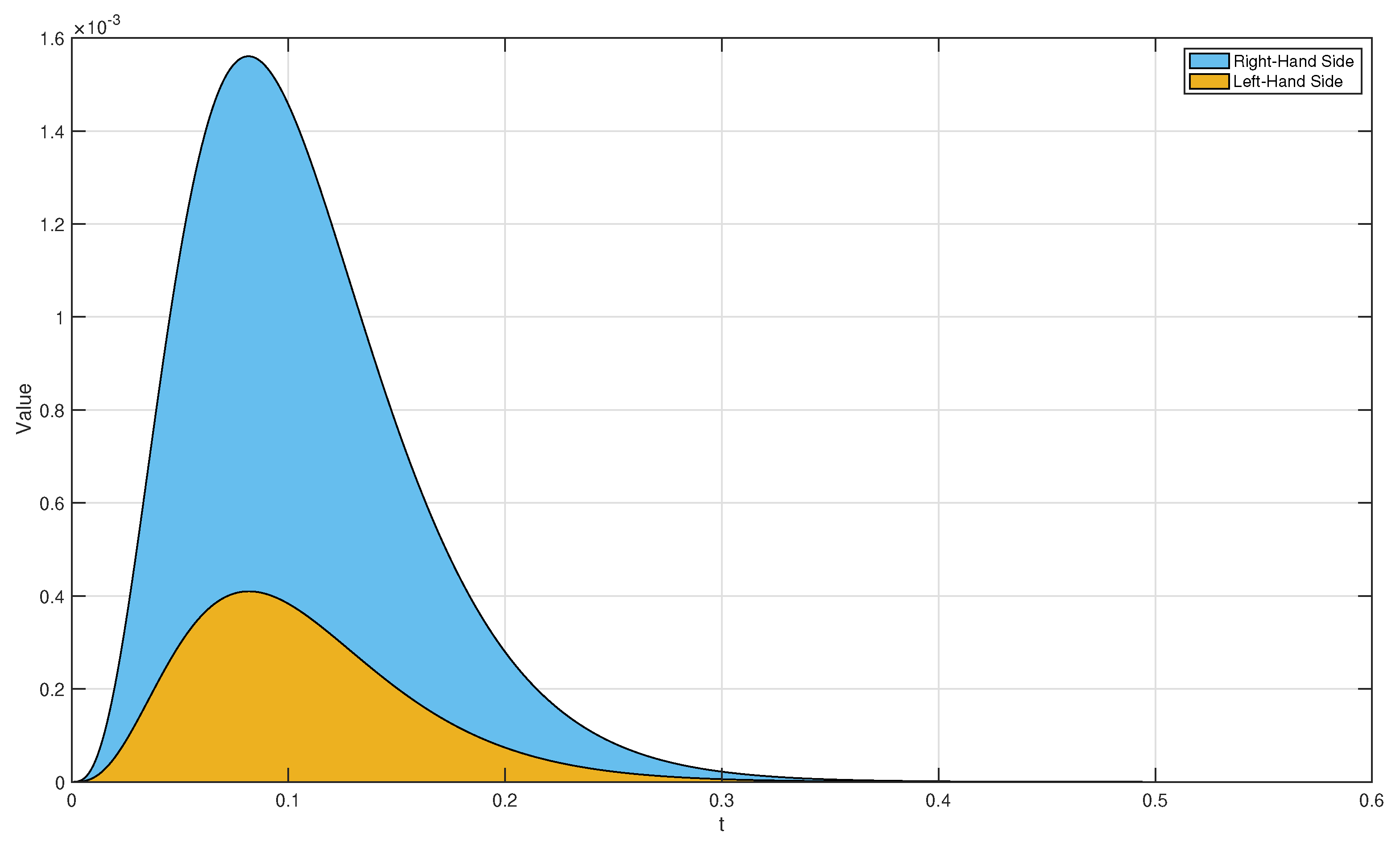
By using α = 0.9 , ρ = 0.01 , a = 0 , and b = 0.14 , a graph representing the inequality (15) of Theorem 1 is shown in Figure 2.
Remark 4.
We clearly see that if ρ = 1 and ϕ ( t ) = 1 , we have the following results:
( A 1 )
Theorem 1 ( i ) and Corollary 1 ( i ) reduce to Theorem 3.1 ( i ) and Corollary 3.4   ( i ) in [34];
( A 2 )
Corollary 1 ( i ) reduces to the first part of Theorem 1 as in [33] with α = 1 ;
( A 3 )
Corollary 1 ( i i ) reduces to the last part of Theorem 1 as in [33] with α = 1 .
( A 4 )
If we input ρ = 1 , we have Theorem 3.2 and Corollary 3.3 in [40].
Next, we are going to prove the regular form of Theorem 1 by considering two positive parameters of fractional order.
Theorem 2.
Assume that X is the C . R . V with the P . D . F   h : [ a , b ] R + . Then the following conditions hold:
( i )
For every α, β 0 and t ( a , b ] ,
ρ I a + α , ϕ [ h ( t ) ] ρ σ X , β 2 ( t ) + ρ I a + β , ϕ [ h ( t ) ] ρ σ X , α 2 ( t ) 2 ρ E X ρ E ( X ) , α ( t ) ρ E X ρ E ( X ) , β ( t ) h 2 ( ( ϕ ( t ) ϕ ( a ) ) β ρ β Γ ( β + 1 ) ρ I a + α , ϕ e ρ 1 ρ ϕ ( t ) ϕ ( t ) 2 + ( ϕ ( t ) ϕ ( a ) ) α ρ α Γ ( α + 1 ) ρ I a + β , ϕ e ρ 1 ρ ϕ ( t ) ϕ ( t ) 2 2 ρ I a + α , ϕ e ρ 1 ρ ϕ ( t ) ϕ ( t ) ρ I a + β , ϕ e ρ 1 ρ ϕ ( t ) ϕ ( t ) ) ,
where h L [ a , b ] ;
( i i )
The integral inequality
ρ I a + α , ϕ [ h ( t ) ] ρ σ X , β 2 ( t ) + ρ I a + β , ϕ [ h ( t ) ] ρ σ X , α 2 ( t ) 2 ρ E X ρ E ( X ) , α ( t ) ρ E X ρ E ( X ) , β ( t ) e ρ 1 ρ ϕ ( t ) ϕ ( t ) e ρ 1 ρ ϕ ( a ) ϕ ( a ) 2 ρ I a + α , ϕ [ h ( t ) ] ρ I a + β , ϕ [ h ( t ) ]
is also true for each α, β 0 and t ( a , b ] .
Proof. 
Inserting a function P : [ a , b ] R + , taking both sides of (17) by
1 ρ β Γ ( β ) ρ G ϕ β ( t , r ) P ( r ) ϕ ( r ) , r ( a , t ) ,
and integrating with respect to r from a to t, we obtain
1 ρ α Γ ( α ) ρ β Γ ( β ) a t a t ρ G ϕ α ( t , s ) ρ G ϕ β ( t , r ) P ( s ) P ( r ) M ( s , r ) ϕ ( s ) ϕ ( r ) d s d r = 1 ρ α Γ ( α ) a t ρ G ϕ α ( t , s ) P ( s ) g ( s ) w ( s ) ϕ ( s ) d s 1 ρ β Γ ( β ) a t ρ G ϕ β ( t , r ) P ( r ) ϕ ( r ) d r + 1 ρ α Γ ( α ) a t ρ G ϕ α ( t , s ) P ( s ) ϕ ( s ) d s 1 ρ β Γ ( β ) a t ρ G ϕ β ( t , r ) P ( r ) g ( r ) w ( r ) ϕ ( r ) d r 1 ρ α Γ ( α ) a t ρ G ϕ α ( t , s ) P ( s ) g ( s ) ϕ ( s ) d s 1 ρ α Γ ( α ) a t ρ G ϕ β ( t , r ) P ( r ) w ( r ) ϕ ( r ) d r 1 ρ α Γ ( α ) a t ρ G ϕ α ( t , s ) P ( s ) w ( s ) ϕ ( s ) d s 1 ρ β Γ ( β ) a t ρ G ϕ β ( t , r ) P ( r ) g ( r ) ϕ ( r ) d r = ρ I a + α , ϕ [ P ( t ) g ( t ) w ( t ) ] ρ I a + β , ϕ [ P ( t ) ] + ρ I a + α , ϕ [ P ( t ) ] ρ I a + β , ϕ [ P ( t ) g ( t ) w ( t ) ] ρ I a + α , ϕ [ P ( t ) g ( t ) ] ρ I a + β , ϕ [ P ( t ) w ( t ) ] ρ I a + α , ϕ [ P ( t ) w ( t ) ] ρ I a + β , ϕ [ P ( t ) g ( t ) ] .
Setting P ( s ) = h ( s ) and g ( s ) = w ( s ) = e ρ 1 ρ ϕ ( s ) ϕ ( s ) ρ E ( X ) , for t ( a , b ) , in (30), yields
1 ρ α Γ ( α ) ρ β Γ ( β ) a t a t ρ G ϕ α ( t , s ) ρ G ϕ β ( t , r ) h ( s ) h ( r ) × e ρ 1 ρ ϕ ( s ) ϕ ( s ) e ρ 1 ρ ϕ ( r ) ϕ ( r ) 2 ϕ ( s ) ϕ ( r ) d s d r = ρ I a + α , ϕ h ( t ) e ρ 1 ρ ϕ ( t ) ϕ ( t ) ρ E ( X ) 2 ρ I a + β , ϕ [ h ( t ) ] + ρ I a + α , ϕ [ h ( t ) ] ρ I a + β , ϕ h ( t ) e ρ 1 ρ ϕ ( t ) ϕ ( t ) ρ E ( X ) 2 2 ( ρ I a + α , ϕ h ( t ) e ρ 1 ρ ϕ ( t ) ϕ ( t ) ρ E ( X ) × ρ I a + β , ϕ h ( t ) e ρ 1 ρ ϕ ( t ) ϕ ( t ) ρ E ( X ) ) 2 .
Moreover, we get
1 ρ α Γ ( α ) ρ β Γ ( β ) a t a t ρ G ϕ α ( t , s ) ρ G ϕ β ( t , r ) h ( s ) h ( r ) × e ρ 1 ρ ϕ ( s ) ϕ ( s ) e ρ 1 ρ ϕ ( r ) ϕ ( r ) 2 ϕ ( s ) ϕ ( r ) d s d r h 2 ( ( ϕ ( t ) ϕ ( a ) ) β ρ β Γ ( β + 1 ) ρ I a + α , ϕ e ρ 1 ρ ϕ ( t ) ϕ ( t ) 2 + ( ϕ ( t ) ϕ ( a ) ) α ρ α Γ ( α + 1 ) ρ I a + β , ϕ e ρ 1 ρ ϕ ( t ) ϕ ( t ) 2 2 ρ I a + α , ϕ e ρ 1 ρ ϕ ( t ) ϕ ( t ) ρ I a + β , ϕ e ρ 1 ρ ϕ ( t ) ϕ ( t ) ) .
By (31) and (32), implies Theorem 2 ( i ) .
Now, we will show the Theorem 2 ( i i ) .
For s, r ( a , t ) with (30), we have
1 ρ α Γ ( α ) ρ β Γ ( β ) a t a t ρ G ϕ α ( t , s ) ρ G ϕ β ( t , r ) h ( s ) h ( r ) × e ρ 1 ρ ϕ ( s ) ϕ ( s ) e ρ 1 ρ ϕ ( r ) ϕ ( r ) 2 ϕ ( s ) ϕ ( r ) d s d r sup s , r [ a , t ] e ρ 1 ρ ϕ ( s ) ϕ ( s ) e ρ 1 ρ ϕ ( r ) ϕ ( r ) 2 × 1 ρ α Γ ( α ) a t ρ G ϕ α ( t , s ) h ( s ) ϕ ( s ) d s 1 ρ β Γ ( β ) a t ρ G ϕ β ( t , r ) h ( r ) ϕ ( r ) d r = e ρ 1 ρ ϕ ( t ) ϕ ( t ) e ρ 1 ρ ϕ ( a ) ϕ ( a ) 2 ρ I a + α , ϕ [ h ( t ) ] ρ I a + β , ϕ [ h ( t ) ] .
Hence, by (31) and (33), the inequality (29) is obtained. □
Example 2.
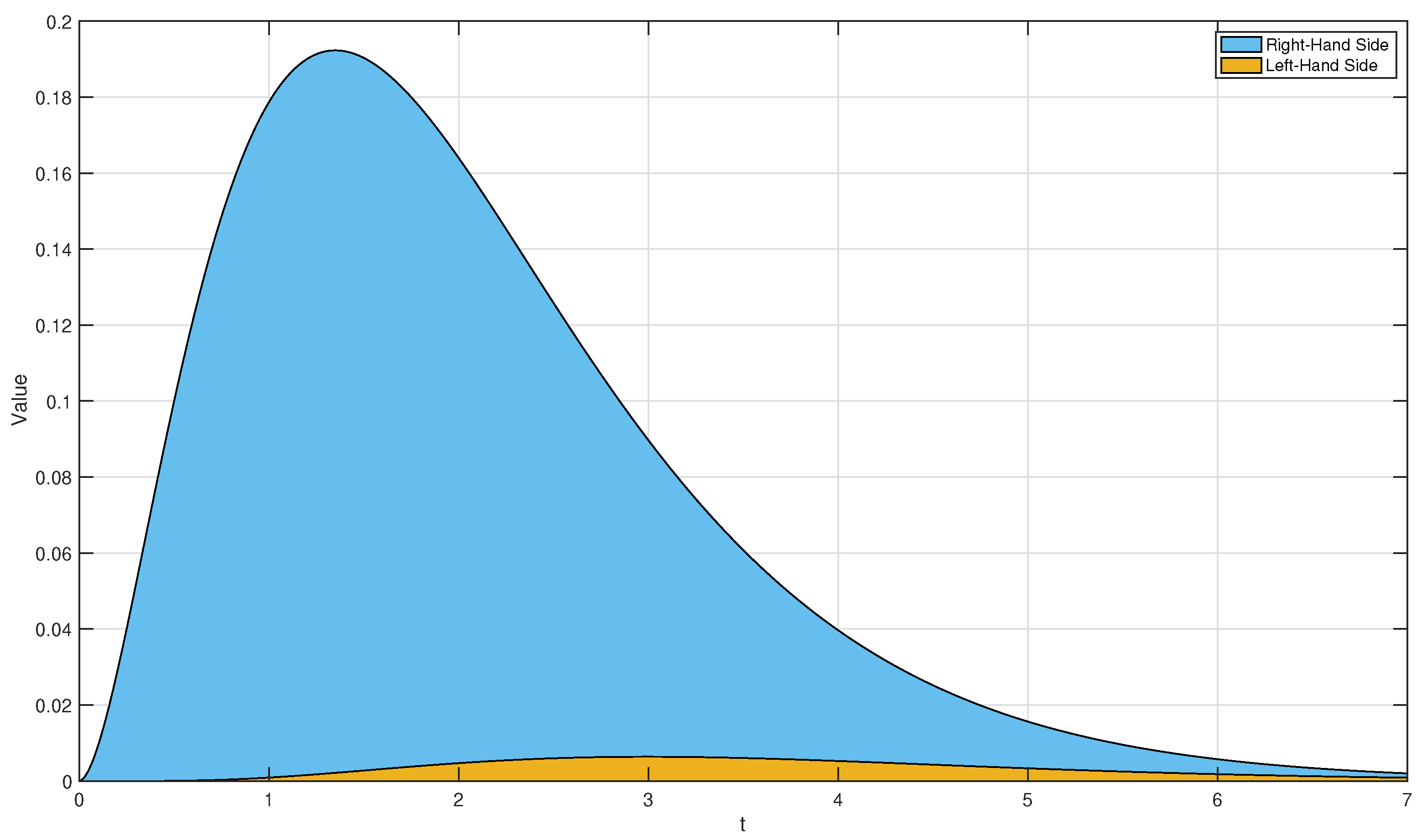
Define the P . D . F   h : [ a , b ] R + by h ( t ) = 1 / ( ϕ ( b ) ϕ ( a ) ) . Applying Lemma 1, (24,25,26,27) with ϕ ( t ) = t , α = 0.32 , β = 0.95 , ρ = 0.05 , a = 0 , and b = 0.6 , a graph representing the inequality (28) of Theorem 2 is shown in Figure 3.
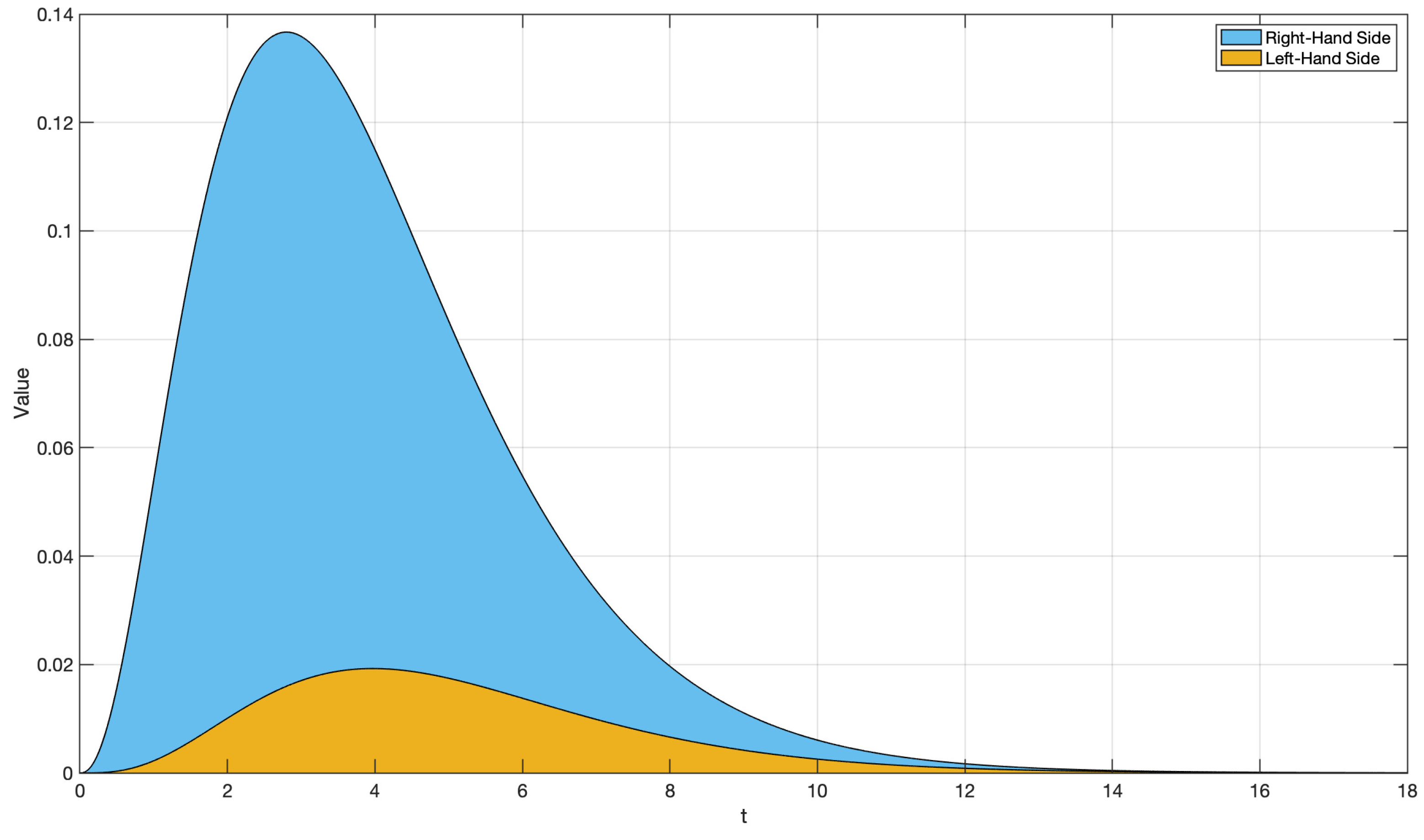
By using α = 0.9 , ρ = 0.01 , a = 0 , and b = 0.14 , a graph representing the inequality (29) of Theorem 2 is shown in Figure 4.
Remark 5.
We clearly see that:
( A 1 )
By setting α = β in Theorem 2, Theorem 2 deduces to Theorem 1;
( A 2 )
By setting ρ = 1 and ϕ ( t ) = t in Theorem 2, then Theorem 2 deduces to Theorem 3.2 in [34];
( A 3 )
By setting ρ = α = β = 1 and ϕ ( t ) = t in ( i ) of Theorem 2 then Theorem 2 deduces the first part of Theorem 1 as in [33];
( A 4 )
By setting ρ = α = β = 1 and ϕ ( t ) = t in ( i i ) of Theorem 2, then Theorem 2 deduces the last part of Theorem 1 as in [33];
( A 5 )
If we input ρ = 1 , we have Theorem 3.4 in [40].
The proportional fractional integral inequality results are shown below.
Theorem 3.
Assume that X is the C . R . V with the P . D . F   h : [ a , b ] R + . Hence
ρ I a + α , ϕ [ h ( t ) ] ρ σ X , α 2 ( t ) ρ E X ρ E ( X ) , α ( t ) 2 1 4 e ρ 1 ρ ϕ ( a ) ϕ ( b ) e ρ 1 ρ ϕ ( a ) ϕ ( a ) 2 ρ I a + α , ϕ [ h ( t ) ] 2 .
Proof. 
By applying Theorem 3.1 of [50], it follows that
ρ I a + α , ϕ [ w ( t ) ] ρ I a + α , ϕ [ w g 2 ( t ) ] ρ I a + α , ϕ [ w g ( t ) ] 2 1 4 ρ I a + α , ϕ [ w ( t ) ] 2 ( M m ) 2 .
Substituting w ( t ) = h ( t ) and g ( t ) = e ρ 1 ρ ϕ ( t ) ϕ ( t ) ϕ ( t ) ρ E ( X ) , for any t [ a , b ] , then M = e ρ 1 ρ ϕ ( b ) ϕ ( b ) ρ E ( X ) , m = e ρ 1 ρ ϕ ( a ) ϕ ( a ) ρ E ( X ) . Then (35) can be rewritten
0 ρ I a + α , ϕ [ h ( t ) ] ρ I a + α , ϕ h ( t ) e ρ 1 ρ ϕ ( t ) ϕ ( t ) ρ E ( X ) 2 ρ I a + α , ϕ h ( t ) e ρ 1 ρ ϕ ( t ) ϕ ( t ) ρ E ( X ) 2 1 4 ρ I a + α , ϕ [ h ( t ) ] 2 e ρ 1 ρ ϕ ( b ) ϕ ( b ) e ρ 1 ρ ϕ ( a ) ϕ ( a ) 2 ,
which implies that
ρ I a + α , ϕ [ h ( t ) ] ρ σ X , α 2 ( t ) ρ E X ρ E ( X ) , α ( t ) 2 1 4 e ρ 1 ρ ϕ ( b ) ϕ ( b ) e ρ 1 ρ ϕ ( a ) ϕ ( a ) 2 ρ I a + α , ϕ [ h ( t ) ] 2 .
Hence, (34) is obtained. □
If t = b , we obtain the following inequality.
Corollary 2.
Assume that X is the C . R . V with the P . D . F   h : [ a , b ] R + . Hence, for each α 0 ,
ρ G ϕ α ( b , a ) ρ α Γ ( α ) ρ σ X , α 2 ( b ) ρ E X ρ E ( X ) , α ( b ) 2 1 4 e ρ 1 ρ ϕ ( b ) ϕ ( b ) e ρ 1 ρ ϕ ( a ) ϕ ( a ) 2 ρ G ϕ α ( b , a ) ρ α Γ ( α ) 2 .
Example 3.
Define the P . D . F   h : [ a , b ] R + by h ( t ) = 1 / ( ϕ ( b ) ϕ ( a ) ) . Applying Lemma 1, (24,25,26,27) with ϕ ( t ) = t , α = 0.90 , ρ = 0.60 , a = 0 , and b = 7 , a graph representing the inequality (34) of Theorem 3 is shown in Figure 5.
Remark 6.
We clearly see that if input ρ = 1 , we have the following results:
( A 1 )
Theorem 3 and Corollary 2 deduce to Theorem 3.3 and Corollary 3.2 as in [34] with ϕ ( t ) = t ;
( A 2 )
Corollary 2 deduces to Theorem 2 as in [33] with α = 1 and ϕ ( t ) = t ;
( A 3 )
If we input ρ = 1 , we have Theorem 3.5 and Corollary 3.6 in [40].
Next, we will show the proportional F . V function with two parameters.
Theorem 4.
Assume that X is the C . R . V with the P . D . F   h : [ a , b ] R + . Hence, for each t ( a , b ] , α 0 , β 0 ,
ρ I a + α , ϕ [ h ( t ) ] ρ σ X , β ( t ) + ρ I a + β , ϕ [ h ( t ) ] ρ σ X , α ( t ) + 2 e ρ 1 ρ ϕ ( a ) ϕ ( a ) ρ E ( X ) e ρ 1 ρ ϕ ( b ) ϕ ( b ) ρ E ( X ) ρ I a + α , ϕ [ h ( t ) ] ρ I a + β , ϕ [ h ( t ) ] e ρ 1 ρ ϕ ( b ) ϕ ( b ) + e ρ 1 ρ ϕ ( a ) ϕ ( a ) 2 ρ E ( X ) × ρ I a + α , ϕ [ h ( t ) ] ρ E X ρ E ( X ) , β ( t ) + ρ I a + β , ϕ [ h ( t ) ] ρ E X ρ E ( X ) , α ( t ) .
Proof. 
By applying Theorem 3.4 of [50], we get
[ ρ I a + α , ϕ [ w ( t ) ] ρ I a + β , ϕ [ w g 2 ( t ) ] + ρ I a + β , ϕ [ w ( t ) ] ρ I a + α , ϕ [ w g 2 ( t ) ] 2 ρ I a + α , ϕ [ w ( t ) g ( t ) ] ρ I a + β , ϕ [ w g ( t ) ] ] 2 [ M ρ I a + α , ϕ [ w ( t ) ] ρ I a + α , ϕ [ w g ( t ) ] ρ I a + β , ϕ [ w g ( t ) ] m ρ I a + β , ϕ [ w ( t ) ] + ρ I a + α , ϕ [ w g ( t ) ] m ρ I a + α , ϕ [ w ( t ) ] M ρ I a + β , ϕ [ w ( t ) ] ρ I a + β , ϕ [ w g ( t ) ] ] 2 .
By substituting w ( t ) = h ( t ) , g ( t ) = e ρ 1 ρ ϕ ( t ) ϕ ( t ) ρ E ( X ) , for t [ a , b ] , then (39) can be re-written as
( ρ I a + α , ϕ [ h ( t ) ] ρ I a + β , ϕ h ( t ) e ρ 1 ρ ϕ ( t ) ϕ ( t ) ρ E ( X ) 2 + ρ I a + β , ϕ [ h ( t ) ] ρ I a + α , ϕ h ( t ) e ρ 1 ρ ϕ ( t ) ϕ ( t ) ρ E ( X ) 2 2 ρ I a + α , ϕ h ( t ) e ρ 1 ρ ϕ ( t ) ϕ ( t ) ρ E ( X ) ρ I a + β , ϕ h ( t ) e ρ 1 ρ ϕ ( t ) ϕ ( t ) ρ E ( X ) ) 2 [ M ρ I a + α , ϕ [ h ( t ) ] ρ I a + α , ϕ h ( t ) e ρ 1 ρ ϕ ( t ) ϕ ( t ) ρ E ( X ) × ρ I a + β , ϕ h ( t ) e ρ 1 ρ ϕ ( t ) ϕ ( t ) ρ E ( X ) m ρ I a + β , ϕ [ h ( t ) ] + ρ I a + α , ϕ h ( t ) e ρ 1 ρ ϕ ( t ) ϕ ( t ) ρ E ( X ) m ρ I a + α , ϕ [ h ( t ) ] × M ρ I a + β , ϕ [ h ( t ) ] ρ I a + β , ϕ h ( t ) e ρ 1 ρ ϕ ( t ) ϕ ( t ) ρ E ( X ) ] 2 .
Merging (31), (40) and using the positivity of (31) yields
ρ I a + α , ϕ [ h ( t ) ] ρ I a + β , ϕ h ( t ) e ρ 1 ρ ϕ ( t ) ϕ ( t ) ρ E ( X ) 2 + ρ I a + β , ϕ [ h ( t ) ] ρ I a + α , ϕ h ( t ) e ρ 1 ρ ϕ ( t ) ϕ ( t ) ρ E ( X ) 2 2 ρ I a + α , ϕ h ( t ) e ρ 1 ρ ϕ ( t ) ϕ ( t ) ρ E ( X ) × ρ I a + β , ϕ h ( t ) e ρ 1 ρ ϕ ( t ) ϕ ( t ) ρ E ( X ) M ρ I a + α , ϕ [ h ( t ) ] ρ I a + α , ϕ h ( t ) e ρ 1 ρ ϕ ( t ) ϕ ( t ) ρ E ( X ) × ρ I a + β , ϕ h ( t ) e ρ 1 ρ ϕ ( t ) ϕ ( t ) ρ E ( X ) m ρ I a + β , ϕ [ h ( t ) ] + ρ I a + α , ϕ h ( t ) e ρ 1 ρ ϕ ( t ) ϕ ( t ) ρ E ( X ) m ρ I a + α , ϕ [ h ( t ) ] × M ρ I a + β , ϕ [ h ( t ) ] ρ I a + β , ϕ h ( t ) e ρ 1 ρ ϕ ( t ) ϕ ( t ) ρ E ( X ) ,
which implies that
ρ I a + α , ϕ [ h ( t ) ] ρ σ X , β ( t ) + ρ I a + β , ϕ [ h ( t ) ] ρ σ X , α ( t ) + 2 m M ρ I a + α , ϕ [ h ( t ) ] ρ I a + β , ϕ [ h ( t ) ] M ρ I a + α , ϕ [ h ( t ) ] ρ E X ρ E ( X ) , β ( t ) + ρ I a + β , ϕ [ h ( t ) ] ρ E X ρ E ( X ) , α ( t ) + m ρ I a + α , ϕ [ h ( t ) ] ρ E X ρ E ( X ) , β ( t ) + ρ I a + β , ϕ [ h ( t ) ] ρ E X ρ E ( X ) , α ( t ) 2 ρ E X ρ E ( X ) , α ( t ) ρ E X ρ E ( X ) , β ( t ) .
Replacing m and M in (37) implies (38). Theorem 4 is obtained. □
Finally, if we set α = β , we have the next corollary.
Corollary 3.
Assume that X is the C . R . V with P . D . F   h : [ a , b ] R + . Hence, for each t ( a , b ] , α 0 , the inequality
ρ σ X , α ( t ) + e ρ 1 ρ ϕ ( a ) ϕ ( a ) ρ E ( X ) e ρ 1 ρ ϕ ( b ) ϕ ( b ) ρ E ( X ) ρ I a + α , ϕ [ h ( t ) ] e ρ 1 ρ ϕ ( b ) ϕ ( b ) + e ρ 1 ρ ϕ ( a ) ϕ ( a ) ρ E ( X ) ρ E X ρ E ( X ) , α ( t )
is also valid.
Example 4.
Define the P . D . F   h : [ a , b ] R + by h ( t ) = 1 / ( ϕ ( b ) ϕ ( a ) ) . Applying Lemma 1, (24,25,26,27) with ϕ ( t ) = t , α = 0.90 , β = 0.50 , ρ = 0.70 , a = 0 , and b = 18 , a graph representing the inequality (38) of Theorem 4 is shown in Figure 6.
Remark 7.
We clearly see that if we input ρ = 1 and ϕ ( t ) = t , then Theorem 4 and Corollary 3 deduce to Theorem 3.4 and Corollary 3.3 as in [34], respectively.

4. Some Examples

This section provides some proportional fractional applications for the uniform random variable X whose P . D . F   h is given for each t [ a , b ] by
h ( t ) = 1 b a .
(i)
The proportional F . E of order α : From Definition 4, we obtain that
ρ E X , α ( b ) = e ρ 1 ρ ϕ ( b ) ( ϕ ( b ) ϕ ( a ) ) α ( b a ) ρ α Γ ( α + 1 ) ϕ ( b ) α ϕ ( b ) ϕ ( a ) α + 1 .
Clearly, if α = ρ = 1 and ϕ ( t ) = t , then (43) reduces to the classical expectation of X
1 E X , 1 ( b ) = E ( X ) = a + b 2 ;
(ii)
The proportional F . M of order ( 2 , α ) : By Definition 9, one has
ρ M X 2 , α ( b ) = e ρ 1 ρ ϕ ( b ) ( ϕ ( b ) ϕ ( a ) ) α ( b a ) ρ α Γ ( α + 1 ) ( ϕ 2 ( b ) α 2 ϕ ( b ) ( ϕ ( b ) ϕ ( a ) ) α + 1 + ( ϕ ( b ) ϕ ( a ) ) 2 α + 2 ) .
Clearly, if α = ρ = 1 and ϕ ( t ) = t , then (44) reduces to the classical moment of order 2
1 M X 2 , 1 ( b ) = M 2 = a 2 + a b + b 2 3 ;
(iii)
The proportional F . V of order α : By applying Theorem 1, we obtain
ρ σ X , α 2 ( b ) = ρ M X 2 , α ( b ) 2 ρ E ( X ) ρ E X , α ( b ) + [ ρ E ( X ) ] 2 ρ I a + α , ϕ [ h ( b ) ] .
By direct computation with Definitions 3 and 4, we have
ρ I a + α , ϕ h ( b ) = 1 ρ α Γ ( α ) e ρ 1 ρ ( ϕ ( b ) ϕ ( a ) ) ( ϕ ( b ) ϕ ( a ) ) α 1
and
ρ E ( b ) = e ρ 1 ρ ϕ ( b ) ( ϕ 2 ( b ) ϕ 2 ( a ) ) 2 ( b a ) ρ .
Inserting (43), (44), (46), (47) into (45), we obtain
ρ σ X , α 2 ( b ) = e ρ 1 ρ ϕ ( b ) ( ϕ ( b ) ϕ ( a ) ) α ( b a ) ρ α Γ ( α + 1 ) { ϕ 2 ( b ) α 2 ϕ ( b ) ( ϕ ( b ) ϕ ( a ) ) α + 1 + ( ϕ ( b ) ϕ ( a ) ) 2 α + 2 e ρ 1 ρ ϕ ( b ) ( ϕ 2 ( b ) ϕ 2 ( a ) ) ( b a ) ρ [ ϕ ( b ) α ϕ ( b ) ϕ ( a ) α + 1 α e ρ 1 ρ ( ϕ ( b ) ϕ ( a ) ) ( ϕ ( b ) + ϕ ( a ) ) 4 ρ ] } .
Clearly, if α = ρ = 1 and ϕ ( t ) = t then (48) reduces to the classical varience of X
1 σ X , 1 2 ( b ) = σ 2 = ( b a ) 2 12 ;
(iv)
The proportional F . M of order ( r , α ) :
By Definition 9 and binomial expression,
( x + y ) r = k = 0 r r k x r k y k = k = 0 r r k x k y r k .
This implies that
ρ M X r , α ( b ) = k = 0 r r k Γ ( r k + 1 ) ρ α Γ ( α + r k + 1 ) e ρ 1 ρ ϕ ( a ) ϕ ( a ) k ρ G ϕ α + r k ( b , a ) .
Clearly, if α = ρ = 1 and ϕ ( t ) = t , then (49) reduces to the classical moment of order r
1 M X r , 1 ( b ) = M r = b r Γ ( r + 1 ) Γ ( r + 2 ) .

5. Conclusions

In this work, we analyzed many integral inequalities in the context of proportional RL-fractional integral operators with respect to another function under the C . R . V . The results represented extensions and enhancements of the previous results as in [33,34,36,39,40]. It is appropriate to mention that the main results can retake various previously existing operators in the special case of α = 1 . Researchers may construct a variety of variants utilizing our concepts and technique by employing the Riemann–Liouville, Hadamard, Katugampola, conformable, and proportional fractional integral operators, which result in a variety of integral inequalities for the P . D . F using various parameters and the C . R . V . In future work, it also remains to extend the results obtained to new Hilfer-type operators [51] or fractal fractional operators [52].

Author Contributions

Conceptualization, W.S., N.J., C.T. and J.K.; methodology, W.S., N.J. and J.K.; software, W.S.; validation, W.S., N.J., C.T. and J.K.; formal analysis, W.S. and N.J.; investigation, W.S., N.J., C.T. and J.K.; resources, W.S., N.J. and J.K.; data curation, W.S., N.J. and J.K.; writing—original draft preparation, W.S., N.J., C.T., J.K. and J.A.; writing—review and editing, W.S., N.J., C.T., J.K. and J.A.; visualization, W.S., N.J., C.T. and J.K.; supervision, W.S. and J.A.; project administration, W.S.; funding acquisition, N.J. All authors have read and agreed to the published version of the manuscript.

Funding

There was no external funding for this research.

Institutional Review Board Statement

Not applicable.

Informed Consent Statement

Not applicable.

Data Availability Statement

Not applicable.

Acknowledgments

W. Sudsutad was partially supported by Ramkhamhaeng University. N. Jarasthitikulchai would like to acknowledge financial support by Navamindradhiraj University through the Navamindradhiraj University Research Fund (NURF). The third and fourth authors would like to gratefully acknowledge Burapha University and the Center of Excellence in Mathematics (CEM), CHE, Sri Ayutthaya Rd., Bangkok 10400, Thailand. J. Alzabut is thankful to Prince Sultan University and OSTİM Technical University for their endless support.

Conflicts of Interest

The authors declare no conflict of interest.

Abbreviations

The following abbreviations are used in this manuscript:
FCFractional calculus
RLRiemann–Liouville
C . R . V Continuous random variable
P . D . F Probability density function
F . E Fractional expectation
F . V Fractional variance
F . M Fractional moment

References

  1. Pachpatte, B.G. Mathematical Inequalities; Elsevier: Amsterdam, The Netherlands, 2005. [Google Scholar]
  2. Cerone, P.; Dragomir, S.S. Mathematical Inequalities; CRC Press: New York, NY, USA, 2011. [Google Scholar]
  3. Guessab, A.; Schmeisser, G. Convexity results and sharp error estimates in approximate multivariate integration. Math. Comput. 2004, 73, 1365–1384. [Google Scholar] [CrossRef]
  4. Azar, S.A. Jensen’s Inequality in Finance. Int. Adv. Econ. Res. 2008, 14, 433–440. [Google Scholar] [CrossRef]
  5. Guessab, A. Direct and converse results for generalized multivariate Jensen type inequalities. J. Nonlinear Convex Anal. 2012, 13, 777–797. [Google Scholar]
  6. Sudsutad, W.; Ntouyas, S.K.; Tariboon, J. Quantum integral inequalities for convex functions. J. Math. Inequal. 2015, 9, 781–793. [Google Scholar] [CrossRef] [Green Version]
  7. Masjed-Jamei, M.; Omey, E.; Dragomir, S.S. A main class of integral inequalities with applications. Math. Model. Anal. 2016, 21, 569–584. [Google Scholar] [CrossRef]
  8. Zhao, T.H.; Wang, M.K.; Chu, Y.M. A sharp double inequality involving generalized complete elliptic integral of the first kind. AIMS Math. 2020, 5, 4512–4528. [Google Scholar] [CrossRef]
  9. Sun, M.B.; Chu, Y.M. Inequalities for the generalized weighted mean values of g-convex functions with applications. RACSAM 2020, 114, 172. [Google Scholar] [CrossRef]
  10. Khan, M.A.; Pečarić, J.; Chu, Y.M. Refinements of Jensen’s and McShane’s inequalities with applications. AIMS Math. 2020, 5, 4931–4945. [Google Scholar] [CrossRef]
  11. Sudsutad, W.; Ntouyas, S.K.; Tariboon, J. Fractional integral inequalities via Hadamard’s fractional integral. Abstr. Appl. Anal. 2014, 2014, 563096. [Google Scholar] [CrossRef]
  12. Tariboon, J.; Sudsutad, W.; Ntouyas, S.K. Some new Riemann-Liouville fractional integral inequalities. Int. J. Math. Math. Sci. 2014, 2014, 869434. [Google Scholar] [CrossRef] [Green Version]
  13. Sudsutad, W.; Ntouyas, S.K.; Tariboon, J. Integral inequalities via fractional quantum calculus. J. Inequal. Appl. 2016, 2016, 81. [Google Scholar] [CrossRef] [Green Version]
  14. Kacar, E.; Kacar, Z.; Yildirim, H. Integral inequalities for Riemann-Liouville fractional integrals of a function with respect to another function. Iran. J. Math. Sci. Inform. 2018, 13, 1–13. [Google Scholar]
  15. Alzabut, J.; Abdeljawad, T.; Jarad, F.; Sudsutad, W. A Gronwall inequality via the generalized proportional fractional derivative with applications. J. Inequal. Appl. 2019, 2019, 101. [Google Scholar] [CrossRef] [Green Version]
  16. Abdeljawad, T.; Jarad, F.; Mallak, S.; Alzabut, J. Lyapunov type inequalities via fractional proportional derivatives and application on the free zero disc of Kilbas-Saigo generalized Mittag-Leffler functions. Eur. Phys. J. Plus 2019, 134, 247. [Google Scholar] [CrossRef]
  17. Alzabut, J.; Sudsutad, W.; Kayar, Z.; Baghani, H. A new Gronwall-Bellman inequality in frame of generalized proportional fractional derivative. Mathematics 2019, 7, 747. [Google Scholar] [CrossRef] [Green Version]
  18. Xu, L.; Chu, Y.M.; Rashid, S.; El-Deeb, A.A.; Nisar, K.S. On new unified bounds for a family of functions with fractional q-calculus theory. J. Funct. Spaces 2020, 2020, 4984612. [Google Scholar]
  19. Abdeljawad, T.; Rashid, S.; Hammouch, Z.; Chu, Y.M. Some new local fractional inequalities associated with generalized (s, m)-convex functions and applications. Adv. Differ. Equ. 2020, 2020, 406. [Google Scholar] [CrossRef]
  20. Guo, S.Y.; Chu, Y.M.; Farid, G.; Mehmood, S.; Nazeer, W. Fractional Hadamard and Fejér-Hadamard inequaities associated with exponentially (s, m)-convex functions. J. Funct. Spaces 2020, 2020, 2410385. [Google Scholar]
  21. Rashid, S.; Noor, M.A.; Noor, K.I.; Chu, Y.M. Ostrowski type inequalities in the sense of generalized K-fractional integral operator for exponentially convex functions. AIMS Math. 2020, 5, 2629–2645. [Google Scholar] [CrossRef]
  22. Khurshid, Y.; Khan, M.A.; Chu, Y.M. Conformable integral version of Hermite-Hadamard-Fejér inequalities via η-convex functions. AIMS Math. 2020, 5, 5106–5120. [Google Scholar] [CrossRef]
  23. Rashid, S.; Khalid, A.; Rahman, G.; Nisar, K.S.; Chu, Y.M. On new modifications governed by quantum Hahn’s integral operator pertaining to fractional calculus. J. Funct. Spaces 2020, 2020, 8262860. [Google Scholar] [CrossRef]
  24. Rashid, S.; Jarad, F.; Chu, Y.M. A note on reverse Minkowski inequality via generalized proportional fractional integral operator with respect to another function. Math. Probl. Eng. 2020, 2020, 7630260. [Google Scholar] [CrossRef]
  25. Kilbas, A.A.; Srivastava, H.M.; Trujillo, J.J. Theory and Applications of Fractional Differential Equations; Elsevier: Amsterdam, The Netherlands, 2006. [Google Scholar]
  26. Katugampola, U.N. New approach to generalized fractional integral. Appl. Math. Comput. 2011, 218, 860–865. [Google Scholar] [CrossRef] [Green Version]
  27. Abdeljawad, T. On conformable fractional calculus. J. Comput. Appl. Math. 2015, 279, 57–66. [Google Scholar] [CrossRef]
  28. Jarad, F.; Uǧurlu, E.; Abdeljawad, T.; Baleanu, D. On a new class of fractional operators. Adv. Differ. Equ. 2017, 2017, 247. [Google Scholar] [CrossRef]
  29. Khan, T.U.; Khan, M.A. Generalized conformable fractional operators. J. Comput. Appl. Math. 2019, 346, 378–389. [Google Scholar] [CrossRef]
  30. Jarad, F.; Alqudah, M.A.; Abdeljawad, T. On more generalized form of proportional fractional operators. Open Math. 2020, 18, 167–176. [Google Scholar] [CrossRef] [Green Version]
  31. Jarad, F.; Abdeljawad, T.; Rashid, S.; Hammouch, Z. More properties of the proportional fractional integrals and derivatives of a function with respect to another function. Adv. Differ. Equ. 2020, 2020, 303. [Google Scholar] [CrossRef]
  32. Barnett, N.S.; Dragomir, S.S. Some inequalities for random variables whose probability density functions are bounded using a pre-Grüss inequality. Kyungpook Math. J. 2020, 40, 299–311. [Google Scholar]
  33. Barnett, N.S.; Cerone, P.; Dargomir, S.S.; Roumeliotis, J. Some inequalities for the expectation and variance of a random variable whose PDF is n-time differentiable. J. Inequal. Pure Appl. Math. 2000, 2, 1–18. [Google Scholar]
  34. Dahmani, Z. Fractional integral inequalities for continous random variables. Malaya J. Mat. 2014, 2, 172–179. [Google Scholar]
  35. Akkurt, A.; Kaçar, Z.; Yildirim, H. Generalized fractional integral inequalities for continuous random variables. J. Prob. Stat. 2015, 2015, 958980. [Google Scholar] [CrossRef] [Green Version]
  36. Dahmani, Z. New applications of fractional calculus on probabilistic random variables. Acta Math. Univ. Comen. 2017, LXXXVI, 299–307. [Google Scholar]
  37. Dahmani, Z.; Khameli, A.; Bezziou, M.; Sarikaya, M.Z. Some estimations on continuous random variables involving fractional calculus. Int. J. Anal. Appl. 2017, 15, 8–17. [Google Scholar]
  38. Dahmani, Z.; Bouziane, A.E.; Houas, M.; Sarikaya, M.Z. New w-weighted concepts for continuous random variables with applications. Note di Mat. 2017, 37, 23–40. [Google Scholar]
  39. Khellaf, O.M.; Chinchane, V.L. Continuous random variables with Hadamard fractional integral. Tamkang J. Math. 2019, 50, 103–109. [Google Scholar]
  40. Chen, S.B.; Rashid, S.; Noor, M.A.; Ashraf, R.; Chu, Y.M. A new approach on fractional calculus and probability density function. AIMS Math. 2020, 5, 7041–7054. [Google Scholar] [CrossRef]
  41. Houas, M. Some estimations on continuous random variables for (k, s)-fractional integral operators. Moroc. J. Pure Appl. Anal. 2020, 6, 143–154. [Google Scholar] [CrossRef]
  42. Houas, M. Some inequalities for k-fractional continuous random variables. J. Adv. Res. Dyn. Control Syst. 2015, 7, 43–50. [Google Scholar]
  43. Tomar, M.; Maden, S.; Set, E. (k, s)-Riemann-Liouville fractional integral inequalities for continuous random variables. Arab. J. Math. 2017, 6, 55–63. [Google Scholar] [CrossRef] [Green Version]
  44. Houas, M.; Dahmani, Z.; Sarikaya, M.Z. New integral inequalities for (r, α)-fractional moments of continuous random variables. Mathematica 2018, 60, 166–176. [Google Scholar] [CrossRef]
  45. Sarikaya, M.Z.; Dahmani, Z.; Kiris, M.E.; Ahmad, F. (k, s)-Riemann-Liouville fractional integral and applications. Hacet. J. Math. Stat. 2016, 45, 77–89. [Google Scholar] [CrossRef]
  46. Bounoua, M.D.; Dahmani, Z.; Bekkouche, Z. Further results and applications on continuous random variables. Malaya J. Mat. 2019, 7, 429–435. [Google Scholar] [CrossRef] [Green Version]
  47. Abdelnebi, A.; Dahmani, Z.; Sarikaya, M.Z. New classes of fractional integral inequalities and some recent results on random variables. Malaya J. Mat. 2020, 8, 738–743. [Google Scholar] [CrossRef]
  48. Cerone, P.; Dargomir, S.S. On some inequalities for the expectation and variance. Korean J. Comput. Appl. Math. 2001, 8, 357–380. [Google Scholar] [CrossRef] [Green Version]
  49. Kumar, P. Inequalities involving moments of a continuous random variable defined over a finite interval. Comput. Math. Appl. 2004, 48, 257–273. [Google Scholar] [CrossRef]
  50. Dahmani, Z.; Tabharit, L. On weighted Gruss type inequalities via fractional integrals. J. Adv. Res. Pure Math. 2010, 2, 31–38. [Google Scholar] [CrossRef]
  51. Nápoles, V.J.E. Generalized fractional Hilfer integral and derivative. Contrib. Math. 2020, 2, 55–60. [Google Scholar]
  52. Atangana, A. Fractal-fractional differentiation and integration: Connecting fractal calculus and fractional calculus to predict complex system. Chaos Solitons Fractals 2017, 102, 396–406. [Google Scholar] [CrossRef]
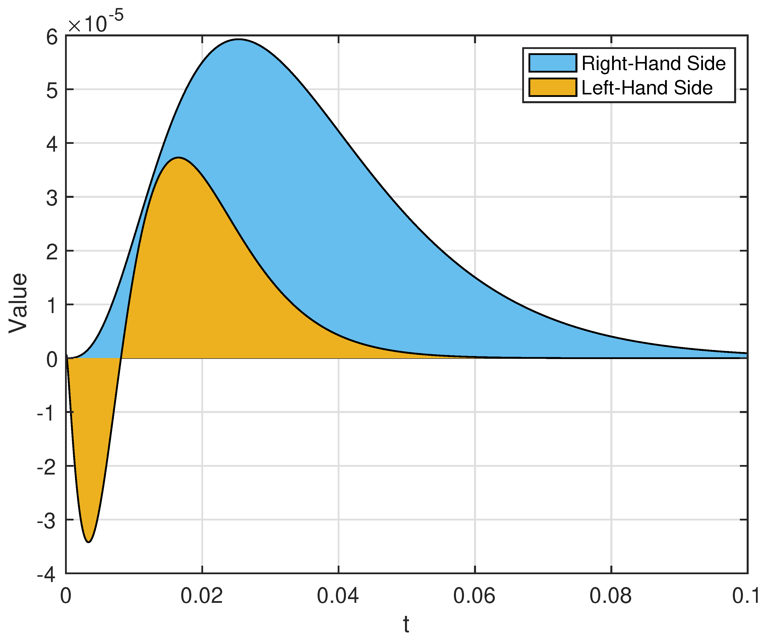
Figure 1. The graph of the inequality (14).
Mathematics 10 00573 g001
Figure 2. The graph of the inequality (15).
Mathematics 10 00573 g002
Figure 3. The graph of the inequality (28).
Mathematics 10 00573 g003
Figure 4. The graph of the inequality (29).
Mathematics 10 00573 g004
Figure 5. The graph of the inequality (34).
Mathematics 10 00573 g005
Figure 6. The graph of the inequality (38).
Mathematics 10 00573 g006
Publisher’s Note: MDPI stays neutral with regard to jurisdictional claims in published maps and institutional affiliations.