Author Contributions
Conceptualisation, A.J., C.M.A., G.P.; methodology, A.J.; software, A.J., M.A.F.G., C.M.A.; validation, A.J.; formal analysis, A.J.; investigation, A.J.; data curation, A.J., M.A.F.G.; writing—original draft preparation, A.J.; writing—review and editing, A.J., M.A.F.G., C.M.A., G.P.; visualisation, A.J., M.A.F.G.; funding acquisition, A.J., C.M.A. All authors have read and agreed to the published version of the manuscript.
Figure 1.
(
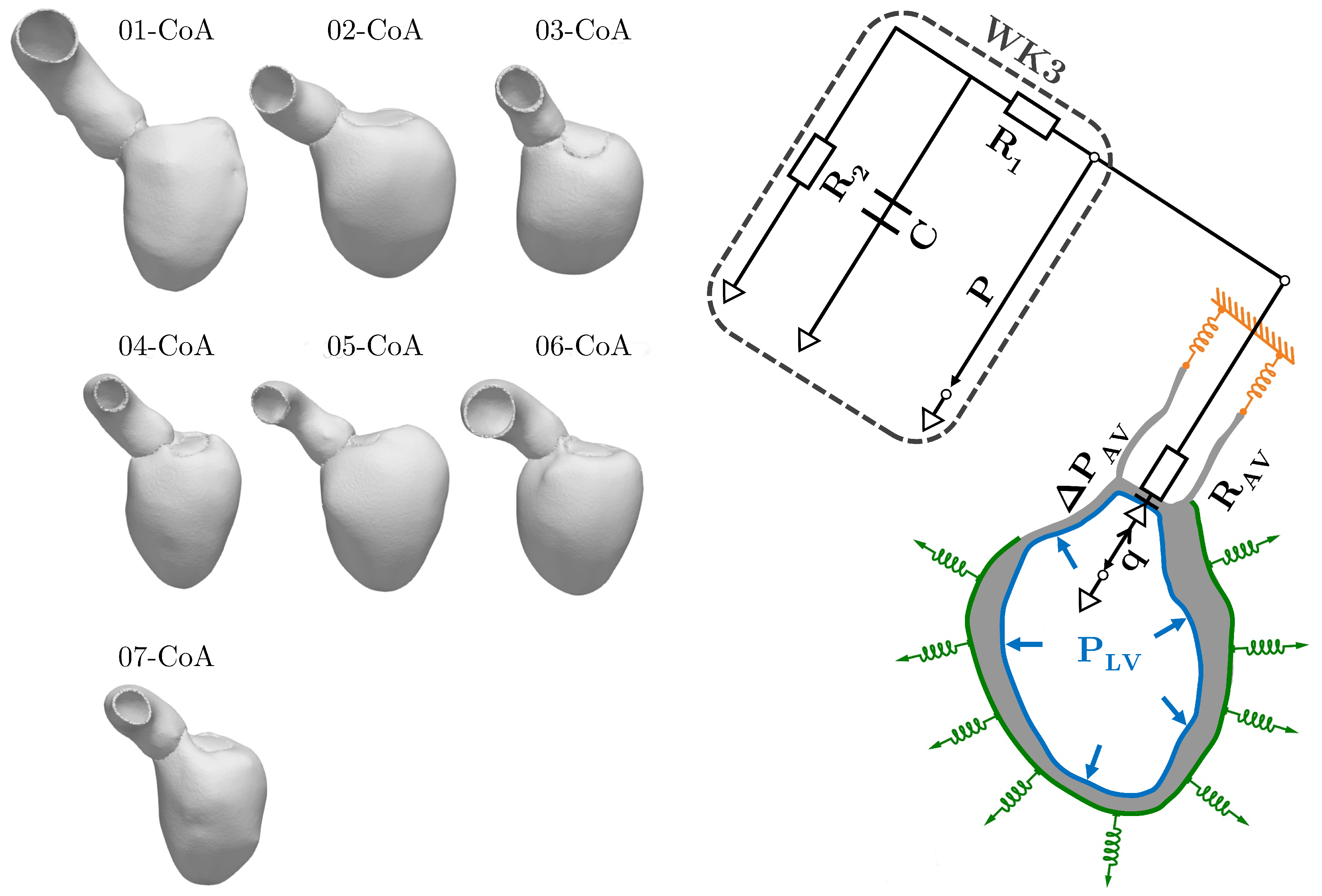
Left), seven patient-specific anatomical models of the left ventricle (LV) and the aortic root from patients treated for aortic coarctation (CoA); (
right), mechanical and afterload boundary conditions where Neumann-type pressure boundary conditions are illustrated in blue and Robin-type boundary conditions are illustrated in green (uni-directional springs that mimic the effect of the pericardium) and yellow (omni-directional springs). The mechanical model is coupled to a 0D three-element Windkessel model (WK3) that accounts for afterload conditions. Here,
,
are the characteristic and peripheral resistances, respectively, and
C is the arterial compliance. Pressure is denoted by
P and the relationship between pressure and flow
across the aortic valve (AV) is represented by a 0D diode model, where
is the respective resistance. The diode model of the flow across the mitral valve and the uni-directional springs that are applied to the septum are not shown. See [
18] for more details.
Figure 1.
(
Left), seven patient-specific anatomical models of the left ventricle (LV) and the aortic root from patients treated for aortic coarctation (CoA); (
right), mechanical and afterload boundary conditions where Neumann-type pressure boundary conditions are illustrated in blue and Robin-type boundary conditions are illustrated in green (uni-directional springs that mimic the effect of the pericardium) and yellow (omni-directional springs). The mechanical model is coupled to a 0D three-element Windkessel model (WK3) that accounts for afterload conditions. Here,
,
are the characteristic and peripheral resistances, respectively, and
C is the arterial compliance. Pressure is denoted by
P and the relationship between pressure and flow
across the aortic valve (AV) is represented by a 0D diode model, where
is the respective resistance. The diode model of the flow across the mitral valve and the uni-directional springs that are applied to the septum are not shown. See [
18] for more details.
![Mathematics 10 00823 g001]()
Figure 2.
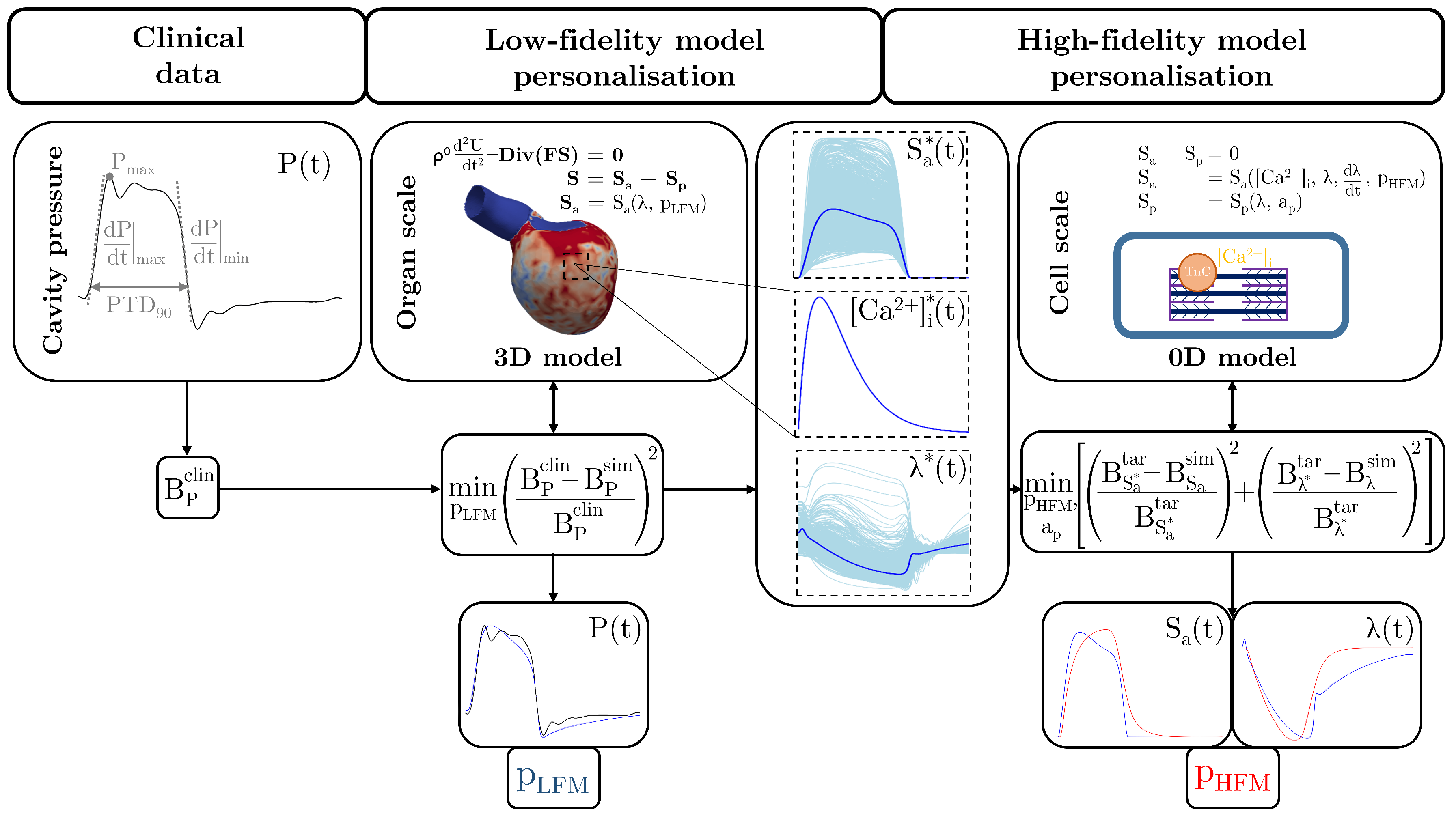
Conceptual illustration of the two-step multi-fidelity approach for personalising biophysically detailed active mechanics models. In the first step, the active mechanical behaviour in the given 3D EM model is described by a low-fidelity model (LFM). This is personalised at the organ scale by minimising the difference between simulated (sim) and clinical (clin) pressure biomarker values (
) that are obtained from an available clinical cavity pressure trace. Median traces of nodal cellular active stress (
), intracellular calcium concentration (
), and fibre stretch (
) are then obtained from the simulation that was produced by the personalised 3D EM models. These are utilised to personalise the high-fidelity model (HFM) at the cell scale in the second step. To this end, the HFM model is integrated in an 0D EM model that simulates the stretch of the cardiomyocyte during the cardiac cycle based on the equilibrium of active and passive stress. The median trace of nodal
is used as input but
can also be generated from a coupled model of
evolution that is integrated in the chosen cellular EP model. Personalisation is done by minimising the difference between simulated (sim) and target (tar) biomarker values that are obtained from the median traces of nodal cellular active stress (
) and fibre stretch (
). The parameters of the LFM and the HFM are denoted by
and
, respectively. Please note that the fibre stretch in the relaxed state is 1 per definition (
Section 2.3.1 and
Appendix A.3).
Figure 2.
Conceptual illustration of the two-step multi-fidelity approach for personalising biophysically detailed active mechanics models. In the first step, the active mechanical behaviour in the given 3D EM model is described by a low-fidelity model (LFM). This is personalised at the organ scale by minimising the difference between simulated (sim) and clinical (clin) pressure biomarker values (
) that are obtained from an available clinical cavity pressure trace. Median traces of nodal cellular active stress (
), intracellular calcium concentration (
), and fibre stretch (
) are then obtained from the simulation that was produced by the personalised 3D EM models. These are utilised to personalise the high-fidelity model (HFM) at the cell scale in the second step. To this end, the HFM model is integrated in an 0D EM model that simulates the stretch of the cardiomyocyte during the cardiac cycle based on the equilibrium of active and passive stress. The median trace of nodal
is used as input but
can also be generated from a coupled model of
evolution that is integrated in the chosen cellular EP model. Personalisation is done by minimising the difference between simulated (sim) and target (tar) biomarker values that are obtained from the median traces of nodal cellular active stress (
) and fibre stretch (
). The parameters of the LFM and the HFM are denoted by
and
, respectively. Please note that the fibre stretch in the relaxed state is 1 per definition (
Section 2.3.1 and
Appendix A.3).
![Mathematics 10 00823 g002]()
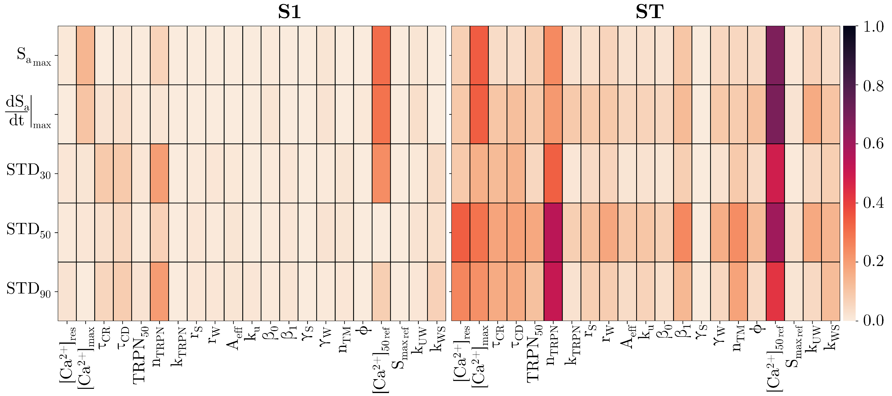
Figure 3.
Global sensitivity of active stress biomarkers to parameters of the Land and the Rice model in the 0D EM model. The Sobol global sensitivity analysis was performed and first-order () and total-order sensitivity indices () are shown.
Figure 3.
Global sensitivity of active stress biomarkers to parameters of the Land and the Rice model in the 0D EM model. The Sobol global sensitivity analysis was performed and first-order () and total-order sensitivity indices () are shown.
Figure 4.
Comparison of simulated and clinical left ventricular pressure and volume after personalisation. The blue/red lines represent the simulation data Sim1/Sim2 that were produced by the 3D model of human left ventricular EM in the first/second step of the active mechanics personalisation approach. The black dots represent clinical data (Clin). (a) Pressure–volume loops, (b) pressure traces, and (c) volume traces are shown.
Figure 5.
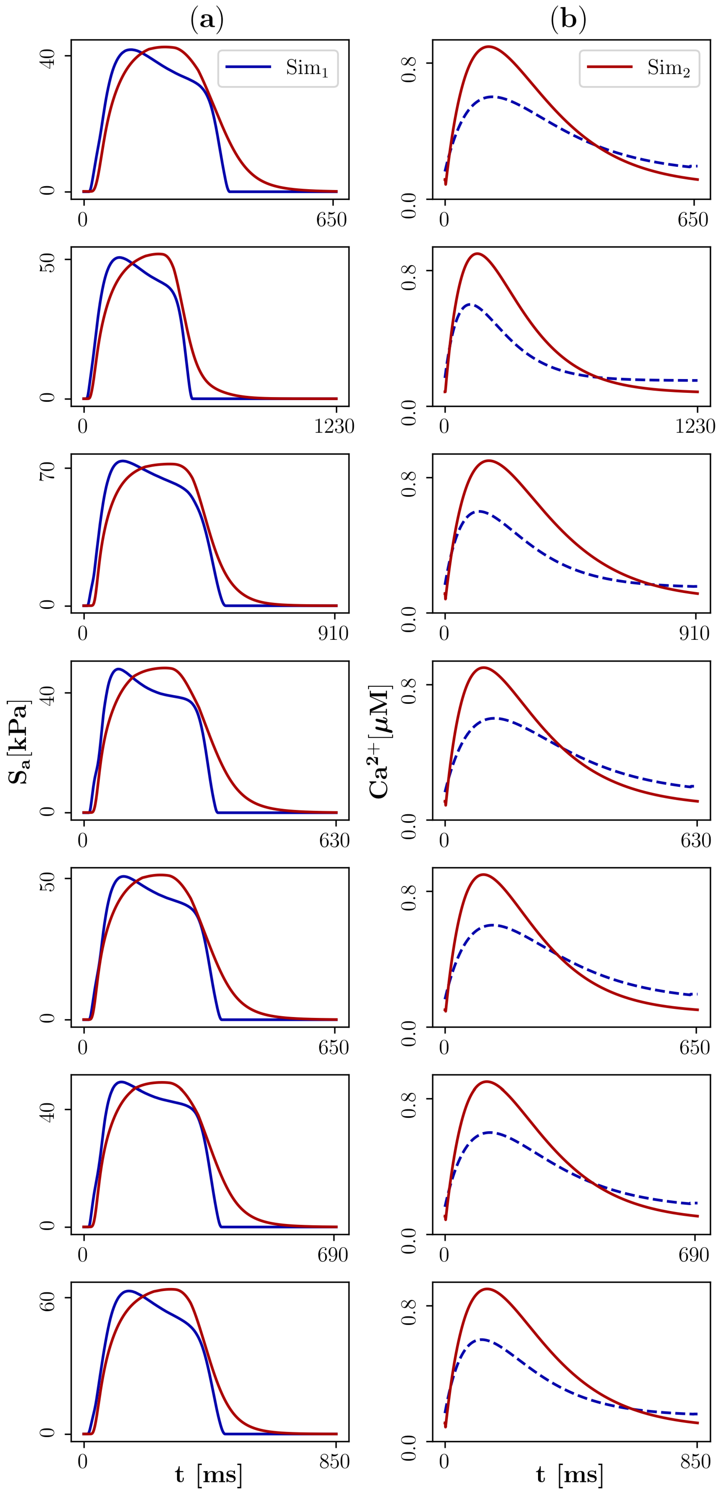
Comparison of simulated cellular active stress and intracellular calcium concentration. The blue lines represent the median nodal traces obtained from the simulations that were produced by the 3D model of human left ventricular EM in the first step (Sim1). The red lines represent the traces that were produced by the 0D model of cellular EM in the second step of the active mechanics personalisation approach (Sim2). (a) Cellular active stress traces (solid line represents a target for the personalisation), (b) intracellular calcium concentration traces (dashed line does not represent a target for the personalisation).
Figure 5.
Comparison of simulated cellular active stress and intracellular calcium concentration. The blue lines represent the median nodal traces obtained from the simulations that were produced by the 3D model of human left ventricular EM in the first step (Sim1). The red lines represent the traces that were produced by the 0D model of cellular EM in the second step of the active mechanics personalisation approach (Sim2). (a) Cellular active stress traces (solid line represents a target for the personalisation), (b) intracellular calcium concentration traces (dashed line does not represent a target for the personalisation).
Figure 6.
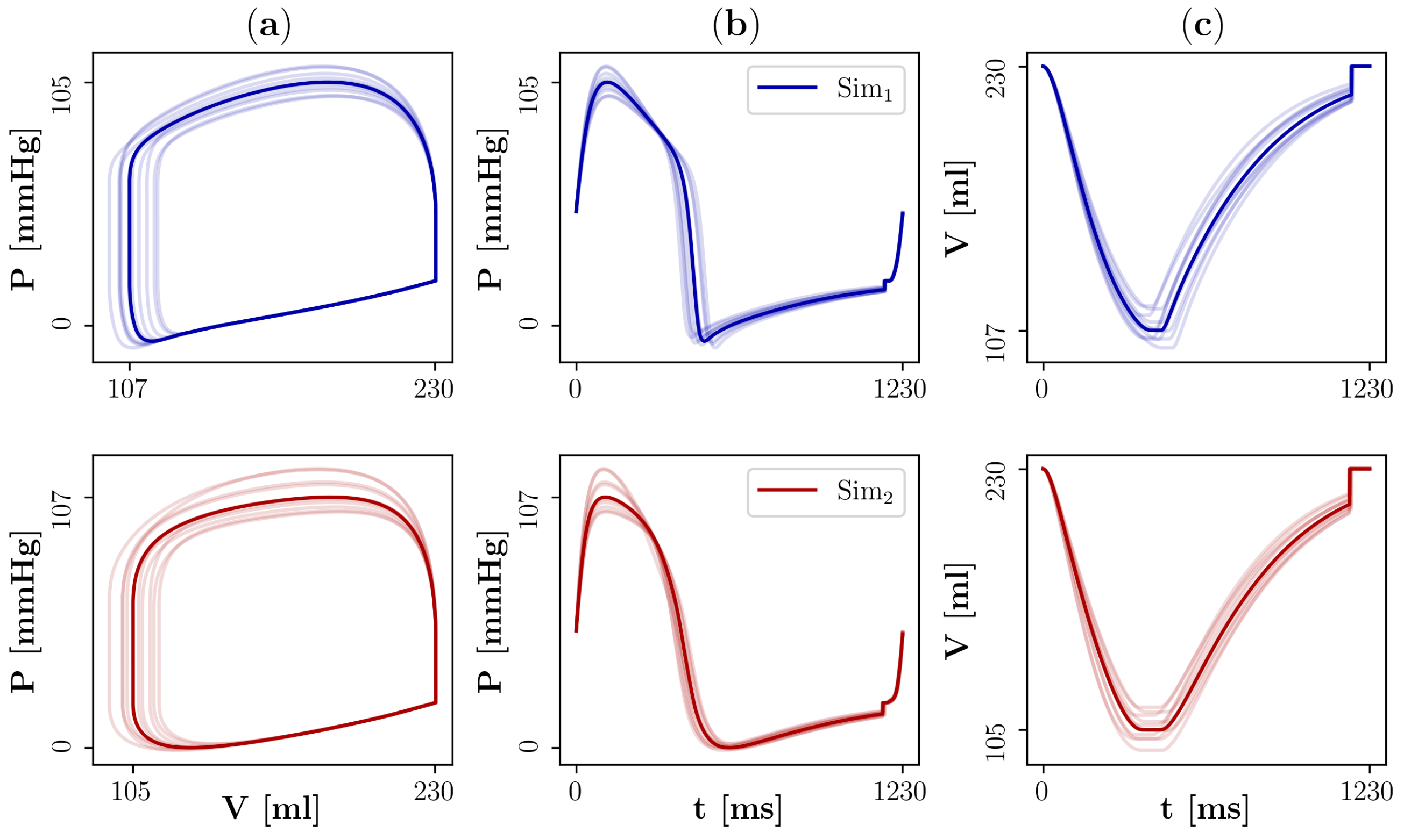
Effect of clinical data uncertainty on simulated left ventricular pressure and volume in the two steps of the active mechanics personalisation approach. The blue/red lines represent the simulation data (Sim1, Sim2) that were produced by the 3D model of human left ventricular EM in the first/second step of the active mechanics personalisation approach. The active mechanics personalisation was performed based on ten samples of clinical biomarkers (±10% around the measured value) and the resulting pressures and volumes (light colours) are compared to those that resulted from the personalisation based on the measured values (bold colours). (a) Pressure–volume loops, (b) pressure traces, (c) volume traces.
Figure 6.
Effect of clinical data uncertainty on simulated left ventricular pressure and volume in the two steps of the active mechanics personalisation approach. The blue/red lines represent the simulation data (Sim1, Sim2) that were produced by the 3D model of human left ventricular EM in the first/second step of the active mechanics personalisation approach. The active mechanics personalisation was performed based on ten samples of clinical biomarkers (±10% around the measured value) and the resulting pressures and volumes (light colours) are compared to those that resulted from the personalisation based on the measured values (bold colours). (a) Pressure–volume loops, (b) pressure traces, (c) volume traces.
Table 1.
Mesh information, CPU times, and iteration numbers for each patient case. Given is the number of nodes and elements of the patient-specific FE mesh, the cardiac cycle length, and the times per iteration and number of iterations for personalising the low-fidelity model (LFM) in the first step (3D EM model) and the high fidelity model (HFM) in the second step (0D EM model). 3D simulations in the first step were run on ARCHER2 using 128 cores and 0D simulations in the second step were run on a desktop computer using 1 core.
| Patient Case | # Nodes | # Elements | Cycle Length | Time/It LFM | Time/It HFM | # It LFM | # It HFM |
|---|
| (-) | (-) | (ms) | (s) | (s) | (-) | (-) |
|---|
| 01-CoA | 159,948 | 806,430 | 659 | 4834.7 | 0.033 | 2 | 13,211 |
| 02-CoA | 162,188 | 835,516 | 1231 | 7945.4 | 0.061 | 3 | 16,061 |
| 03-CoA | 63,804 | 301,146 | 917 | 2389.4 | 0.045 | 4 | 17,261 |
| 04-CoA | 96,176 | 487,132 | 631 | 2249.1 | 0.031 | 9 | 8561 |
| 05-CoA | 126,981 | 652,012 | 654 | 3434.8 | 0.032 | 3 | 16,211 |
| 06-CoA | 165,508 | 853,717 | 697 | 5407.9 | 0.036 | 4 | 14,111 |
| 07-CoA | 82,212 | 394,690 | 852 | 2591.8 | 0.042 | 3 | 20,766 |
Table 2.
Simulated and clinical LV pressure and volume biomarker values for each patient case. Clinical data are given in the first panel and results of the first and the second step of the active mechanics personalisation approach are given in the second and third panel. The goodness of fit is measured as relative difference between simulated and clinical value and given in brackets.
| Patient Case | Pmax | | | PTD90 | SV |
|---|
| (mmHg) | (mmHg ms) | (mmHg ms) | (ms) | (mL) |
|---|
| | 119 | 2.7 | −2.9 | 309 | 100 |
| 01-CoA | 115 (3.0%) | 1.9 (30.9%) | −2.2 (26.7%) | 330 (6.7%) | 90 (10.4%) |
| | 125 (5.1%) | 2.8 (3.7%) | −1.2 (59.4%) | 316 (2.1%) | 92.6 (7.4%) |
| | 105 | 1.3 | −1.5 | 452 | 115 |
| 02-CoA | 105 (<0.1%) | 1.2 (5.3%) | −1.5 (2.5%) | 460 (1.9%) | 123 (6.8%) |
| | 107 (1.5%) | 1.5 (18.5%) | −0.9 (39.8%) | 446 (1.2%) | 126 (8.6%) |
| | 121 | 1.9 | −1.2 | 450 | 46 |
| 03-CoA | 114 (5.7%) | 1.7 (12.7%) | −1.3 (5.4%) | 448 (0.3%) | 46 (0.1%) |
| | 112 (7.8%) | 2.5 (28.7%) | −1.2 (1.2%) | 431 (4.1%) | 44 (4.0%) |
| | 129 | 3.6 | −3.1 | 290 | 68 |
| 04-CoA | 126 (2.7%) | 3.2 (12.0%) | −3.1 (0.9%) | 290 (<0.1%) | 53 (20.9%) |
| | 126 (2.6%) | 3.8 (5.7%) | −1.3 (55.8%) | 302 (4.1%) | 52 (23.6%) |
| 133 | 2.7 | −2.3 | 309 | 92 |
| 05-CoA | 120 (10.1%) | 2.4 (13.8%) | −2.5 (5.7%) | 309 (0.2%) | 81 (11.5%) |
| | 123 (7.4%) | 3.4 (22.9%) | −1.1 (54.1%) | 310 (0.5%) | 83 (10.1%) |
| | 152 | 3.2 | −2.7 | 332 | 100 |
| 06-CoA | 139 (8.7%) | 2.7 (15.2%) | −2.8 (6.3%) | 332 (0.1%) | 87 (12.5%) |
| | 142 (6.4%) | 3.4 (6.8%) | −1.2 (54.4%) | 345 (4.1%) | 83 (16.5%) |
| | 110 | 1.2 | −1.2 | 412 | 55 |
| 07-CoA | 101 (7.7%) | 1.3 (5.2%) | −1.2 (6.3%) | 409 (0.6%) | 60 (7.6%) |
| | 101 (7.5%) | 2.1 (71.2%) | −1.0 (14.7%) | 394 (4.3%) | 59 (7.5%) |
Table 3.
Results of the clinical data uncertainty robustness analysis for the patient case 02-CoA. Estimated model parameter values of the first step of the active mechanics personalisation approach are given. The original values are listed in the first row and means (M), standard deviations (SD), minima (Min), and maxima (Max) of ten samples are listed in the subsequent rows. Means, standard deviations, minima, and maxima of the relative differences are given in brackets below.
| | Smaxref | | | TCR | RAVf | RMVf |
|---|
| | (kPa) | (ms) | (ms) | (ms) | (mmHg mL s) | (mmHg mL s) |
|---|
| Original | 103.2 | 30.1 | 48.8 | 529.3 | 0.0125 | 0.0794 |
| Mean | 103.4 | 30.7 | 48.3 | 524.9 | 0.0112 | 0.0795 |
| (7.8%) | (8.0%) | (4.6%) | (5.0%) | (10.8%) | (5.0%) |
| SD | 9.4 | 2.6 | 2.7 | 30.3 | 0.0015 | 0.0048 |
| (4.8%) | (3.2%) | (3.2%) | (2.9%) | (8.1%) | (3.3%) |
| Min | 88.9 | 26.5 | 43.7 | 478.9 | 0.0090 | 0.0728 |
| (0.9%) | (2.8%) | (0.1%) | (0.4%) | (0.4%) | (<0.1%) |
| Max | 118.8 | 33.6 | 51.9 | 572.2 | 0.0138 | 0.0878 |
| (15.1%) | (13.9%) | (10.4%) | (9.5%) | (23.0%) | (10.6%) |
Table 4.
Results of the clinical data uncertainty robustness analysis for the patient case 02-CoA. LV pressure and volume biomarker values of the first step of the active mechanics personalisation approach are given. The original values are listed in the first row and means (M), standard deviations (SD), minima (Min), and maxima (Max) of ten samples are listed in the subsequent rows. Means, standard deviations, minima, and maxima of the relative differences are given in brackets below.
| | Pmax | | | PTD90 | SV |
|---|
| | (mmHg) | (mmHg ms) | (mmHg ms) | (ms) | (mL) |
|---|
| Original | 105 | 1.2 | −1.5 | 460 | 123 |
| Mean | 105 | 1.2 | −1.5 | 457 | 122 |
| (3.6%) | (6.5%) | (4.7%) | (5.4%) | (4.3%) |
| SD | 4 | 0.1 | 0.1 | 28 | 6 |
| (2.2%) | (3.4%) | (2.5%) | (2.9%) | (2.8%) |
| Min | 99 | 1.1 | −1.6 | 416 | 112 |
| (0.3%) | (1.5%) | (0.7%) | (0.9%) | (0.2%) |
| Max | 112 | 1.3 | −1.4 | 502 | 132 |
| (6.5%) | (12.0%) | (9.2%) | (9.6%) | (9.2%) |
Table 5.
Results of the clinical data uncertainty robustness analysis for the patient case 02-CoA. Estimated model parameter values of the second step of the active mechanics personalisation approach are given. The original values produced by the default initial guesses are listed in the first row and means (M), standard deviations (SD), minima (Min), and maxima (Max) of ten samples are listed in the subsequent rows. Means, standard deviations, minima, and maxima of the relative differences are given in brackets below.
| | nTRPN | | nTm | [Ca2+]50ref | kUW | [Ca2+]res | [Ca2+]max | | |
|---|
| | (-) | (-) | (-) | (M) | (ms) | (M) | (M) | (ms) | (ms) |
|---|
| Original | 3.22 | −1.21 | 5.47 | 0.501 | 0.046 | 0.076 | 0.900 | 164.4 | 149.0 |
| Mean | 3.60 | −1.20 | 4.94 | 0.507 | 0.055 | 0.075 | 0.900 | 158.1 | 154.0 |
| (27.0%) | (0.3%) | (11.5%) | (1.3%) | (32.7%) | (1.6%) | (<0.1%) | (5.4%) | (4.8%) |
| SD | 0.94 | <0.01 | 0.76 | 0.017 | 0.022 | <0.001 | <0.001 | 7.0 | 6.2 |
| (16.4%) | (0.2%) | (12.4%) | (3.3%) | (40.4%) | (0.4%) | (<0.1%) | (2.1%) | (2.4%) |
| Min | 2.42 | −1.21 | 3.01 | 0.500 | 0.036 | 0.075 | 0.899 | 147.7 | 141.7 |
| (9.1%) | (0.0%) | (1.8%) | (0.1%) | (1.1%) | (0.8%) | (<0.1%) | (2.0%) | (0.3%) |
| Max | 5.00 | −1.20 | 5.79 | 0.557 | 0.109 | 0.076 | 0.900 | 173.5 | 162.2 |
| (55.1%) | (0.5%) | (44.9%) | (11.2%) | (138.8%) | (2.0%) | (0.1%) | (10.2%) | (8.8%) |
Table 6.
Results of the clinical data uncertainty robustness analysis for the patient case 02-CoA. LV pressure and volume biomarker values of the second step of the active mechanics personalisation approach are given. The original values produced by the default initial guesses are listed in the first row and means (M), standard deviations (SD), minima (Min), and maxima (Max) of ten samples are listed in the subsequent rows. Means, standard deviations, minima, and maxima of the relative differences are given in brackets below.
| | Pmax | | | PTD90 | SV |
|---|
| | (mmHg) | [mmHg ms] | (mmHg ms) | (ms) | (mL) |
|---|
| Original | 107 | 1.5 | −0.9 | 446 | 126 |
| Mean | 108 | 1.6 | −1.0 | 442 | 124 |
| (5.2%) | (10.5%) | (7.0%) | (4.0%) | (4.3%) |
| SD | 6 | 0.2 | 0.1 | 20 | 6 |
| (3.6%) | (7.3%) | (4.6%) | (2.3%) | (2.7%) |
| Min | 100 | 1.3 | −1.1 | 412 | 115 |
| (0.2%) | (0.5%) | (1.2%) | (0.2%) | (0.2%) |
| Max | 119 | 1.8 | −0.8 | 473 | 135 |
| (11.3%) | (23.2%) | (16.8%) | (7.6%) | (8.6%) |
Table 7.
Results of the initial guess variation robustness analysis for the patient case 02-CoA. Estimated model parameters of the first step of the active mechanics personalisation approach are given. The original values produced by the default initial guesses are listed in the first row and means (M), standard deviations (SD), minima (Min), and maxima (Max) of five samples are listed in the subsequent rows. Means, standard deviations, minima, and maxima of the relative differences are given in brackets below.
| | Smaxref | | | TCR | RAVf | RMVf |
|---|
| | [kPa] | [ms] | [ms] | [ms] | [mmHg mL s] | [mmHg mL s] |
|---|
| Original | 103.2 | 30.1 | 48.8 | 529.3 | 0.0125 | 0.0794 |
| Mean | 102.3 | 27.6 | 48.0 | 517.6 | 0.0142 | 0.0817 |
| (1.2%) | (10.9%) | (2.0%) | (2.2%) | (30.4%) | (2.9%) |
| SD | 1.4 | 3.7 | 0.9 | 2.3 | 0.0036 | 0.0001 |
| (1.1%) | (11.5%) | (1.5%) | (0.4%) | (28.5%) | (0.1%) |
| Min | 100.4 | 20.7 | 46.9 | 514.1 | 0.0101 | 0.0815 |
| (0.2%) | (1.1%) | (0.1%) | (1.7%) | (0.5%) | (2.7%) |
| Max | 104.0 | 31.2 | 49.2 | 520.2 | 0.0192 | 0.0817 |
| (2.7%) | (33.0%) | (3.9%) | (2.9%) | (70.6%) | (3.0%) |
Table 8.
Results of the initial guess variation robustness analysis for the patient case 02-CoA. Pressure and volume biomarker values of the first step of the active mechanics personalisation approach are given. The original values produced by the default initial guesses are listed in the first row and means (M), standard deviations (SD), minima (Min), and maxima (Max) of five samples are listed in the subsequent rows. Means, standard deviations, minima, and maxima of the relative differences are given in brackets below.
| | Pmax | | | PTD90 | SV |
|---|
| | [mmHg] | [mmHg ms] | [mmHg ms] | [ms] | [mL] |
|---|
| Original | 105 | 1.2 | −1.5 | 460 | 123 |
| Mean | 106 | 1.2 | −1.5 | 451 | 122 |
| (1.0%) | (3.4%) | (3.1%) | (1.9%) | (1.4%) |
| SD | 106 | <0.1 | <0.1 | 1 | 1 |
| (0.5%) | (3.6%) | (2.6%) | (0.3%) | (0.6%) |
| Min | 104 | 1.2 | −1.6 | 449 | 121 |
| (0.3%) | (0.5%) | (0.9%) | (1.5%) | (0.3%) |
| Max | 107 | 1.3 | −1.5 | 453 | 123 |
| (1.6%) | (10.4%) | (8.1%) | (2.4%) | (1.9%) |
Table 9.
Results of the initial guess variation robustness analysis for the patient case 02-CoA. Estimated model parameters of the second step of the active mechanics personalisation approach are given. The original values produced by the default initial guesses are listed in the first row and means (M), standard deviations (SD), minima (Min), and maxima (Max) of five samples are listed in the subsequent rows. Means, standard deviations, minima, and maxima of the relative differences are given in brackets below.
| | nTRPN | | nTm | [Ca2+]50ref | kUW | [Ca2+]res | [Ca2+]max | | |
|---|
| | [] | [] | [] | [M] | [ms] | [M] | [M] | [ms] | [ms] |
|---|
| Original | 3.22 | −1.21 | 5.47 | 0.501 | 0.046 | 0.076 | 0.900 | 164.4 | 149.0 |
| Mean | 3.55 | −1.21 | 4.35 | 0.512 | 0.071 | 0.075 | 0.900 | 142.4 | 151.5 |
| (33.6%) | (0.5%) | (23.6%) | (2.3%) | (59.3%) | (0.1%) | (2.8%) | (28.3%) | (10.4%) |
| SD | 1.21 | <0.01 | 1.13 | 0.014 | 0.004 | <0.001 | <0.001 | 52.3 | 18.8 |
| (19.4%) | (0.3%) | (17.2%) | (2.8%) | (85.2%) | (0.6%) | (0.1%) | (19.7%) | (7.4%) |
| Min | 2.32 | −1.22 | 3.00 | 0.500 | 0.042 | 0.075 | 0.897 | 77.2 | 123.3 |
| (2.9%) | (0.2%) | (4.7%) | (<0.1%) | (1.1%) | (0.2%) | (<0.1%) | (6.9%) | (1.3%) |
| Max | 4.99 | −1.20 | 5.90 | 0.538 | 0.149 | 0.077 | 0.900 | 192.4 | 178.8 |
| (54.8%) | (1.1%) | (45.1%) | (7.4%) | (226.9%) | (2.0%) | (0.3%) | (53.1%) | (20.0%) |
Table 10.
Results of the initial guess variation robustness analysis for the patient case 02-CoA. Pressure and volume biomarker values of the second step of the active mechanics personalisation approach are given. The original values produced by the default initial guesses are listed in the first row and means (M), standard deviations (SD), minima (Min), and maxima (Max) of five samples are listed in the subsequent rows. Means, standard deviations, minima, and maxima of the relative differences are given in brackets below.
| | Pmax | | | PTD90 | SV |
|---|
| | [mmHg] | [mmHg ms] | [mmHg ms] | [ms] | [mL] |
|---|
| Original | 107 | 1.5 | −0.9 | 446 | 126 |
| Mean | 112 | 1.7 | −0.9 | 422 | 120 |
| (6.6%) | (12.8%) | (5.5%) | (9.7%) | (10.7%) |
| SD | 9 | 0.3 | 0.1 | 47 | 15 |
| (7.4%) | (15.6%) | (3.3%) | (6.6%) | (6.5%) |
| Min | 105 | 1.4 | −1.0 | 351 | 100 |
| (0.4%) | (0.2%) | (0.8%) | (3.6%) | (1.5%) |
| Max | 127 | 2.1 | −0.8 | 473 | 137 |
| (19.4%) | (41.6%) | (9.5%) | (21.3%) | (20.6%) |


