Abstract
In this paper, the inference on location parameter for the skew-normal population is considered when the scale parameter and skewness parameter are unknown. Firstly, the Bootstrap test statistics and Bootstrap confidence intervals for location parameter of single population are constructed based on the methods of moment estimation and maximum likelihood estimation, respectively. Secondly, the Behrens-Fisher type and interval estimation problems of two skew-normal populations are discussed. Thirdly, by the Monte Carlo simulation, the proposed Bootstrap approaches provide the satisfactory performances under the senses of Type I error probability and power in most cases regardless of the moment estimator or ML estimator. Further, the Bootstrap test based on the moment estimator is better than that based on the ML estimator in most situations. Finally, the above approaches are applied to the real data examples of leaf area index, carbon fibers’ strength and red blood cell count in athletes to verify the reasonableness and effectiveness of the proposed approaches.
Keywords:
skew-normal population; location parameter; moment estimation; maximum likelihood estimation; bootstrap MSC:
62F25; 62F40
1. Introduction
In many practical problems, the real-data distribution tends to be skew with unimodal and asymmetrical characteristics such as dental plaque index data [1], freeway speed data [2] and polarizer manufacturing process data [3]. For this reason, Azzalini [4,5] proposed the concept of the skew-normal distribution originally and gave its density function expression to characterize it. The random variable X follows a skew-normal distribution with location parameter , scale parameter and skewness parameter , denoted by , if its density function is:
where is the normal probability density function with mean and variance , and is the standard normal cumulative distribution function. When , Equation (1) degenerates into the normal distribution with mean and variance .
In view of the wide applications of the skew-normal distribution, many scholars further explored its statistical properties. Some recent studies include: characterizations of distribution [6,7], characteristic functions [8], sampling distributions [9], distribution of quadratic forms [10,11,12], measures of skewness and divergence [13,14], asymptotic expansions for moments of the extremes [15], rates of convergence of the extremes [16], exact density of the sum of independent random variables [17], identifiability of finite mixtures of the skew-normal distributions [18], etc. On this basis, we can use the skew-normal distribution as the fitted distribution of real data and establish a statistical model to solve the practical problem. Some recent applications include: modelling of air pollution data [19], modelling of psychiatric measures [20], modelling of bounded health scores [21], modelling of insurance claims [22], asset pricing [23], individual loss reserving [24], robust portfolio estimation [25], growth estimates of cardinalfish [26], age-specific fertility rates [27], reliability studies [28], statistical process control [29], analysis of student satisfaction towards university courses [30], detecting differential expression to microRNA data [31], etc.
Due to the complex structure of the skew-normal distribution, the traditional parameter estimation method is difficult to be applied directly. To this end, Pewsey [32] studied the weaknesses of the direct parameterization in parameter estimation and proposed the centered parameterization method. Pewsey [33,34] applied this method to the wrapped skew-normal population and gave the methods of moment estimation and maximum likelihood (ML) estimation. Arellano-Valle and Azzalini [35] extended the centered parameterization method to the multivariate skew-normal distribution and studied its information matrix. Further, due to the wide application of location parameter in econometrics, medicinal chemistry and life testing, the research on the location parameter of skew-normal distribution has attracted many scholars’ attention. For example, Wang et al. [36] discussed the interval estimation of location parameter when the coefficient of variation and skewness parameter are known. Thiuthad and Pal [37] considered the hypothesis testing problem of location parameter and constructed three testing statistics when the scale parameter and skewness parameter are known. Ma et al. [38] studied the interval estimation and hypothesis testing problems of location parameter with known scale parameter and skewness parameter. Based on the approximate likelihood equations, Gui and Guo [39] derived the explicit estimators of scale parameter and location parameter. But in practical applications, inferences on the location parameter with unknown scale parameter and skewness parameter is by no means an exception but a fact of life. For this, the statistical inference problems of location parameter for single and two skew-normal populations are researched when the scale parameter and skewness parameter are unknown.
This paper is organized as follows. In Section 2, for single skew-normal population, the centered parameterization and Bootstrap approaches are used for the hypothesis testing and interval estimation problems of location parameter with unknown scale parameter and skewness parameter. In Section 3, for two skew-normal populations, the Behrens-Fisher type and interval estimation problems of location parameters are discussed when the scale parameters and skewness parameters are unknown. In Section 4, the Monte Carlo simulation results of the above approaches are presented, which are compared from analytical perspective at the same time. In Section 5, the proposed approaches are applied to the real data examples of leaf area index (LAI), carbon fibers’ strength and red blood cell (RBC) count in athletes. In Section 6, the summary of this paper is given.
2. Inference on the Location Parameter of Single Skew-Normal Population
In this section, the estimation problem of unknown parameters for single skew-normal population is considered firstly. Suppose that are random samples from the skew-normal distribution and all the samples are mutually independent. Let denote the sample mean, the second and third central moments of the sample, respectively. Namely:
Theorem 1.
Let . If , then the moment estimators of are:
where .
Proof.
Let be the observed values of . are the standardized samples where from , . Note that:
The moment generating function ( MGF ) of Y is
By Equation (5), we have:
According to Equations (4) and (6), the moment estimates of can be expressed as:
where . By Equation (3), the moment estimators of are given, then the proof of Theorem 1 is completed. □
Further, the ML estimators of are considered. Pewsey [32] proved that the results of using numerical techniques to maximize the log-likelihood for direct parameters , may be highly misleading as no unique solution exists in this case. For this, we derive the ML estimators of the unknown parameters based on the method of centered parametrization by References [4,32,34,35,40]. Firstly, we give the following definition.
Definition 1.
Suppose . Let , then:
where denotes the skew-normal distribution with mean , variance and skewness coefficient γ.
The centered parameterization removes the singularity of the expected Fisher information matrix at . Furthermore, the components of centered parameters are less correlated than those of direct parameters. By Definition 1, the relationship between the direct parameters and centered ones is as follows (see [34]).
are assumed to be random samples from the skew-normal distribution . The sample mean, the second and third central moments of the sample can be written respectively as:
Theorem 2.
Suppose . Let and , then .
Proof.
The first three derivatives of MGF of X can be obtained as:
By the above three equations, the skewness coefficient γ of X has the form of:
Because , we obtain that and . Then,
Hence, the proof of Theorem 2 is completed. □
Remark 1.
By Theorem 1, if , then . Furthermore, we have by (8). More details see Pewsey [32].
Besides, we consider the ML estimators of the centered parameters . The observed values of are denoted by . Similarly, let
, , where are the standardized samples from with and . So the density function of is:
By Equation (10), the logarithmic likelihood function (without constant terms) of can be represented as:
In addition, the ML estimators of and satisfy the constraint (see [4]):
By Theorem 2, in Equation (12) can also be expressed as:
Therefore, we define as the ML estimates of with default starting values given by the moment estimates of from Equation (15). Namely:
Further, the ML estimates of and are obtained as follows:
By Equation (7), the ML estimates of the direct parameters are:
Then the ML estimate of is . Hence, we have the following result.
Theorem 3.
It is well-known that when , the location parameter of skew-normal population is a generalization of the mean of normal population. Therefore, it is especially important to study the statistical inference of location parameter of single skew-normal distribution. Then, the Bootstrap approach for the hypothesis testing problem of location parameter in the single skew-normal population is proposed. Specifically, the hypothesis of interest is:
where is a specified value. Based on the central limit theorem, under in (19) we have:
If and are known, T can be the test statistic for hypothesis testing problem (19). Since and are often unknown, the test statistics might be developed by replacing and with their moment and ML estimators in Equation (20), respectively. Therefore, the test statistics have the form of:
As the exact distributions of and are often unknown, it is impossible to establish their exact test approaches, so we can construct an approximate test approach based on the central limit theorem. However, the Monte Carlo simulation results indicate that the Type I error probabilities of approximate approach exceed the nominal significance level in most cases. Namely, the above approach is liberal. This result may be attributed to its approximate distribution characteristic. In view of this, we propose the Bootstrap test statistic for hypothesis testing problem (19) in this paper.
Under in (19), we define as the Bootstrap samples from
, where denote the sample mean, the second and third center moments of the sample and are their observed values. By Theorem 1, the moment estimators of have the form of:
Let be the moment estimates corresponding to . Let be the Bootstrap samples from with the sample mean . Then the ML estimators can be obtained by Theorem 3. Similar to and , the Bootstrap test statistics can be expressed as:
Then the Bootstrap p-values for hypothesis testing problem (19) are defined as:
where and are the observed values of and , respectively. The null hypothesis in (19) is rejected whenever the above p-values are less than the nominal significance level of , which means that the difference between and is significant.
Remark 2.
According to [41], similar to and , the Bootstrap pivot quantities of ξ can be constructed as and based on the moment estimator and ML estimator, respectively. Suppose that is the empirical percentile of . Then the Bootstrap confidence interval for ξ is given by:
Similarly, a Bootstrap confidence interval for ξ based on is also obtained.
3. Inference on the Location Parameters of Two Skew-Normal Populations
Let be random samples from and all of them are mutually independent, . The sample mean, the second and third central moments of the sample can be expressed respectively as:
Firstly, we consider the estimation problems of and of two skew-normal populations in this section. By Theorem 1, the moment estimators of and can be given by:
where . By Theorem 3, the ML estimators of can be written as , . Thus, let be the moment estimates corresponding to and be the ML estimates corresponding to , .
Next, the problem of interest here is to test:
where is a specified value. By the central limit theorem, under in (27) we have:
If and are known, , then is a natural statistic for hypothesis testing problem (27). For , since and are often unknown in practical, the test statistics might be obtained by replacing and by their moment estimators and ML estimators, respectively. They are given by:
The exact distributions of and are also unknown like and . For this, the Bootstrap approach will be used to construct test statistics for hypothesis testing problem (27).
Under in (27), let denote the Bootstrap samples from with the sample mean , . By Theorem 1, the moment estimators of are , . Likewise, let denote the Bootstrap samples from with the sample mean and the ML estimators of be by Theorem 3, . Based on and , the Bootstrap test statistics are defined as:
Then the Bootstrap p-values for hypothesis testing problem (27) are:
where and are the observed values of and , respectively. The null hypothesis in (27) is rejected whenever the above p-values are less than the nominal significance level of , which means that the difference between and is significant.
Remark 3.
Similar to Remark 2, the Bootstrap pivotal quantities of are constructed as and based on the moment estimators and ML estimators, respectively. Let be the empirical percentile of . The Bootstrap confidence interval for is defined as:
Similarly, a Bootstrap confidence interval for based on is also obtained.
4. Simulation Results and Discussion
In this section, the Monte Carlo simulation is used to numerically investigate properties of the above hypothesis testing approaches from the aspects of the Type I error rates and powers. Type I error refers to the error of rejecting the actually established and correct hypothesis, which can measure whether the testing approach is liberal or conservative. For convenience, we only provide the steps of the Bootstrap approach based on the moment estimators for hypothesis testing problem (19).
Step 1: For a given , generate a group of random samples from skew-normal distribution. And are computed by Equation (2).
Step 2: By Theorem 1, the moment estimates of are computed and denoted by . Then the observed value of is obtained by Equation (21).
Step 3: Under in (19), generate the Bootstrap samples ), . And are computed.
Step 4: By Theorem 1, the moment estimates of from Bootstrap samples are computed and denoted by . Then is obtained by Equation (23).
Step 5: Repeat Steps 3–4 times and compute by Equation (25). If , then ; otherwise, .
Step 6: Repeat Steps 1–5 times and we get . Then the Type I error probability is .
Based on the above steps, the power of hypothesis testing problem (19) can be obtained similarly.
In this simulation, the parameters and sample sizes are set as follows. Firstly, let the nominal significance level be 5%, and the number of inner loops and number of outer loops both be 2500. Secondly, for hypothesis testing problem (19), we set , , (−8, −7.5, −7, −6.5, −6, −5.5, −5, −4.5, −4, 4, 4.5, 5, 5.5, 6, 6.5, 7, 7.5, 8), and (40, 45, 50, 55, 60, 70, 100, 150, 200). Finally, for hypothesis testing problem (27), we suppose , , and .
For hypothesis testing problem (19), Table A1, Table A2 and Table A3 in Appendix A present the simulated Type I error probabilities and powers of the proposed approaches. Since the simulated results are similar in the case of positive and negative skewness, only the positive situation is analyzed below. From Table A1 in Appendix A, the Type I error probabilities based on are close to those based on in most parameter settings. Specifically, regarding the small sample size and skewness parameter, these two approaches are slightly liberal; regarding the large sample size, both approaches control the Type I error probabilities well. Furthermore, with the increase of sample size, the actual levels of the above two approaches are close to the nominal significance level of 5%. From Table A2 and Table A3 in Appendix A, it is clear that the powers of these two approaches based on and both increase with larger sample size, but the former approach always performs better than the latter.
For hypothesis testing problem (27), Table A4, Table A5 and Table A6 in Appendix A give the simulated Type I error probabilities and powers of the proposed approaches. From Table A4 in Appendix A, the approach based on is slightly liberal when the sample size and skewness parameter are small, but it can effectively control the Type I error probabilities under other parameter settings. As the sample size increases, the actual level of this approach is close to the nominal significance level of 5%. The approach based on is conservative under most parameter settings. From Table A5 and Table A6 in Appendix A, the powers of the approach based on are obviously better than those based on in most cases.
In a word, for hypothesis testing problems (19) and (27), the proposed Bootstrap approaches provide the satisfactory performances under the senses of Type I error probability and power in most cases regardless of the moment estimator or ML estimator. It is well-known that the ML estimator depends on the choice of initial value, which may influence its estimation accuracy. Hence, the Bootstrap test based on the moment estimator is better than that based on the ML estimator in most situations, which can provide a useful approach for the inference on location parameter in the real data examples.
Remark 4.
For hypothesis testing problem (27), we only provide the simulation results in the case of positive skewness. When the skewness parameter is negative, the results are similar to those of positive skewness parameter, so we omit them.
5. Illustrative Examples
In order to verify the rationality and validity of the proposed approaches, we apply them into the examples of LAI, carbon fibers’ strength and RBC count in athletes in this section.
Example 1.
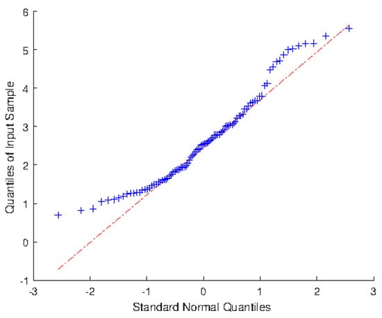
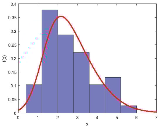
The above approaches are applied to the data of LAI of Robinia pseudoacacia Plantation in Huaiping Forest Farm, Yongshou County, Shanxi Province (see Ye et al. [42]). From Figure 1 and Figure 2, the distribution of LAI does not follow the normal distribution but shows asymmetric right-biased distribution characteristics. To confirm the conclusion, we first test the normality of this data. It turns out that the p-values from R output of Shapiro–Wilk test, Anderson–Darling test and Lilliefor test are 0.0007, 0.0014 and 0.0458, respectively. Hence, the LAI is not normally distributed at the nominal significance level of 5%. Further, we should prove whether the distribution of LAI is skew-normal by the Chi-square goodness-of-fit test. By calculation, we have . Therefore, the LAI follows the skew-normal distribution at the nominal significance level of 5%. Based on the method of moment estimation, the LAI is approximately distributed as , and its density curve is given in Figure 2.
Figure 1.
Q-Q plot of LAI data (Red line and blue line respectively denote the standard normal quantiles and sample quantiles).
Figure 2.
Frequency histogram of the LAI with superimposed skew-normal density curve.
To illustrate the proposed approach for hypothesis testing problem (19), we suppose as the nearby value of moment estimate of . Namely, consider the hypothesis testing problem:
Based on the moment and ML estimators, the p-values of Bootstrap test are 0.02584 and 0.00097, respectively. Hence, the null hypothesis is rejected at the nominal significance level of 5%, that is, the location parameter of LAI is not equal to 2 significantly.
Example 2.
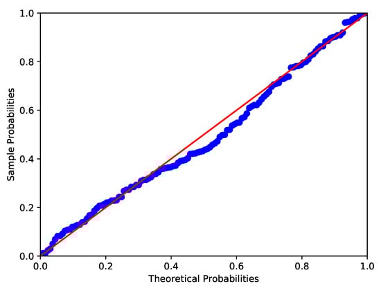
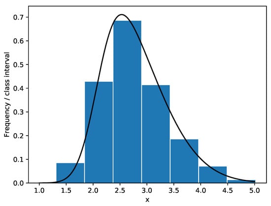
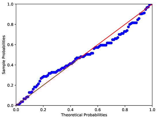
Kundu and Gupta [43] presented a data set of the strength measured in GPA for single carbon fibers. The Shapiro-Wilk test, Anderson-Darling test and Lilliefor test are used to test the normality of the data. It turns out that the p-values of the data are 0.0108, 0.0109 and 0.0254 respectively. The P-P plot and the histogram of the data are given in Figure 3 and Figure 4. Furthermore, the chi-square goodness-of-fit test is used to see whether the distribution of data is skew-normal, namely we set : the carbon fibers’ strength data is skew-normally distributed. We obtain that , then the null hypothesis is rejected at the nominal significance level of 5%. Similar to Example 1, the carbon fibers’ strength data is considered to follow skew normal distribution SN (2.0917, 0.9230, 2.9668).
Figure 3.
P-P plot of carbon fibers’ strength data (Red line and blue line respectively denote the theoretical probabilities and sample probabilities).
Figure 4.
Frequency histogram of the carbon fibers’ strength data with superimposed skew-normal density curve.
Consider the hypothesis testing problem:
By the moment and ML estimators, the p-values of Bootstrap test are 0.9433 and 0.0814, respectively. Therefore, the null hypothesis is not rejected at the nominal significance level of 5%.
Example 3.
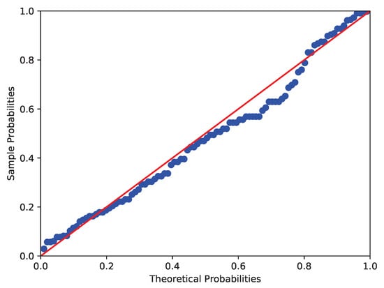
The data collected by the Australian Institute of Physical Education of RBC count in 102 male and 100 female athletes are analyzed in this example (see Cook and Weisberg [44]). Similar to Example 2, the Shapiro-Wilk test, Anderson-Darling test and Lilliefor test are used to test the normality of RBC count in male and female athletes. It shows that the p-values of RBC count in male athletes are 0.0000, 0.0019 and 0.0025 respectively, while those in female athletes are 0.0065, 0.0131 and 0.0181 respectively. The corresponding images are shown in Figure 5 and Figure 6. Therefore, at the nominal significance level of 5%, the above tests all reject the null hypothesis that RBC counts in male and female athletes follow normal distributions. Furthermore, to verify the skew-normality of RBC count, we test the null hypothesis : the RBC count is skew-normally distributed. It can be obtained by calculation that and , which means the RBC count in male and female athletes follow the skew-normal distributions and respectively at the nominal significance level of 5%.
Figure 5.
P-P plot of RBC count in male athletes (Red line and blue line respectively denote the theoretical probabilities and sample probabilities).
Figure 6.
P-P plot of RBC count in female athletes (Red line and blue line respectively denote the theoretical probabilities and sample probabilities).
Consider the hypothesis testing problem:
The p-values of Bootstrap test statistics based on the moment estimators and ML estimators are 0.00071 and 0.00153, respectively. Therefore, the null hypothesis is rejected at the nominal significance level of 5%, that is, the location parameters of RBC counts in male and female athletes have significant differences.
6. Conclusions
By using the centered parameterization and Bootstrap approaches, we study the hypothesis testing and interval estimation problems of location parameters for single and two skew-normal populations with unknown scale parameters and skewness parameters. Firstly, the Bootstrap test statistics and Bootstrap confidence intervals for location parameter of single population are constructed based on the moment estimators and ML estimators, respectively. Secondly, the Bootstrap approaches for Behrens-Fisher type and interval estimation problems are established for two skew-normal populations. Thirdly, the Monte Carlo simulation results show that the Bootstrap test based on the moment estimator is better than that based on the ML estimator in most parameter settings, whether in single population or two. Finally, the above approaches are applied to LAI, carbon fibers’ strength and RBC count in athletes to verify the rationality and validity of the proposed approaches. In summary, the Bootstrap approach based on the moment estimator is preferentially suggested to be used for inference on the location parameter of the skew-normal population. In the future, we plan to consider the hypothesis testing and confidence interval problems for the location parameter vector in multivariate skew-normal population, and discuss the applications of Bootstrap approach in multivariate skew-normal data sets, expecting to provide a feasible solution for the multivariate skew data analysis problem.
Author Contributions
Conceptualization, R.Y. and B.F.; methodology, R.Y. and B.F.; software, B.F.; validation, R.Y. and B.F.; formal analysis, R.Y. and B.F.; investigation, R.Y. and B.F.; data curation, B.F.; writing—original draft preparation, B.F., R.Y. and K.L.; writing—review and editing, R.Y., B.F., W.D., K.L. and Y.L.; supervision, R.Y.; funding acquisition, R.Y. All authors have read and agreed to the published version of the manuscript.
Funding
This work was supported by National Social Science Foundation of China (Grant No. 21BTJ068).
Institutional Review Board Statement
Not applicable.
Informed Consent Statement
Not applicable.
Data Availability Statement
The data that support the findings of this study are available on request from the corresponding author.
Conflicts of Interest
The authors declare no conflict of interest.
Appendix A

Table A1.
Simulated Type I error probabilities of hypothesis testing problem (19).
Table A1.
Simulated Type I error probabilities of hypothesis testing problem (19).
| p | |||||||||
|---|---|---|---|---|---|---|---|---|---|
| 4 | 0.0672 | 0.0544 | 0.0540 | 0.0528 | 0.0512 | 0.0480 | 0.0452 | 0.0484 | |
| 0.0608 | 0.0556 | 0.0484 | 0.0492 | 0.0464 | 0.0456 | 0.0404 | 0.0460 | ||
| 4.5 | 0.0588 | 0.0456 | 0.0460 | 0.0476 | 0.0440 | 0.0416 | 0.0424 | 0.0440 | |
| 0.0520 | 0.0504 | 0.0448 | 0.0428 | 0.0416 | 0.0440 | 0.0380 | 0.0420 | ||
| 5 | 0.0512 | 0.0396 | 0.0404 | 0.0408 | 0.0404 | 0.0368 | 0.0388 | 0.0412 | |
| 0.0472 | 0.0476 | 0.0408 | 0.0376 | 0.0404 | 0.0400 | 0.0352 | 0.0408 | ||
| 5.5 | 0.0480 | 0.0376 | 0.0376 | 0.0356 | 0.0380 | 0.0336 | 0.0380 | 0.0372 | |
| 0.0444 | 0.0416 | 0.0372 | 0.0356 | 0.0388 | 0.0380 | 0.0328 | 0.0396 | ||
| 6 | 0.0444 | 0.0356 | 0.0360 | 0.0344 | 0.0360 | 0.0316 | 0.0356 | 0.0352 | |
| 0.0428 | 0.0384 | 0.0344 | 0.0352 | 0.0368 | 0.0364 | 0.0304 | 0.0384 | ||
| 6.5 | 0.0420 | 0.0332 | 0.0328 | 0.0332 | 0.0348 | 0.0312 | 0.0348 | 0.0332 | |
| 0.0408 | 0.0364 | 0.0344 | 0.0324 | 0.0360 | 0.0352 | 0.0300 | 0.0360 | ||
| 7 | 0.0396 | 0.0324 | 0.0316 | 0.0316 | 0.0336 | 0.0296 | 0.0340 | 0.0324 | |
| 0.0388 | 0.0360 | 0.0332 | 0.0312 | 0.0356 | 0.0340 | 0.0288 | 0.0360 | ||
| 7.5 | 0.0364 | 0.0300 | 0.0304 | 0.0304 | 0.0332 | 0.0296 | 0.0320 | 0.0312 | |
| 0.0376 | 0.0360 | 0.0328 | 0.0312 | 0.0348 | 0.0332 | 0.0280 | 0.0356 | ||
| 8 | 0.0360 | 0.0288 | 0.0304 | 0.0296 | 0.0324 | 0.0288 | 0.0308 | 0.0308 | |
| 0.0360 | 0.0344 | 0.0328 | 0.0304 | 0.0340 | 0.0332 | 0.0272 | 0.0356 | ||
| −4 | 0.0680 | 0.0604 | 0.0596 | 0.0532 | 0.0528 | 0.0484 | 0.0488 | 0.0524 | |
| 0.0576 | 0.0604 | 0.0520 | 0.0484 | 0.0488 | 0.0460 | 0.0380 | 0.0460 | ||
| −4.5 | 0.0608 | 0.0524 | 0.0492 | 0.0456 | 0.0468 | 0.0448 | 0.0440 | 0.0464 | |
| 0.0512 | 0.0532 | 0.0444 | 0.0436 | 0.0424 | 0.0420 | 0.0356 | 0.0460 | ||
| −5 | 0.0540 | 0.0480 | 0.0448 | 0.0408 | 0.0428 | 0.0396 | 0.0424 | 0.0420 | |
| 0.0452 | 0.0472 | 0.0412 | 0.0404 | 0.0400 | 0.0388 | 0.0340 | 0.0428 | ||
| −5.5 | 0.0452 | 0.0452 | 0.0400 | 0.0376 | 0.0376 | 0.0372 | 0.0392 | 0.0392 | |
| 0.0400 | 0.0424 | 0.0388 | 0.0384 | 0.0396 | 0.0364 | 0.0312 | 0.0412 | ||
| −6 | 0.0412 | 0.0408 | 0.0368 | 0.0348 | 0.0352 | 0.0336 | 0.0376 | 0.0364 | |
| 0.0368 | 0.0416 | 0.0364 | 0.0364 | 0.0376 | 0.0360 | 0.0296 | 0.0400 | ||
| −6.5 | 0.0400 | 0.0376 | 0.0344 | 0.0320 | 0.0332 | 0.0328 | 0.0352 | 0.0340 | |
| 0.0344 | 0.0404 | 0.0356 | 0.0348 | 0.0364 | 0.0352 | 0.0284 | 0.0384 | ||
| −7 | 0.0372 | 0.0372 | 0.0324 | 0.0312 | 0.0328 | 0.0300 | 0.0340 | 0.0316 | |
| 0.0332 | 0.0400 | 0.0356 | 0.0328 | 0.0348 | 0.0348 | 0.0276 | 0.0368 | ||
| −7.5 | 0.0352 | 0.0364 | 0.0312 | 0.0308 | 0.0308 | 0.0292 | 0.0316 | 0.0308 | |
| 0.0320 | 0.0392 | 0.0344 | 0.0320 | 0.0344 | 0.0348 | 0.0272 | 0.0368 | ||
| −8 | 0.0344 | 0.0348 | 0.0312 | 0.0300 | 0.0296 | 0.0292 | 0.0304 | 0.0296 | |
| 0.0316 | 0.0380 | 0.0336 | 0.0308 | 0.0340 | 0.0344 | 0.0264 | 0.0360 |
Table A2.
Simulated powers of hypothesis testing problem (19) (positive skewness).
Table A2.
Simulated powers of hypothesis testing problem (19) (positive skewness).
| n | p | |||||||
|---|---|---|---|---|---|---|---|---|
| 1.9 | 1.8 | 1.7 | 1.6 | 1.5 | 1.4 | |||
| 4 | 40 | 0.1540 | 0.2936 | 0.4504 | 0.6184 | 0.7624 | 0.8556 | |
| 0.1288 | 0.2096 | 0.2684 | 0.3196 | 0.3700 | 0.4380 | |||
| 50 | 0.1776 | 0.3388 | 0.5076 | 0.7028 | 0.8280 | 0.9016 | ||
| 0.1368 | 0.2184 | 0.2860 | 0.3376 | 0.4060 | 0.4780 | |||
| 60 | 0.1700 | 0.3604 | 0.5636 | 0.7444 | 0.8740 | 0.9408 | ||
| 0.1372 | 0.2256 | 0.2832 | 0.3540 | 0.4288 | 0.5076 | |||
| 70 | 0.1848 | 0.3884 | 0.5968 | 0.7892 | 0.9000 | 0.9620 | ||
| 0.1348 | 0.2188 | 0.2872 | 0.3580 | 0.4416 | 0.5416 | |||
| 100 | 0.2052 | 0.4424 | 0.7096 | 0.8872 | 0.9616 | 0.9904 | ||
| 0.1376 | 0.2212 | 0.2980 | 0.3832 | 0.4892 | 0.5972 | |||
| 150 | 0.2636 | 0.5704 | 0.8376 | 0.9608 | 0.9924 | 0.9992 | ||
| 0.1532 | 0.2264 | 0.3012 | 0.4084 | 0.5324 | 0.6836 | |||
| 200 | 0.2988 | 0.6620 | 0.9156 | 0.9876 | 0.9980 | 1.0000 | ||
| 0.1472 | 0.2324 | 0.3348 | 0.4536 | 0.5960 | 0.7672 | |||
| 4.5 | 40 | 0.1476 | 0.2928 | 0.4580 | 0.6292 | 0.7836 | 0.8688 | |
| 0.1292 | 0.2188 | 0.2828 | 0.3404 | 0.3952 | 0.4632 | |||
| 50 | 0.1708 | 0.3452 | 0.5204 | 0.7164 | 0.8420 | 0.9136 | ||
| 0.1404 | 0.2396 | 0.3140 | 0.3632 | 0.4308 | 0.5092 | |||
| 60 | 0.1708 | 0.3656 | 0.5780 | 0.7644 | 0.8888 | 0.9484 | ||
| 0.1428 | 0.2380 | 0.3080 | 0.3836 | 0.4664 | 0.5456 | |||
| 70 | 0.1868 | 0.4004 | 0.6156 | 0.8016 | 0.9128 | 0.9660 | ||
| 0.1416 | 0.2452 | 0.3220 | 0.3956 | 0.4872 | 0.5816 | |||
| 100 | 0.2100 | 0.4640 | 0.7256 | 0.9024 | 0.9696 | 0.9932 | ||
| 0.1528 | 0.2496 | 0.3348 | 0.4284 | 0.5380 | 0.6452 | |||
| 150 | 0.2720 | 0.5928 | 0.8528 | 0.9684 | 0.9940 | 0.9996 | ||
| 0.1816 | 0.2644 | 0.3524 | 0.4660 | 0.5992 | 0.7288 | |||
| 200 | 0.3088 | 0.6828 | 0.9260 | 0.9908 | 0.9992 | 1.0000 | ||
| 0.1796 | 0.2804 | 0.3924 | 0.5108 | 0.6612 | 0.8100 | |||
| 5 | 40 | 0.1396 | 0.2944 | 0.4660 | 0.6404 | 0.7896 | 0.8768 | |
| 0.1284 | 0.2272 | 0.2992 | 0.3584 | 0.4180 | 0.4964 | |||
| 50 | 0.1668 | 0.3472 | 0.5332 | 0.7268 | 0.8556 | 0.9260 | ||
| 0.1400 | 0.2524 | 0.3300 | 0.3900 | 0.4568 | 0.5380 | |||
| 60 | 0.1700 | 0.3736 | 0.5868 | 0.7744 | 0.8948 | 0.9532 | ||
| 0.1468 | 0.2572 | 0.3348 | 0.4076 | 0.4908 | 0.5712 | |||
| 70 | 0.1844 | 0.4064 | 0.6288 | 0.8176 | 0.9256 | 0.9732 | ||
| 0.1476 | 0.2688 | 0.3504 | 0.4224 | 0.5156 | 0.6080 | |||
| 100 | 0.2140 | 0.4792 | 0.7396 | 0.9108 | 0.9756 | 0.9936 | ||
| 0.1620 | 0.2780 | 0.3724 | 0.4644 | 0.5720 | 0.6788 | |||
| 150 | 0.2780 | 0.6088 | 0.8624 | 0.9712 | 0.9956 | 1.0000 | ||
| 0.1992 | 0.2956 | 0.3916 | 0.5088 | 0.6416 | 0.7600 | |||
| 200 | 0.3208 | 0.6968 | 0.9340 | 0.9912 | 0.9992 | 1.0000 | ||
| 0.2104 | 0.3196 | 0.4316 | 0.5564 | 0.7104 | 0.8356 | |||
| 5.5 | 40 | 0.1372 | 0.2980 | 0.4732 | 0.6532 | 0.7972 | 0.8852 | |
| 0.1272 | 0.2328 | 0.3156 | 0.3732 | 0.4348 | 0.5136 | |||
| 50 | 0.1640 | 0.3540 | 0.5428 | 0.7436 | 0.8620 | 0.9348 | ||
| 0.1424 | 0.2608 | 0.3420 | 0.4084 | 0.4804 | 0.5568 | |||
| 60 | 0.1700 | 0.3800 | 0.5948 | 0.7848 | 0.9016 | 0.9604 | ||
| 0.1496 | 0.2688 | 0.3556 | 0.4312 | 0.5092 | 0.5988 | |||
| 70 | 0.1840 | 0.4136 | 0.6388 | 0.8252 | 0.9308 | 0.9752 | ||
| 0.1504 | 0.2864 | 0.3696 | 0.4456 | 0.5332 | 0.6268 | |||
| 100 | 0.2148 | 0.4904 | 0.7476 | 0.9192 | 0.9784 | 0.9952 | ||
| 0.1672 | 0.3032 | 0.3984 | 0.4952 | 0.6008 | 0.7016 | |||
| 150 | 0.2800 | 0.6220 | 0.8704 | 0.9744 | 0.9960 | 1.0000 | ||
| 0.2128 | 0.3180 | 0.4228 | 0.5452 | 0.6792 | 0.7908 | |||
| 200 | 0.3320 | 0.7148 | 0.9380 | 0.9924 | 0.9992 | 1.0000 | ||
| 0.2336 | 0.3496 | 0.4652 | 0.5932 | 0.7440 | 0.8540 | |||
| 6 | 40 | 0.1356 | 0.3008 | 0.4772 | 0.6628 | 0.8040 | 0.8892 | |
| 0.1236 | 0.2368 | 0.3236 | 0.3868 | 0.4472 | 0.5264 | |||
| 50 | 0.1620 | 0.3592 | 0.5496 | 0.7468 | 0.8688 | 0.9416 | ||
| 0.1416 | 0.2704 | 0.3560 | 0.4236 | 0.4964 | 0.5768 | |||
| 60 | 0.1700 | 0.3848 | 0.6040 | 0.7932 | 0.9072 | 0.9648 | ||
| 0.1492 | 0.2800 | 0.3676 | 0.4428 | 0.5216 | 0.6156 | |||
| 70 | 0.1840 | 0.4216 | 0.6488 | 0.8308 | 0.9364 | 0.9804 | ||
| 0.1532 | 0.2980 | 0.3848 | 0.4660 | 0.5500 | 0.6440 | |||
| 100 | 0.2140 | 0.4968 | 0.7572 | 0.9224 | 0.9824 | 0.9960 | ||
| 0.1688 | 0.3232 | 0.4184 | 0.5188 | 0.6208 | 0.7212 | |||
| 150 | 0.2816 | 0.6296 | 0.8784 | 0.9776 | 0.9964 | 1.0000 | ||
| 0.2240 | 0.3416 | 0.4496 | 0.5748 | 0.7048 | 0.8116 | |||
| 200 | 0.3416 | 0.7232 | 0.9420 | 0.9932 | 0.9996 | 1.0000 | ||
| 0.2524 | 0.3788 | 0.4932 | 0.6296 | 0.7732 | 0.8676 | |||
| 6.5 | 40 | 0.1336 | 0.3040 | 0.4816 | 0.6684 | 0.8100 | 0.8940 | |
| 0.1208 | 0.2400 | 0.3328 | 0.4008 | 0.4616 | 0.5392 | |||
| 50 | 0.1596 | 0.3628 | 0.5548 | 0.7528 | 0.8732 | 0.9448 | ||
| 0.1436 | 0.2764 | 0.3616 | 0.4312 | 0.5064 | 0.5896 | |||
| 60 | 0.1676 | 0.3900 | 0.6080 | 0.7992 | 0.9100 | 0.9680 | ||
| 0.1516 | 0.2916 | 0.3836 | 0.4584 | 0.5384 | 0.6308 | |||
| 70 | 0.1820 | 0.4264 | 0.6564 | 0.8348 | 0.9396 | 0.9828 | ||
| 0.1528 | 0.3052 | 0.3988 | 0.4780 | 0.5656 | 0.6596 | |||
| 100 | 0.2144 | 0.5048 | 0.7612 | 0.9256 | 0.9832 | 0.9960 | ||
| 0.1704 | 0.3364 | 0.4328 | 0.5360 | 0.6420 | 0.7320 | |||
| 150 | 0.2836 | 0.6368 | 0.8852 | 0.9784 | 0.9972 | 1.0000 | ||
| 0.2320 | 0.3588 | 0.4676 | 0.5972 | 0.7248 | 0.8232 | |||
| 200 | 0.3488 | 0.7296 | 0.9460 | 0.9944 | 0.9996 | 1.0000 | ||
| 0.2628 | 0.4016 | 0.5180 | 0.6572 | 0.7896 | 0.8840 | |||
| 7 | 40 | 0.1324 | 0.3052 | 0.4856 | 0.6740 | 0.8140 | 0.8984 | |
| 0.1184 | 0.2440 | 0.3400 | 0.4088 | 0.4692 | 0.5472 | |||
| 50 | 0.1588 | 0.3668 | 0.5608 | 0.7588 | 0.8756 | 0.9468 | ||
| 0.1432 | 0.2804 | 0.3704 | 0.4404 | 0.5148 | 0.6016 | |||
| 60 | 0.1676 | 0.3932 | 0.6144 | 0.8052 | 0.9116 | 0.9712 | ||
| 0.1512 | 0.3028 | 0.3928 | 0.4688 | 0.5496 | 0.6396 | |||
| 70 | 0.1800 | 0.4304 | 0.6616 | 0.8404 | 0.9420 | 0.9844 | ||
| 0.1528 | 0.3160 | 0.4072 | 0.4876 | 0.5800 | 0.6736 | |||
| 100 | 0.2168 | 0.5112 | 0.7652 | 0.9284 | 0.9836 | 0.9964 | ||
| 0.1708 | 0.3476 | 0.4432 | 0.5448 | 0.6520 | 0.7468 | |||
| 150 | 0.2856 | 0.6428 | 0.8868 | 0.9788 | 0.9976 | 1.0000 | ||
| 0.2352 | 0.3740 | 0.4860 | 0.6156 | 0.7416 | 0.8360 | |||
| 200 | 0.3512 | 0.7352 | 0.9496 | 0.9952 | 0.9996 | 1.0000 | ||
| 0.2760 | 0.4168 | 0.5324 | 0.6724 | 0.8032 | 0.8956 | |||
| 7.5 | 40 | 0.1304 | 0.3048 | 0.4876 | 0.6764 | 0.8176 | 0.9000 | |
| 0.1164 | 0.2484 | 0.3484 | 0.4148 | 0.4780 | 0.5560 | |||
| 50 | 0.1584 | 0.3680 | 0.5668 | 0.7632 | 0.8776 | 0.9492 | ||
| 0.1424 | 0.2856 | 0.3800 | 0.4500 | 0.5256 | 0.6136 | |||
| 60 | 0.1660 | 0.3968 | 0.6188 | 0.8100 | 0.9136 | 0.9740 | ||
| 0.1520 | 0.3084 | 0.3996 | 0.4756 | 0.5588 | 0.6500 | |||
| 70 | 0.1796 | 0.4344 | 0.6664 | 0.8448 | 0.9436 | 0.9848 | ||
| 0.1512 | 0.3212 | 0.4140 | 0.4960 | 0.5916 | 0.6844 | |||
| 100 | 0.2160 | 0.5152 | 0.7716 | 0.9288 | 0.9852 | 0.9964 | ||
| 0.1724 | 0.3572 | 0.4576 | 0.5556 | 0.6616 | 0.7572 | |||
| 150 | 0.2864 | 0.6484 | 0.8900 | 0.9792 | 0.9976 | 1.0000 | ||
| 0.2412 | 0.3856 | 0.5012 | 0.6308 | 0.7532 | 0.8456 | |||
| 200 | 0.3536 | 0.7388 | 0.9516 | 0.9956 | 0.9996 | 1.0000 | ||
| 0.2844 | 0.4288 | 0.5480 | 0.6864 | 0.8100 | 0.9016 | |||
| 8 | 40 | 0.1296 | 0.3064 | 0.4904 | 0.6808 | 0.8224 | 0.9024 | |
| 0.1148 | 0.2492 | 0.3500 | 0.4180 | 0.4848 | 0.5648 | |||
| 50 | 0.1580 | 0.3692 | 0.5684 | 0.7680 | 0.8836 | 0.9500 | ||
| 0.1424 | 0.2888 | 0.3848 | 0.4588 | 0.5340 | 0.6196 | |||
| 60 | 0.1648 | 0.4008 | 0.6228 | 0.8128 | 0.9164 | 0.9756 | ||
| 0.1512 | 0.3120 | 0.4052 | 0.4852 | 0.5660 | 0.6560 | |||
| 70 | 0.1792 | 0.4392 | 0.6724 | 0.8472 | 0.9456 | 0.9856 | ||
| 0.1520 | 0.3276 | 0.4216 | 0.5028 | 0.5996 | 0.6916 | |||
| 100 | 0.2152 | 0.5188 | 0.7752 | 0.9316 | 0.9856 | 0.9968 | ||
| 0.1728 | 0.3696 | 0.4672 | 0.5656 | 0.6680 | 0.7644 | |||
| 150 | 0.2872 | 0.6520 | 0.8972 | 0.9808 | 0.9976 | 1.0000 | ||
| 0.2444 | 0.3948 | 0.5108 | 0.6420 | 0.7592 | 0.8532 | |||
| 200 | 0.3564 | 0.7440 | 0.9532 | 0.9964 | 0.9996 | 1.0000 | ||
| 0.2896 | 0.4368 | 0.5616 | 0.6964 | 0.8192 | 0.9096 | |||
Table A3.
Simulated powers of hypothesis testing problem (19) (negative skewness).
Table A3.
Simulated powers of hypothesis testing problem (19) (negative skewness).
| n | p | |||||||
|---|---|---|---|---|---|---|---|---|
| 2.1 | 2.2 | 2.3 | 2.4 | 2.5 | 2.6 | |||
| −4 | 40 | 0.1592 | 0.2980 | 0.4600 | 0.6344 | 0.7696 | 0.8628 | |
| 0.1292 | 0.2100 | 0.2652 | 0.3060 | 0.3660 | 0.4392 | |||
| 50 | 0.1772 | 0.3344 | 0.5116 | 0.6992 | 0.8356 | 0.9100 | ||
| 0.1420 | 0.2268 | 0.2796 | 0.3336 | 0.3976 | 0.4832 | |||
| 60 | 0.1772 | 0.3588 | 0.5640 | 0.7472 | 0.8780 | 0.9404 | ||
| 0.1408 | 0.2244 | 0.2916 | 0.3524 | 0.4296 | 0.5120 | |||
| 70 | 0.1876 | 0.3884 | 0.6040 | 0.7920 | 0.9016 | 0.9620 | ||
| 0.1296 | 0.2188 | 0.2916 | 0.3680 | 0.4420 | 0.5280 | |||
| 100 | 0.2064 | 0.4460 | 0.6972 | 0.8764 | 0.9588 | 0.9908 | ||
| 0.1412 | 0.2256 | 0.2976 | 0.3824 | 0.4800 | 0.5872 | |||
| 150 | 0.2616 | 0.5700 | 0.8372 | 0.9648 | 0.9912 | 0.9992 | ||
| 0.1560 | 0.2312 | 0.3052 | 0.4188 | 0.5416 | 0.6828 | |||
| 200 | 0.2956 | 0.6496 | 0.9172 | 0.9888 | 0.9988 | 1.0000 | ||
| 0.1488 | 0.2356 | 0.3396 | 0.4508 | 0.5872 | 0.7512 | |||
| −4.5 | 40 | 0.1556 | 0.3000 | 0.4680 | 0.6464 | 0.7816 | 0.8756 | |
| 0.1264 | 0.2148 | 0.2820 | 0.3300 | 0.3960 | 0.4724 | |||
| 50 | 0.1704 | 0.3368 | 0.5216 | 0.7148 | 0.8464 | 0.9248 | ||
| 0.1404 | 0.2320 | 0.2968 | 0.3584 | 0.4340 | 0.5160 | |||
| 60 | 0.1744 | 0.3704 | 0.5808 | 0.7664 | 0.8952 | 0.9512 | ||
| 0.1440 | 0.2432 | 0.3144 | 0.3880 | 0.4712 | 0.5468 | |||
| 70 | 0.1884 | 0.4028 | 0.6244 | 0.8092 | 0.9144 | 0.9696 | ||
| 0.1364 | 0.2436 | 0.3248 | 0.4016 | 0.4792 | 0.5636 | |||
| 100 | 0.2132 | 0.4628 | 0.7212 | 0.8932 | 0.9676 | 0.9932 | ||
| 0.1520 | 0.2572 | 0.3352 | 0.4204 | 0.5248 | 0.6356 | |||
| 150 | 0.2692 | 0.5876 | 0.8536 | 0.9716 | 0.9936 | 0.9996 | ||
| 0.1832 | 0.2616 | 0.3580 | 0.4744 | 0.6000 | 0.7300 | |||
| 200 | 0.3084 | 0.6708 | 0.9268 | 0.9912 | 0.9996 | 1.0000 | ||
| 0.1820 | 0.2768 | 0.3916 | 0.5092 | 0.6524 | 0.8016 | |||
| −5 | 40 | 0.1504 | 0.2992 | 0.4728 | 0.6560 | 0.7960 | 0.8852 | |
| 0.1260 | 0.2268 | 0.3008 | 0.3500 | 0.4192 | 0.4972 | |||
| 50 | 0.1704 | 0.3444 | 0.5328 | 0.7280 | 0.8572 | 0.9336 | ||
| 0.1404 | 0.2444 | 0.3124 | 0.3784 | 0.4544 | 0.5452 | |||
| 60 | 0.1736 | 0.3804 | 0.5940 | 0.7792 | 0.9020 | 0.9564 | ||
| 0.1468 | 0.2600 | 0.3400 | 0.4148 | 0.4948 | 0.5752 | |||
| 70 | 0.1860 | 0.4136 | 0.6388 | 0.8188 | 0.9252 | 0.9752 | ||
| 0.1424 | 0.2684 | 0.3476 | 0.4308 | 0.5104 | 0.5932 | |||
| 100 | 0.2188 | 0.4764 | 0.7328 | 0.9020 | 0.9724 | 0.9944 | ||
| 0.1616 | 0.2836 | 0.3680 | 0.4608 | 0.5656 | 0.6712 | |||
| 150 | 0.2740 | 0.6004 | 0.8656 | 0.9732 | 0.9952 | 1.0000 | ||
| 0.1996 | 0.2940 | 0.3940 | 0.5164 | 0.6452 | 0.7640 | |||
| 200 | 0.3204 | 0.6924 | 0.9328 | 0.9932 | 0.9996 | 1.0000 | ||
| 0.2048 | 0.3160 | 0.4240 | 0.5572 | 0.7000 | 0.8288 | |||
| −5.5 | 40 | 0.1424 | 0.2972 | 0.4752 | 0.6588 | 0.8016 | 0.8896 | |
| 0.1220 | 0.2312 | 0.3096 | 0.3624 | 0.4352 | 0.5168 | |||
| 50 | 0.1668 | 0.3480 | 0.5400 | 0.7834 | 0.8680 | 0.9400 | ||
| 0.1436 | 0.2532 | 0.3288 | 0.3996 | 0.4732 | 0.5656 | |||
| 60 | 0.1700 | 0.3844 | 0.6012 | 0.7892 | 0.9060 | 0.9612 | ||
| 0.1476 | 0.2728 | 0.3584 | 0.4320 | 0.5152 | 0.5968 | |||
| 70 | 0.1864 | 0.4188 | 0.6464 | 0.8260 | 0.9316 | 0.9796 | ||
| 0.1460 | 0.2852 | 0.3660 | 0.4528 | 0.5288 | 0.6216 | |||
| 100 | 0.2208 | 0.4888 | 0.7416 | 0.9100 | 0.9756 | 0.9956 | ||
| 0.1676 | 0.3048 | 0.3940 | 0.4884 | 0.5924 | 0.6948 | |||
| 150 | 0.2796 | 0.6120 | 0.8748 | 0.9764 | 0.9956 | 1.0000 | ||
| 0.2148 | 0.3224 | 0.4244 | 0.5508 | 0.6772 | 0.7968 | |||
| 200 | 0.3300 | 0.7032 | 0.9372 | 0.9940 | 0.9996 | 1.0000 | ||
| 0.2308 | 0.3496 | 0.4568 | 0.5972 | 0.7336 | 0.8564 | |||
| −6 | 40 | 0.1388 | 0.3000 | 0.4816 | 0.6652 | 0.8080 | 0.8976 | |
| 0.1196 | 0.2384 | 0.3228 | 0.3748 | 0.4472 | 0.5296 | |||
| 50 | 0.1644 | 0.3544 | 0.5484 | 0.7492 | 0.8748 | 0.9440 | ||
| 0.1424 | 0.2576 | 0.3412 | 0.4160 | 0.4900 | 0.5832 | |||
| 60 | 0.1688 | 0.3892 | 0.6064 | 0.7956 | 0.9116 | 0.9660 | ||
| 0.1508 | 0.2856 | 0.3716 | 0.4456 | 0.5296 | 0.6168 | |||
| 70 | 0.1860 | 0.4220 | 0.6544 | 0.8328 | 0.9376 | 0.9808 | ||
| 0.1468 | 0.3020 | 0.3812 | 0.4688 | 0.5488 | 0.6436 | |||
| 100 | 0.2204 | 0.4964 | 0.7512 | 0.9140 | 0.9792 | 0.9960 | ||
| 0.1700 | 0.3236 | 0.4100 | 0.5088 | 0.6120 | 0.7160 | |||
| 150 | 0.2820 | 0.6252 | 0.8808 | 0.9784 | 0.9960 | 1.0000 | ||
| 0.2220 | 0.3420 | 0.4544 | 0.5756 | 0.7008 | 0.8148 | |||
| 200 | 0.3380 | 0.7160 | 0.9416 | 0.9940 | 0.9996 | 1.0000 | ||
| 0.2508 | 0.3732 | 0.4820 | 0.6264 | 0.7632 | 0.8748 | |||
| −6.5 | 40 | 0.1376 | 0.3024 | 0.4876 | 0.6708 | 0.8164 | 0.9032 | |
| 0.1188 | 0.2424 | 0.3296 | 0.3856 | 0.4560 | 0.5420 | |||
| 50 | 0.1620 | 0.3580 | 0.5528 | 0.7544 | 0.8800 | 0.9484 | ||
| 0.1432 | 0.2660 | 0.3504 | 0.4260 | 0.5044 | 0.5928 | |||
| 60 | 0.1672 | 0.3916 | 0.6104 | 0.7996 | 0.9164 | 0.9684 | ||
| 0.1524 | 0.2960 | 0.3832 | 0.4588 | 0.5432 | 0.6304 | |||
| 70 | 0.1848 | 0.4284 | 0.6600 | 0.8376 | 0.9412 | 0.9824 | ||
| 0.1492 | 0.3152 | 0.3928 | 0.4804 | 0.5620 | 0.6584 | |||
| 100 | 0.2188 | 0.5056 | 0.7612 | 0.9192 | 0.9808 | 0.9960 | ||
| 0.1704 | 0.3360 | 0.4284 | 0.5308 | 0.6268 | 0.7300 | |||
| 150 | 0.2832 | 0.6360 | 0.8876 | 0.9800 | 0.9972 | 1.0000 | ||
| 0.2312 | 0.3624 | 0.4720 | 0.5960 | 0.7172 | 0.8328 | |||
| 200 | 0.3444 | 0.7216 | 0.9440 | 0.9948 | 0.9996 | 1.0000 | ||
| 0.2660 | 0.3904 | 0.5040 | 0.6496 | 0.7820 | 0.8864 | |||
| −7 | 40 | 0.1348 | 0.3060 | 0.4896 | 0.6756 | 0.8220 | 0.9068 | |
| 0.1168 | 0.2436 | 0.3348 | 0.3964 | 0.4664 | 0.5520 | |||
| 50 | 0.1608 | 0.3600 | 0.5584 | 0.7600 | 0.8840 | 0.9524 | ||
| 0.1240 | 0.2460 | 0.3300 | 0.3940 | 0.4760 | 0.5680 | |||
| 60 | 0.1664 | 0.3952 | 0.6132 | 0.8044 | 0.9208 | 0.9704 | ||
| 0.1444 | 0.2728 | 0.3620 | 0.4384 | 0.5152 | 0.6056 | |||
| 70 | 0.1832 | 0.4308 | 0.6640 | 0.8408 | 0.9444 | 0.9828 | ||
| 0.1516 | 0.3244 | 0.4016 | 0.4912 | 0.5724 | 0.6728 | |||
| 100 | 0.2160 | 0.5100 | 0.7688 | 0.9232 | 0.9816 | 0.9964 | ||
| 0.1700 | 0.3472 | 0.4424 | 0.5416 | 0.6424 | 0.7448 | |||
| 150 | 0.2836 | 0.6416 | 0.8908 | 0.9812 | 0.9976 | 1.0000 | ||
| 0.2368 | 0.3788 | 0.4884 | 0.6140 | 0.7396 | 0.8404 | |||
| 200 | 0.3496 | 0.7300 | 0.9472 | 0.9960 | 0.9996 | 1.0000 | ||
| 0.2728 | 0.4068 | 0.5256 | 0.6696 | 0.7960 | 0.8952 | |||
| −7.5 | 40 | 0.1308 | 0.3056 | 0.4924 | 0.6776 | 0.8260 | 0.9100 | |
| 0.1136 | 0.2460 | 0.3384 | 0.4044 | 0.4748 | 0.5576 | |||
| 50 | 0.1604 | 0.3628 | 0.5624 | 0.7628 | 0.8860 | 0.9528 | ||
| 0.1448 | 0.2812 | 0.3732 | 0.4448 | 0.5212 | 0.6160 | |||
| 60 | 0.1644 | 0.3956 | 0.6180 | 0.8076 | 0.9212 | 0.9728 | ||
| 0.1516 | 0.3112 | 0.3992 | 0.4740 | 0.5604 | 0.6492 | |||
| 70 | 0.1816 | 0.4368 | 0.6700 | 0.8460 | 0.9464 | 0.9848 | ||
| 0.1524 | 0.3284 | 0.4132 | 0.5008 | 0.5844 | 0.6816 | |||
| 100 | 0.2152 | 0.5152 | 0.7740 | 0.9280 | 0.9824 | 0.9964 | ||
| 0.1716 | 0.3552 | 0.4540 | 0.5500 | 0.6540 | 0.7568 | |||
| 150 | 0.2852 | 0.6460 | 0.8932 | 0.9824 | 0.9976 | 1.0000 | ||
| 0.2420 | 0.3880 | 0.5052 | 0.6256 | 0.7488 | 0.8488 | |||
| 200 | 0.3528 | 0.7360 | 0.9504 | 0.9964 | 0.9996 | 1.0000 | ||
| 0.2808 | 0.4200 | 0.5444 | 0.6860 | 0.8076 | 0.9000 | |||
| −8 | 40 | 0.1300 | 0.3072 | 0.4952 | 0.6808 | 0.8288 | 0.9116 | |
| 0.1124 | 0.2476 | 0.3432 | 0.4108 | 0.4808 | 0.5624 | |||
| 50 | 0.1592 | 0.3652 | 0.5656 | 0.7648 | 0.8908 | 0.9552 | ||
| 0.1444 | 0.2856 | 0.3772 | 0.4508 | 0.5292 | 0.6252 | |||
| 60 | 0.1648 | 0.3984 | 0.6236 | 0.8092 | 0.9224 | 0.9732 | ||
| 0.1524 | 0.3176 | 0.4012 | 0.4784 | 0.5672 | 0.6592 | |||
| 70 | 0.1808 | 0.4388 | 0.6748 | 0.8476 | 0.9472 | 0.9848 | ||
| 0.1524 | 0.3320 | 0.4216 | 0.5080 | 0.5948 | 0.6884 | |||
| 100 | 0.2148 | 0.5188 | 0.7784 | 0.9292 | 0.9824 | 0.9968 | ||
| 0.1728 | 0.3604 | 0.4652 | 0.5588 | 0.6676 | 0.7652 | |||
| 150 | 0.2856 | 0.6496 | 0.8968 | 0.9828 | 0.9984 | 1.0000 | ||
| 0.2440 | 0.3988 | 0.5180 | 0.6384 | 0.7620 | 0.8576 | |||
| 200 | 0.3580 | 0.7392 | 0.9508 | 0.9968 | 0.9996 | 1.0000 | ||
| 0.2892 | 0.4296 | 0.5588 | 0.6984 | 0.8148 | 0.9072 | |||
Table A4.
Simulated Type I error probabilities of hypothesis testing problem (27).
Table A4.
Simulated Type I error probabilities of hypothesis testing problem (27).
| 40 | 50 | 0.1 | 0.3 | 0.0656 | 0.0676 | 0.0516 | 0.0428 |
| 0.2 | 0.5 | 0.0688 | 0.0516 | 0.0508 | 0.0268 | ||
| 0.3 | 0.7 | 0.0684 | 0.0484 | 0.0512 | 0.0244 | ||
| 0.4 | 0.9 | 0.0680 | 0.0476 | 0.0516 | 0.0244 | ||
| 0.5 | 1.0 | 0.0652 | 0.0392 | 0.0472 | 0.0208 | ||
| 50 | 50 | 0.1 | 0.3 | 0.0652 | 0.0760 | 0.0484 | 0.0528 |
| 0.2 | 0.5 | 0.0628 | 0.0540 | 0.0504 | 0.0312 | ||
| 0.3 | 0.7 | 0.0612 | 0.0408 | 0.0504 | 0.0232 | ||
| 0.4 | 0.9 | 0.0600 | 0.0348 | 0.0484 | 0.0188 | ||
| 0.5 | 1.0 | 0.0540 | 0.0264 | 0.0440 | 0.0132 | ||
| 50 | 60 | 0.1 | 0.3 | 0.0596 | 0.0576 | 0.0456 | 0.0520 |
| 0.2 | 0.5 | 0.0580 | 0.0416 | 0.0460 | 0.0236 | ||
| 0.3 | 0.7 | 0.0564 | 0.0352 | 0.0448 | 0.0180 | ||
| 0.4 | 0.9 | 0.0552 | 0.0304 | 0.0448 | 0.0168 | ||
| 0.5 | 1.0 | 0.0500 | 0.0236 | 0.0376 | 0.0096 | ||
| 60 | 70 | 0.1 | 0.3 | 0.0592 | 0.0492 | 0.0464 | 0.0548 |
| 0.2 | 0.5 | 0.0536 | 0.0356 | 0.0452 | 0.0300 | ||
| 0.3 | 0.7 | 0.0508 | 0.0324 | 0.0448 | 0.0232 | ||
| 0.4 | 0.9 | 0.0492 | 0.0300 | 0.0432 | 0.0184 | ||
| 0.5 | 1.0 | 0.0444 | 0.0220 | 0.0372 | 0.0112 | ||
| 70 | 80 | 0.1 | 0.3 | 0.0576 | 0.0452 | 0.0488 | 0.0444 |
| 0.2 | 0.5 | 0.0528 | 0.0324 | 0.0464 | 0.0332 | ||
| 0.3 | 0.7 | 0.0512 | 0.0272 | 0.0448 | 0.0288 | ||
| 0.4 | 0.9 | 0.0504 | 0.0224 | 0.0444 | 0.0260 | ||
| 0.5 | 1.0 | 0.0404 | 0.0184 | 0.0396 | 0.0168 | ||
| 80 | 90 | 0.1 | 0.3 | 0.0512 | 0.0456 | 0.0440 | 0.0732 |
| 0.2 | 0.5 | 0.0468 | 0.0332 | 0.0432 | 0.0532 | ||
| 0.3 | 0.7 | 0.0456 | 0.0280 | 0.0416 | 0.0428 | ||
| 0.4 | 0.9 | 0.0452 | 0.0284 | 0.0416 | 0.0372 | ||
| 0.5 | 1.0 | 0.0404 | 0.0232 | 0.0380 | 0.0256 | ||
| 90 | 120 | 0.1 | 0.3 | 0.0584 | 0.0300 | 0.0476 | 0.0460 |
| 0.2 | 0.5 | 0.0540 | 0.0364 | 0.0496 | 0.0428 | ||
| 0.3 | 0.7 | 0.0508 | 0.0248 | 0.0480 | 0.0404 | ||
| 0.4 | 0.9 | 0.0492 | 0.0272 | 0.0464 | 0.0320 | ||
| 0.5 | 1.0 | 0.0436 | 0.0208 | 0.0420 | 0.0232 | ||
| 120 | 150 | 0.1 | 0.3 | 0.0576 | 0.0216 | 0.0460 | 0.0496 |
| 0.2 | 0.5 | 0.0556 | 0.0220 | 0.0480 | 0.0496 | ||
| 0.3 | 0.7 | 0.0560 | 0.0164 | 0.0472 | 0.0444 | ||
| 0.4 | 0.9 | 0.0552 | 0.0220 | 0.0472 | 0.0408 | ||
| 0.5 | 1.0 | 0.0504 | 0.0172 | 0.0472 | 0.0312 | ||
| 150 | 200 | 0.1 | 0.3 | 0.0548 | 0.0188 | 0.0448 | 0.0384 |
| 0.2 | 0.5 | 0.0552 | 0.0192 | 0.0488 | 0.0340 | ||
| 0.3 | 0.7 | 0.0552 | 0.0160 | 0.0476 | 0.0348 | ||
| 0.4 | 0.9 | 0.0548 | 0.0168 | 0.0480 | 0.0368 | ||
| 0.5 | 1.0 | 0.0512 | 0.0192 | 0.0484 | 0.0372 | ||
Table A5.
Simulated powers of hypothesis testing problem (27) .
Table A5.
Simulated powers of hypothesis testing problem (27) .
| p | |||||||||
|---|---|---|---|---|---|---|---|---|---|
| 0.1 | 0.15 | 0.2 | 0.25 | 0.3 | |||||
| 40 | 50 | 0.1 | 0.3 | 0.5820 | 0.8376 | 0.9460 | 0.9820 | 0.9892 | |
| 0.5736 | 0.8284 | 0.9388 | 0.9736 | 0.9800 | |||||
| 0.2 | 0.5 | 0.3244 | 0.4960 | 0.6628 | 0.8068 | 0.8948 | |||
| 0.2172 | 0.3604 | 0.5488 | 0.7092 | 0.8320 | |||||
| 0.3 | 0.7 | 0.2196 | 0.3356 | 0.4552 | 0.5672 | 0.6876 | |||
| 0.1248 | 0.1972 | 0.2812 | 0.3952 | 0.5200 | |||||
| 0.4 | 0.9 | 0.1696 | 0.2504 | 0.3384 | 0.4272 | 0.5192 | |||
| 0.0900 | 0.1328 | 0.1848 | 0.2424 | 0.3232 | |||||
| 0.5 | 1.0 | 0.1316 | 0.1912 | 0.2612 | 0.3456 | 0.4188 | |||
| 0.0652 | 0.0848 | 0.1100 | 0.1488 | 0.1956 | |||||
| 50 | 50 | 0.1 | 0.3 | 0.6068 | 0.8288 | 0.9440 | 0.9812 | 0.9888 | |
| 0.6408 | 0.8696 | 0.9492 | 0.9744 | 0.9840 | |||||
| 0.2 | 0.5 | 0.3308 | 0.5288 | 0.6900 | 0.8112 | 0.9004 | |||
| 0.2740 | 0.4744 | 0.6692 | 0.8092 | 0.9040 | |||||
| 0.3 | 0.7 | 0.2264 | 0.3472 | 0.4912 | 0.6060 | 0.7228 | |||
| 0.1492 | 0.2508 | 0.3900 | 0.5272 | 0.6608 | |||||
| 0.4 | 0.9 | 0.1780 | 0.2528 | 0.3532 | 0.4660 | 0.5568 | |||
| 0.1108 | 0.1580 | 0.2372 | 0.3392 | 0.4480 | |||||
| 0.5 | 1.0 | 0.1428 | 0.2092 | 0.2764 | 0.3672 | 0.4616 | |||
| 0.0636 | 0.0992 | 0.1364 | 0.1968 | 0.2672 | |||||
| 50 | 60 | 0.1 | 0.3 | 0.6376 | 0.8716 | 0.9632 | 0.9876 | 0.9944 | |
| 0.6388 | 0.8752 | 0.9624 | 0.9836 | 0.9888 | |||||
| 0.2 | 0.5 | 0.3440 | 0.5480 | 0.7220 | 0.8540 | 0.9276 | |||
| 0.2736 | 0.4784 | 0.6812 | 0.8352 | 0.9184 | |||||
| 0.3 | 0.7 | 0.2252 | 0.3552 | 0.4988 | 0.6328 | 0.7476 | |||
| 0.1300 | 0.2536 | 0.3900 | 0.5264 | 0.6448 | |||||
| 0.4 | 0.9 | 0.1748 | 0.2560 | 0.3624 | 0.4712 | 0.5800 | |||
| 0.0944 | 0.1432 | 0.2456 | 0.3484 | 0.4496 | |||||
| 0.5 | 1.0 | 0.1416 | 0.2024 | 0.2800 | 0.3732 | 0.4696 | |||
| 0.0524 | 0.0820 | 0.1216 | 0.1808 | 0.2640 | |||||
| 60 | 70 | 0.1 | 0.3 | 0.6508 | 0.9000 | 0.9764 | 0.9940 | 0.9972 | |
| 0.6540 | 0.9172 | 0.9752 | 0.9896 | 0.9952 | |||||
| 0.2 | 0.5 | 0.3588 | 0.5568 | 0.7412 | 0.8804 | 0.9480 | |||
| 0.2812 | 0.5208 | 0.7492 | 0.8936 | 0.9504 | |||||
| 0.3 | 0.7 | 0.2416 | 0.3720 | 0.5164 | 0.6464 | 0.7752 | |||
| 0.1504 | 0.2748 | 0.4400 | 0.6124 | 0.7692 | |||||
| 0.4 | 0.9 | 0.1844 | 0.2748 | 0.3796 | 0.4932 | 0.5960 | |||
| 0.0852 | 0.1576 | 0.2616 | 0.3920 | 0.5208 | |||||
| 0.5 | 1.0 | 0.1360 | 0.2156 | 0.3052 | 0.3996 | 0.4908 | |||
| 0.0532 | 0.0840 | 0.1448 | 0.2292 | 0.3308 | |||||
| 70 | 80 | 0.1 | 0.3 | 0.7184 | 0.9324 | 0.9896 | 0.9976 | 0.9992 | |
| 0.7136 | 0.9356 | 0.9864 | 0.9948 | 0.9972 | |||||
| 0.2 | 0.5 | 0.4024 | 0.6232 | 0.8060 | 0.9232 | 0.9680 | |||
| 0.3084 | 0.5796 | 0.8160 | 0.9236 | 0.9712 | |||||
| 0.3 | 0.7 | 0.2664 | 0.4252 | 0.5740 | 0.7212 | 0.8368 | |||
| 0.1684 | 0.3108 | 0.5108 | 0.6968 | 0.8304 | |||||
| 0.4 | 0.9 | 0.1932 | 0.3120 | 0.4356 | 0.5440 | 0.6712 | |||
| 0.1092 | 0.1996 | 0.3216 | 0.4580 | 0.6220 | |||||
| 0.5 | 1.0 | 0.1596 | 0.2432 | 0.3460 | 0.4520 | 0.5552 | |||
| 0.0700 | 0.1256 | 0.1980 | 0.3036 | 0.4316 | |||||
| 80 | 90 | 0.1 | 0.3 | 0.7520 | 0.9484 | 0.9952 | 1.0000 | 1.0000 | |
| 0.7336 | 0.9496 | 0.9888 | 0.9980 | 1.0000 | |||||
| 0.2 | 0.5 | 0.4080 | 0.6536 | 0.8400 | 0.9392 | 0.9784 | |||
| 0.3272 | 0.6064 | 0.8412 | 0.9416 | 0.9756 | |||||
| 0.3 | 0.7 | 0.2548 | 0.4280 | 0.6060 | 0.7592 | 0.8684 | |||
| 0.1760 | 0.3352 | 0.5372 | 0.7252 | 0.8680 | |||||
| 0.4 | 0.9 | 0.1872 | 0.3004 | 0.4356 | 0.5808 | 0.6992 | |||
| 0.1764 | 0.2136 | 0.3460 | 0.4980 | 0.6480 | |||||
| 0.5 | 1.0 | 0.1464 | 0.2412 | 0.3496 | 0.4740 | 0.5940 | |||
| 0.0672 | 0.1232 | 0.2172 | 0.3336 | 0.4740 | |||||
| 90 | 120 | 0.1 | 0.3 | 0.8372 | 0.9796 | 0.9992 | 1.0000 | 1.0000 | |
| 0.7480 | 0.9716 | 0.9988 | 0.9996 | 0.9996 | |||||
| 0.2 | 0.5 | 0.4680 | 0.7372 | 0.9164 | 0.9704 | 0.9948 | |||
| 0.2884 | 0.6076 | 0.8640 | 0.9652 | 0.9952 | |||||
| 0.3 | 0.7 | 0.3152 | 0.4984 | 0.6868 | 0.8500 | 0.9320 | |||
| 0.1416 | 0.3012 | 0.5368 | 0.7560 | 0.8960 | |||||
| 0.4 | 0.9 | 0.2396 | 0.3660 | 0.5124 | 0.6632 | 0.7924 | |||
| 0.0956 | 0.1804 | 0.3140 | 0.4944 | 0.6756 | |||||
| 0.5 | 1.0 | 0.1876 | 0.3004 | 0.4164 | 0.5592 | 0.6856 | |||
| 0.0660 | 0.1172 | 0.2052 | 0.3488 | 0.5124 | |||||
| 120 | 150 | 0.1 | 0.3 | 0.9024 | 0.9972 | 0.9996 | 1.0000 | 1.0000 | |
| 0.7836 | 0.9960 | 0.9996 | 1.0000 | 1.0000 | |||||
| 0.2 | 0.5 | 0.5652 | 0.8260 | 0.9600 | 0.9948 | 0.9988 | |||
| 0.3008 | 0.6672 | 0.9204 | 0.9904 | 0.9988 | |||||
| 0.3 | 0.7 | 0.3780 | 0.6032 | 0.7880 | 0.9180 | 0.9732 | |||
| 0.1424 | 0.3564 | 0.6252 | 0.8408 | 0.9516 | |||||
| 0.4 | 0.9 | 0.2708 | 0.4440 | 0.6204 | 0.7596 | 0.8740 | |||
| 0.0980 | 0.1996 | 0.3820 | 0.5836 | 0.7728 | |||||
| 0.5 | 1.0 | 0.2244 | 0.3668 | 0.5196 | 0.6680 | 0.7912 | |||
| 0.0656 | 0.1368 | 0.2684 | 0.4480 | 0.6396 | |||||
Table A6.
Simulated powers of hypothesis testing problem (27) .
Table A6.
Simulated powers of hypothesis testing problem (27) .
| p | |||||||||
|---|---|---|---|---|---|---|---|---|---|
| 0.1 | 0.15 | 0.2 | 0.25 | 0.3 | |||||
| 40 | 50 | 0.1 | 0.3 | 0.6188 | 0.8600 | 0.9620 | 0.9896 | 0.9964 | |
| 0.7100 | 0.9144 | 0.9752 | 0.9884 | 0.9904 | |||||
| 0.2 | 0.5 | 0.3324 | 0.5268 | 0.7068 | 0.8412 | 0.9180 | |||
| 0.2448 | 0.4528 | 0.6628 | 0.8176 | 0.9112 | |||||
| 0.3 | 0.7 | 0.2196 | 0.3468 | 0.4872 | 0.6092 | 0.7296 | |||
| 0.1136 | 0.2100 | 0.3400 | 0.4896 | 0.6348 | |||||
| 0.4 | 0.9 | 0.1596 | 0.2528 | 0.3536 | 0.4624 | 0.5536 | |||
| 0.0676 | 0.1208 | 0.1964 | 0.2856 | 0.3952 | |||||
| 0.5 | 1.0 | 0.1248 | 0.1932 | 0.2724 | 0.3664 | 0.4584 | |||
| 0.0404 | 0.0592 | 0.0932 | 0.1380 | 0.2008 | |||||
| 50 | 50 | 0.1 | 0.3 | 0.6444 | 0.8628 | 0.9608 | 0.9880 | 0.9940 | |
| 0.7884 | 0.9400 | 0.9808 | 0.9888 | 0.9920 | |||||
| 0.2 | 0.5 | 0.3508 | 0.5596 | 0.7280 | 0.8484 | 0.9268 | |||
| 0.3448 | 0.5892 | 0.7932 | 0.9048 | 0.9584 | |||||
| 0.3 | 0.7 | 0.2348 | 0.3664 | 0.5244 | 0.6492 | 0.7556 | |||
| 0.1620 | 0.3028 | 0.4652 | 0.6416 | 0.7752 | |||||
| 0.4 | 0.9 | 0.1776 | 0.2672 | 0.3780 | 0.5012 | 0.5980 | |||
| 0.1008 | 0.1732 | 0.2756 | 0.4016 | 0.5256 | |||||
| 0.5 | 1.0 | 0.1428 | 0.2184 | 0.2984 | 0.4032 | 0.5044 | |||
| 0.0472 | 0.0824 | 0.1360 | 0.2008 | 0.2908 | |||||
| 50 | 60 | 0.1 | 0.3 | 0.6864 | 0.9016 | 0.9768 | 0.9940 | 0.9988 | |
| 0.8100 | 0.9608 | 0.9872 | 0.9936 | 0.9948 | |||||
| 0.2 | 0.5 | 0.3732 | 0.5852 | 0.7628 | 0.8864 | 0.9500 | |||
| 0.3456 | 0.6116 | 0.8260 | 0.9324 | 0.9712 | |||||
| 0.3 | 0.7 | 0.2372 | 0.3876 | 0.5420 | 0.6864 | 0.7920 | |||
| 0.1556 | 0.3040 | 0.4908 | 0.7104 | 0.8064 | |||||
| 0.4 | 0.9 | 0.1748 | 0.2712 | 0.3972 | 0.5136 | 0.6288 | |||
| 0.0848 | 0.1748 | 0.2820 | 0.4216 | 0.5576 | |||||
| 0.5 | 1.0 | 0.1384 | 0.2164 | 0.3128 | 0.4144 | 0.5192 | |||
| 0.0384 | 0.0756 | 0.1280 | 0.2028 | 0.2992 | |||||
| 60 | 70 | 0.1 | 0.3 | 0.6956 | 0.9256 | 0.9880 | 0.9972 | 0.9992 | |
| 0.8476 | 0.9692 | 0.9928 | 0.9960 | 0.9984 | |||||
| 0.2 | 0.5 | 0.3976 | 0.6040 | 0.7916 | 0.9120 | 0.9652 | |||
| 0.4684 | 0.7404 | 0.9084 | 0.9648 | 0.9824 | |||||
| 0.3 | 0.7 | 0.2560 | 0.4144 | 0.5640 | 0.7060 | 0.8260 | |||
| 0.2464 | 0.4588 | 0.6588 | 0.8164 | 0.9180 | |||||
| 0.4 | 0.9 | 0.1868 | 0.2980 | 0.4220 | 0.5368 | 0.6472 | |||
| 0.1444 | 0.2760 | 0.4452 | 0.6084 | 0.7352 | |||||
| 0.5 | 1.0 | 0.1460 | 0.2356 | 0.3376 | 0.4476 | 0.5512 | |||
| 0.0680 | 0.1448 | 0.2520 | 0.3924 | 0.5268 | |||||
| 70 | 80 | 0.1 | 0.3 | 0.7588 | 0.9536 | 0.9960 | 0.9996 | 1.0000 | |
| 0.8728 | 0.9800 | 0.9948 | 0.9984 | 0.9992 | |||||
| 0.2 | 0.5 | 0.4408 | 0.6696 | 0.8464 | 0.9452 | 0.9844 | |||
| 0.5476 | 0.7940 | 0.9300 | 0.9784 | 0.9912 | |||||
| 0.3 | 0.7 | 0.2908 | 0.4616 | 0.6248 | 0.7720 | 0.8788 | |||
| 0.3336 | 0.5676 | 0.7500 | 0.8776 | 0.9460 | |||||
| 0.4 | 0.9 | 0.2096 | 0.3424 | 0.4740 | 0.6020 | 0.7228 | |||
| 0.2252 | 0.4000 | 0.5768 | 0.7200 | 0.8344 | |||||
| 0.5 | 1.0 | 0.1672 | 0.2756 | 0.3932 | 0.5044 | 0.6140 | |||
| 0.1328 | 0.2616 | 0.4100 | 0.5716 | 0.7064 | |||||
| 80 | 90 | 0.1 | 0.3 | 0.7948 | 0.9676 | 0.9976 | 1.0000 | 1.0000 | |
| 0.8956 | 0.9876 | 0.9996 | 1.0000 | 1.0000 | |||||
| 0.2 | 0.5 | 0.4520 | 0.7000 | 0.8764 | 0.9588 | 0.9896 | |||
| 0.5752 | 0.8188 | 0.9456 | 0.9852 | 0.9964 | |||||
| 0.3 | 0.7 | 0.2804 | 0.4768 | 0.6552 | 0.8060 | 0.9012 | |||
| 0.3608 | 0.5980 | 0.7816 | 0.8988 | 0.9596 | |||||
| 0.4 | 0.9 | 0.1992 | 0.3412 | 0.4888 | 0.6288 | 0.7528 | |||
| 0.2500 | 0.4220 | 0.6048 | 0.7584 | 0.8608 | |||||
| 0.5 | 1.0 | 0.1604 | 0.2652 | 0.4056 | 0.5360 | 0.6552 | |||
| 0.1696 | 0.3040 | 0.4660 | 0.6304 | 0.7684 | |||||
| 90 | 120 | 0.1 | 0.3 | 0.8720 | 0.9888 | 1.0000 | 1.0000 | 1.0000 | |
| 0.9152 | 0.9932 | 1.0000 | 1.0000 | 1.0000 | |||||
| 0.2 | 0.5 | 0.5252 | 0.7896 | 0.9372 | 0.9852 | 0.9992 | |||
| 0.5560 | 0.8352 | 0.9652 | 0.9932 | 0.9992 | |||||
| 0.3 | 0.7 | 0.3468 | 0.5560 | 0.7432 | 0.8864 | 0.9500 | |||
| 0.3412 | 0.5916 | 0.7936 | 0.9248 | 0.9764 | |||||
| 0.4 | 0.9 | 0.2616 | 0.3992 | 0.5748 | 0.7156 | 0.8440 | |||
| 0.2404 | 0.4196 | 0.6148 | 0.7612 | 0.8808 | |||||
| 0.5 | 1.0 | 0.2068 | 0.3400 | 0.4756 | 0.6268 | 0.7424 | |||
| 0.1680 | 0.3164 | 0.4988 | 0.6672 | 0.8004 | |||||
| 120 | 150 | 0.1 | 0.3 | 0.9300 | 0.9976 | 1.0000 | 1.0000 | 1.0000 | |
| 0.9552 | 0.9984 | 1.0000 | 1.0000 | 1.0000 | |||||
| 0.2 | 0.5 | 0.6220 | 0.8628 | 0.9748 | 0.9972 | 0.9988 | |||
| 0.5948 | 0.9008 | 0.9852 | 0.9992 | 0.9996 | |||||
| 0.3 | 0.7 | 0.4180 | 0.6512 | 0.8304 | 0.9444 | 0.9864 | |||
| 0.3656 | 0.6460 | 0.8808 | 0.9676 | 0.9924 | |||||
| 0.4 | 0.9 | 0.3008 | 0.4964 | 0.6636 | 0.8060 | 0.9088 | |||
| 0.2476 | 0.4532 | 0.6760 | 0.8544 | 0.9492 | |||||
| 0.5 | 1.0 | 0.2564 | 0.4144 | 0.5832 | 0.7260 | 0.8368 | |||
| 0.2032 | 0.3680 | 0.5736 | 0.7588 | 0.8916 | |||||
References
- Ghosh, P.; Bayes, C.L.; Lachos, V.H. A robust Bayesian approach to null intercept measurement error model with application to dental data. Comput. Stat. Data Anal. 2009, 53, 1066–1079. [Google Scholar] [CrossRef]
- Zou, Y.J.; Zhang, Y.L. Use of skew-normal and skew-t distributions for mixture modeling of freeway speed data. Transport. Res. Rec. 2011, 2260, 67–75. [Google Scholar] [CrossRef]
- Li, C.I.; Su, N.C.; Su, P.F. The Design of and R Control Charts for Skew Normal Distributed Data. Commun. Statist. Theory Meth. 2014, 43, 4908–4924. [Google Scholar] [CrossRef]
- Azzalini, A. A class of distribution which includes the normal ones. Scand. J. Statist. 1985, 12, 171–178. [Google Scholar]
- Azzalini, A. Further results on a class of distributions which includes the normal ones. Statistica 1986, 49, 199–208. [Google Scholar]
- Arnold, B.C.; Lin, G.D. Characterizations of the skew-normal and generalized chi distributions. Sankhya 2004, 66, 593–606. [Google Scholar]
- Gupta, A.K.; Nguyen, T.T.; Sanqui, J.A.T. Characterization of the skew-normal distribution. Ann. Inst. Statist. Math. 2004, 56, 351–360. [Google Scholar] [CrossRef]
- Kim, H.M.; Genton, M.G. Characteristic functions of scale mixtures of multivariate skew-normal distributions. J. Multivar. Anal. 2011, 102, 1105–1117. [Google Scholar] [CrossRef]
- Su, N.C.; Gupta, A.K. On some sampling distributions for skew-normal population. J. Stat. Comput. Simul. 2015, 85, 3549–3559. [Google Scholar] [CrossRef]
- Gupta, A.K.; Huang, W.J. Quadratic forms in skew normal variates. J. Math. Anal. Appl. 2002, 273, 558–564. [Google Scholar] [CrossRef][Green Version]
- Wang, T.H.; Li, B.K.; Gupta, A.K. Distribution of quadratic forms under skew normal settings. J. Multivar. Anal. 2009, 100, 533–545. [Google Scholar] [CrossRef]
- Ye, R.D.; Wang, T.H.; Gupta, A.K. Distribution of matrix quadratic forms under skew-normal settings. J. Multivar. Anal. 2014, 131, 229–239. [Google Scholar] [CrossRef]
- Balakrishnan, N.; Scarpa, B. Multivariate measures of skewness for the skew-normal distribution. J. Multivar. Anal. 2012, 104, 73–87. [Google Scholar] [CrossRef]
- Contreras-Reyes, J.E.; Arellano-Valle, R.B. Kullback-leibler divergence measure for multivariate skew-normal distributions. Entropy 2012, 14, 1606–1626. [Google Scholar] [CrossRef]
- Liao, X.; Peng, Z.X.; Nadarajah, S. Asymptotic expansions for moments of skew-normal extremes. Statist. Probab. Lett. 2013, 83, 1321–1329. [Google Scholar] [CrossRef][Green Version]
- Liao, X.; Peng, Z.X.; Nadarajah, S.; Wang, X.Q. Rates of convergence of extremes from skew-normal samples. Statist. Probab. Lett. 2014, 84, 40–47. [Google Scholar] [CrossRef]
- Nadarajah, S.; Li, R. The exact density of the sum of independent skew normal random variables. J. Comput. Appl. Math. 2017, 311, 1–10. [Google Scholar] [CrossRef]
- Otiniano, C.E.G.; Rathie, P.N.; Ozelim, L.C.S.M. On the identifiability of finite mixture of skew-normal and skew-t distributions. Statist. Probab. Lett. 2015, 106, 103–108. [Google Scholar] [CrossRef]
- Bartoletti, S.; Loperfido, N. Modelling air pollution data by the skew-normal distribution. Stoch. Environ. Res. Risk Assess. 2010, 24, 513–517. [Google Scholar] [CrossRef]
- Counsell, N.; Cortina-Borja, M.; Lehtonen, A.; Stein, A. Modelling psychiatric measures using skew-normal distributions. Eur. Psychiatry 2011, 26, 112–114. [Google Scholar] [CrossRef]
- Hutton, J.L.; Stanghellini, E. Modelling bounded health scores with censored skew-normal distributions. Statist. Med. 2011, 30, 368–376. [Google Scholar] [CrossRef]
- Eling, M. Fitting insurance claims to skewed distributions: Are the skew-normal and skew-student good models. Insur. Math. Econom. 2012, 51, 239–248. [Google Scholar] [CrossRef]
- Carmichael, B.; Coen, A. Asset pricing with skewed-normal return. Financ. Res. Lett. 2013, 10, 50–57. [Google Scholar] [CrossRef]
- Pigeon, M.; Antonio, K.; Denuit, M. Individual loss reserving with the multivariate skew normal framework. Astin Bull. 2013, 43, 399–428. [Google Scholar] [CrossRef]
- Taniguchi, M.; Petkovic, A.; Kase, T.; Diciccio, T.; Monti, A.C. Robust portfolio estimation under skew-normal return processes. Eur. J. Financ. 2015, 21, 1091–1112. [Google Scholar] [CrossRef]
- Contreras-Reyes, J.E.; Arellano-Valle, R.B. Growth estimates of cardinalfish (Epigonus crassicaudus) based on scale mixtures of skew-normal distributions. Fish. Res. 2013, 147, 137–144. [Google Scholar] [CrossRef][Green Version]
- Mazzuco, S.; Scarpa, B. Fitting age-specific fertility rates by a flexible generalized skew normal probability density function. J. R. Statist. Soc. 2015, 178, 187–203. [Google Scholar] [CrossRef]
- Gupta, R.C.; Brown, N. Reliability studies of the skew-normal distribution and its application to a strength-stress model. Commun. Statist. Theory Meth. 2001, 30, 2427–2445. [Google Scholar] [CrossRef]
- Figueiredo, F.; Gomes, M.I. The skew-normal distribution in SPC. Revstat Stat. J. 2013, 11, 83–104. [Google Scholar]
- Montanari, A.; Viroli, C. A skew-normal factor model for the analysis of student satisfaction towards university courses. J. Appl. Stat. 2010, 37, 473–487. [Google Scholar] [CrossRef]
- Hossain, A.; Beyene, J. Application of skew-normal distribution for detecting differential expression to microRNA data. J. Appl. Stat. 2015, 42, 477–491. [Google Scholar] [CrossRef]
- Pewsey, A. Problems of inference for Azzalini’s skewnormal distribution. J. Appl. Stat. 2000, 27, 859–870. [Google Scholar] [CrossRef]
- Pewsey, A. The wrapped skew-normal distribution on the circle. Commun. Statist. Theory Meth. 2000, 29, 2459–2472. [Google Scholar] [CrossRef]
- Pewsey, A. Modelling asymmetrically distributed circular data using the wrapped skew-normal distribution. Environ. Ecol. Stat. 2006, 13, 257–269. [Google Scholar] [CrossRef]
- Arellano-Valle, R.B.; Azzalini, A. The centred parametrization for the multivariate skew-normal distribution. J. Multivar. Anal. 2008, 99, 1362–1382. [Google Scholar] [CrossRef]
- Wang, Z.Y.; Wang, C.; Wang, T.H. Estimation of location parameter in the skew normal setting with known coefficient of variation and skewness. Int. J. Intell. Technol. Appl. Stat. 2016, 9, 191–208. [Google Scholar]
- Thiuthad, P.; Pal, N. Hypothesis testing on the location parameter of a skew-normal distribution (SND) with application. In Proceedings of the ITM Web of Conferences, International Conference on Mathematics (ICM 2018) Recent Advances in Algebra, Numerical Analysis, Applied Analysis and Statistics, Tokyo, Japan, 21–22 November 2018; p. 03003. [Google Scholar]
- Ma, Z.W.; Chen, Y.J.; Wang, T.H.; Peng, W.Z. The inference on the location parameters under multivariate skew normal settings. In Proceedings of the International Econometric Conference of Vietnam, Ho-Chi-Minh City, Vietnam, 14–16 January 2019; pp. 146–162. [Google Scholar]
- Gui, W.H.; Guo, L. Statistical inference for the location and scale parameters of the skew normal distribution. Indian J. Pure Appl. Mathe. 2018, 49, 633–650. [Google Scholar] [CrossRef]
- Azzalini, A.; Capitanio, A. The Skew-Normal and Related Families; Cambridge University Press: New York, NY, USA, 2014. [Google Scholar]
- Xu, L.W. The Bootstrap Statistical Inference of Complex Data and Its Applications; Science Press: Beijing, China, 2016. [Google Scholar]
- Ye, R.D.; Wang, T.H. Inferences in linear mixed models with skew-normal random effects. Acta Math. Sin. Engl. Ser. 2015, 31, 576–594. [Google Scholar] [CrossRef]
- Kundu, D.; Gupta, R.D. Estimation of P[Y < X] for Weibull distributions. IEEE Trans. Reliab. 2006, 55, 270–280. [Google Scholar]
- Cook, R.D.; Weisberg, S. An Introduction to Regression Graphics; John Wiley & Sons: New York, NY, USA, 2009. [Google Scholar]


Publisher’s Note: MDPI stays neutral with regard to jurisdictional claims in published maps and institutional affiliations. |
© 2022 by the authors. Licensee MDPI, Basel, Switzerland. This article is an open access article distributed under the terms and conditions of the Creative Commons Attribution (CC BY) license (https://creativecommons.org/licenses/by/4.0/).