Abstract
Real estate is a complex and unpredictable industry because of the many factors that influence it, and conducting a thorough analysis of these factors is challenging. This study explores why house prices have continued to increase over the last 10 years in Taiwan. A clustering analysis based on a double-bottom map particle swarm optimization algorithm was applied to cluster real estate–related data collected from public websites. We report key findings from the clustering results and identify three essential variables that could affect trends in real estate prices: money supply, population, and rent. Mortgages are issued more frequently as additional real estate is created, increasing the money supply. The relationship between real estate and money supply can provide the government with baseline data for managing the real estate market and avoiding unlimited growth. The government can use sociodemographic data to predict population trends to in turn prevent real estate bubbles and maintain a steady economic growth. Renting and using social housing is common among the younger generation in Taiwan. The results of this study could, therefore, assist the government in managing the relationship between the rental and real estate markets.
MSC:
49Q12
1. Introduction
Real estate refers to land and any permanent architecture, whether natural or manufactured, including houses, apartments, nonresidential buildings, and fences [1]. In this study, we focus on houses, apartments, and other buildings in Taiwan’s cities to determine the value of real estate. Residents on Taiwan’s west and east coasts have different perspectives on real estate [2]. The idea that land ownership brings wealth is common in Taiwanese culture. For example, buying a house before marriage is desirable (or even perceived as a necessity) in Taiwan. Therefore, home ownership is a goal held by many Taiwanese families.
Many factors may increase house prices, and the real estate market is challenging to predict the trend [3]. Many real estate market variables are correlated, and the real estate market is exposed to many price fluctuations, some of which are beyond control and may even be unknown [4]. In the Far East, the real estate market has experienced a dramatic and long-lasting boom in China. This boom has led to substantial concern in academia and policy circles that rising house prices may have developed into a vast housing bubble. The vast housing bubble could eventually burst and undermine [5]. In recent decades, Taiwan’s house prices have not fallen, and because of the cultural implications of owning real estate in Taiwan, financial support has also driven the market. Accessible financing options increase the availability of funds in the housing market and stimulate housing consumption [6]. High house prices, owner-occupancy rates, and house vacancy rates are common in major cities in Taiwan [7]. Therefore, real estate is a crucial consideration for the Taiwanese government. Because real estate performance is an indication of the strength of a local economy, government officials and researchers should analyze and integrate real estate information to maintain economic stability [8]. Real estate is closely tied to population-related factors, and socioeconomic indicators, sociodemographic factors, and stock market performance affect real estate prices. Salvati et al. suggested that the spatial structure of property prices reflects the various socioeconomic factors that characterize boom and bust cycles [9]. Most real estate studies use certain real estate-related factors to determine the real estate market’s health [1,10,11] and propose advanced property market valuation solutions [12]. However, determining the factors that affect real estate is complex and multivariate. The impact of multiple factors on the real estate market remains to be comprehensively analyzed.
The main purpose of this study is to explore the reasons for the continuous rise in housing prices in Taiwan over the past ten years. This study applies the clustering technique for Taiwan’s real estate market based on sociodemographic factors, socioeconomic data, and stock market indexes. It presents suggestions for government officials and real estate investors. We used the analytical framework based on a double-bottom map particle swarm optimization (DBM-PSO) clustering algorithm to determine the optimal clustering solution, which was selected according to the shortest sum of the intracluster distances of all clusters. The sample’s error rate and minimum percentage in clusters were used to investigate the real estate’s characteristics and marketing behavior in Taiwan by identifying various features related to real estate. We evaluated correlations between the data and average unit price, number of real estate registrations, and the floor area of houses. The identified segments could be used as a reference to develop appropriate laws, regulations in advance, trend predictions, and retention strategies for real estate. Taiwan’s real estate market strategies were formulated according to the features of each segment to maintain the relationship between the features related to real estate and to enhance the trend predictions. This study collected open-source data through public websites and mined, sorted, standardized, and classified the data to obtain critical insights from data clusters. Real estate data on the Taiwan Stock Exchange Corporation (TWSE) in Taiwan were used for segmentation in this study. The profiles of real estate in Taiwan were investigated, and real estate marketing strategies targeting segments with various socioeconomic indicators and sociodemographic factors that could effectively aid in managing the real estate market and avoid unlimited growth are suggested.
The remainder of this paper is organized as follows: Section 2 summarizes relevant research and we review the literature on real estate, demographics, socioeconomics, and stock indices. Section 3 provides case studies and analytical methods. In Section 4, we analyze the clustering results and discuss the advantages of combining sociodemographic factors, socioeconomic data, and stock market indices to segment the real estate market using the DBM-PSO algorithm for clustering and marketing impact. Finally, we conclude the paper.
2. Related Studies
This section reviews the literature on real estate, demographics, the social economy, and stock indexes. We classified studies under three themes: (1) advanced clustering technology, (2) stock market index research associated with real estate, and (3) socioeconomic and sociodemographic research associated with real estate.
Understanding real estate trends is essential for predicting future real estate prices [13]. Mooya et al. introduced three fundamental problems relating to the measurement of value in defining real estate prices [14] that span economics, sociology, psychology, methodology, and epistemology. Predicting real estate trends is a long-term problem. Many studies have examined the housing sectors in developed and developing markets, and some have attempted to determine the effects of exchange rates and gold prices on the housing market [15,16,17,18]. The relationship between stock price indexes and exchange rates is of interest to many scholars [19], because the stock market is an indicator of a country’s economic performance. Daily stock indexes can be used to evaluate local economic conditions more effectively than other factors that rely on less timely data [20,21], and the stock market’s monthly industry index can provide meaningful information for a real estate analysis. Since the beginning of the financial crisis in 2007, the real estate market has attracted much attention [22], and many researchers have focused on the relationships between real estate and socioeconomic and sociodemographic factors. Using real estate transaction data, they have determined that the housing market is segmented according to a community’s socioeconomic status. This finding may be because sociodemographic factors influence the spatial structure of the real estate market [23].
This complex system is characterized by the emergence of collective behaviors related to the essential components of the real estate market. Because real estate data are multifaceted, clustering is a valuable method for data mining to determine groups or clusters and identify notable distributions and patterns within the data. Clustering can be used to group samples into specific clusters based on data patterns without labeled classes because clustering patterns may provide meaning for specific problems. Samples may exhibit similar patterns in one cluster but distinct patterns in another. Therefore, clustering reflects the structure of the data and facilitates the identification of patterns in a dataset. Many clustering methods have been successfully applied to practical problems [24,25]; for instance, Kan-Kilinc used k-means clustering to analyze real estate prices in Istanbul [26], and Liao’s data mining results demonstrated that Taiwan’s stock market indexes have strong associations with the electronics, finance and insurance, semiconductor, and TAIEX indexes [27]. Researchers have also used data clustering in statistics, achieving notable results. Clustering is a key analytical tool in statistics, and structure identification in big data has become an increasingly important topic in data mining [28].
3. Methods
3.1. Particle Swarm Optimization
PSO is a group-based optimization method [29]. A d-dimensional feasible solution is considered a particle composed of a set of d-dimensional variables x, expressed as pi = {1, 2, …, xi,D}, where x ∈ (Xmin, Xmax)D. A swarm is composed of N particles, expressed as S = (p1, p2, …, pN), and the search space is the feasible region of the problem defined by the set of all feasible solutions. A particle velocity is represented as vi = {1, 2, …, vi,D}, where v ∈ (Vmin, Vmax)D, and vi refers to two vectors: (1) the best location previously visited (represented as pbesti = {pbesti,1, pbesti,2, …, pbesti,D}) and (2) the best global location in the population (represented as gbest = {gbest1, gbest2, …, gbestD}). For the optimized particle in the search space, the particle vector is adjusted by velocity during each iteration. The adjustment vector can be expressed as
where c1 and c2 are constants that affect the particle velocity, r1 and r2 are random numbers between 0 and 1, and t is the number of iterations that elapsed. In addition, and are the adjusted dth element and the current dth element in the velocity vector of the ith particle, respectively; and are the adjusted dth element and the dth element at the position of the current ith particle, respectively; w is the inertia weight, which linearly decreases from 0.9 to 0.4 according to how many iterations elapsed [30]. The inertia weight w can be expressed as
where iterationmax is the maximum number of iterations and t is the current number of iterations.
3.2. Double-Bottom Map Particle Swarm Optimization
We proposed DBM-PSO in another study [31,32]. In the updated function of PSO, r1 affects the particle update related to pbest and r2 affects the particle update related to gbest. DBM was used to generate chaotic sequences based on chaotic behavior mapping. In DBM-PSO, two sequences, DBMr1 and DBMr2, generated by the DBM function, were used instead of r1 and r2 to balance global exploration capabilities with local search capabilities. DBMr1 and DBMr2 are expressed as
where is the DBMr sequence in the dth element of the ith particle in the present iteration t. The update function in DBM-PSO is expressed as
3.3. DBM-PSO Algorithm for Clustering
The pseudocode of DBM-PSO for clustering is displayed in Algorithm 1. The encoding of the particle, fitness evaluation, and pbest and gbest updates must be defined in the clustering problem. The steps involved in the DBM-PSO clustering algorithm were as follows.
Encoding of the particle. The particle vector {xi,1, xi,2, …, xi,D} and velocity {vi,1, vi,2, …, vi,D} were randomly generated in the search space. The d dimension of a particle is K × F, where K is the total number of clusters and F is the total number of features in the dataset.
Fitness evaluation. The fitness value was designed to determine the sum of intracluster distances within all clusters; a lower fitness value represented a lower error rate. The fitness value was calculated as
where zi is the position of the ith cluster center, xj is the position of the jth sample, K is the total number of clusters, and L is the total number of samples in the dataset. In Equation (7), the matrix xj ∈ (C1, C2, …, Ci, …, CK) is the ith cluster centroid vector in the K clusters. Equation (8) presents the Euclidean distance for calculating the distance between xj and zi. The samples in the dataset were allocated to a cluster according to the shortest distance.
pbest and gbest updates. The fitness value represents the total cluster distance. A particle compared the current fitness with the pbest fitness. When the fitness of pi was less than the fitness of pbesti, the fitness and position of pbesti were replaced with those of pi; otherwise, the fitness and position of pbesti remained unchanged. When the fitness value of pbesti was lower than that of gbest, the fitness and position of gbest were replaced by those of pbesti; otherwise, the fitness and position of gbest remained unchanged.
| Algorithm 1. The steps of the DBM-PSO algorithm. |
| 01: Begin |
| 02: Initial particle swarm |
| 03: While (the stopping criterion is not met) |
| 04: Evaluate fitness of particle swarm by Equation 6 |
| 05: For n = 1 to number of particles |
| 06: Find pbest |
| 07: Find gbest |
| 08: For d = 1 to number of dimensions of particle |
| 09: Update the position of particles by equations 5 and 2 |
| 10: Next d |
| 11: Next n |
| 12: Next-generation until the stopping criterion |
| 13: End |
Parameter settings. The maximum number of iterations was set to 100, and the total number of particles was 50. Both c1 and c2 were set to 2. Vmax is equal to (Xmax − Xmin), and Vmin is equal to −(Xmax − Xmin) [29].
3.4. Dataset
We collected data on all the industrial market stock indexes from the Taiwan Stock Exchange Corporation (TWSE) and on real estate indexes. We analyzed 63 monthly sector indexes spanning 12 years (the period from 2009 to 2020) from the TWSE and collected data related to socioeconomic indicators and sociodemographic factors from the Ministry of the Interior, the Ministry of Finance, national statistics, and public government data. Because the data came from various sources and included multiple types of information, they described various characteristics and attributes. Therefore, we used the mean normalization to standardize the range of independent variable x of data.
where μ is the mean value of independent variables of data. The original data and the descriptive statistics of collected variables can be found in Supplementary File (Table S1: 98index.xlsx). The brief information of collected variables is as follows:
- Social demographic variables: age, specifically children (0–14 years), adults (15–65 years), and older adults (≥65 years);
- Variables on real estate transfers: number of transfers, average transfer area, average unit price of the transfer, number of houses built, and average building area;
- Socioeconomic variables: Mortgage interest rate, M1b, M2, rental index, consumption index, and average salary;
- Monthly sector indexes of the stock market: the monthly sector indexes supervised by the Taiwan stock exchange from 2009 to 2020;
- Construction engineering indicators: the cost of engineering materials, cement products, metals, wood, plastics, paint, electrical and mechanical, and labor.
3.5. Statistical Analysis
This study further analyzed the clustering results through statistical analysis after data clustering. We used IBM SPSS for descriptive statistics, normality tests, analysis of variance (ANOVA), and linear regression. The descriptive statistics used were the mean, maximum, minimum, variance, standard deviation, skewness coefficient, and kurtosis coefficient in the descriptive statistics. The skewness and kurtosis coefficients indicated a measurement deviation state between the normal distributions [33]. The ANOVA results included the R2, adjusted R2, sum of squares, mean square, F value, and significance level (α) [34]. The R2 value indicated the proportion of the variance in the dependent variable that could be explained by the independent variable. Additionally, known as the multiple coefficients of determination, R2 is a measure of the performance of the regression model and has a value between 0 and 1; a higher R2 value indicates better explanatory power. The adjusted R2 value is a modified version of R2 that is more accurate and reliable by accounting for additional independent variables that tended to distort the R2 measurement results. The sum of squares is the sum of the squares of the distance between each data point and the line of best fit. The mean square is the estimated value of the variance, which was primarily used for the ANOVA and to determine the accuracy of the regression model. The amount of variance explained by the model was compared with the amount of error or unexplained variance. The F value is a value on the F distribution used to determine whether the test was statistically significant. The F value can be used to determine the ratio of the explained variance to the unexplained variance.
The linear regression results included the standardized regression coefficient (β), T value, tolerance, variance inflation factor (VIF), Pearson correlation coefficient, and P value after data clustering [35]. A standardized regression coefficient was used to compare the explanatory power of the variables and calculate the slope of the regression equation. Its value was between −1 and 1; the larger the absolute value, the greater the influence of the independent variable was on the dependent variable. The T value is the result of a statistical test; a larger T value indicated greater evidence of a significant difference. The VIF determines whether the independent variables of multiple linear regressions are independent, with a small VIF value indicating a high degree of independence. A VIF value of >10 indicates that the independent variable has multicollinearity and should be removed. The Pearson coefficient of correlation is based on the significance of the Pearson correlation to test the linear relationship between two variables. The P values and coefficients in the regression analysis indicated which relationships in the model were statistically significant.
4. Results and Discussion
The 98 indicators we collected were clustered into seven groups, and three variables—money supply, population, and rent—were determined to influence future real estate trends. Because most economic factors are related to the real estate market, exploring these factors can facilitate the prediction of real estate trends. The average floor area of houses sold, average unit price, and number of houses built determine the fluctuations in Taiwan’s real estate market. For more accurate results, data clustering was performed a second time for each group according to year, the results of which may predict trends in Taiwan’s real estate.
4.1. Money Supply
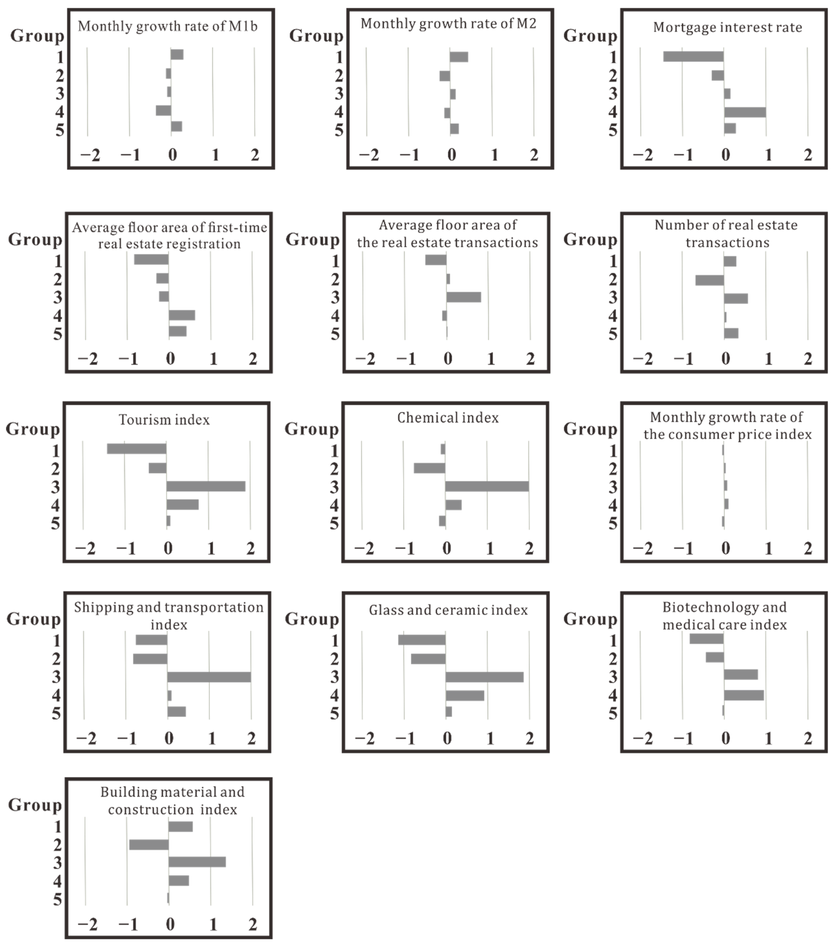
A total of 13 indexes was closely related to money supply: (1) monthly growth rate of M1b, (2) monthly growth rate of M2, (3) mortgage interest rate, (4) average floor area of first-time real estate registrations, (5) average floor area in real estate transactions, (6) number of real estate transactions, (7) tourism index, (8) chemical index, (9) monthly growth rate of the consumer price index, (10) shipping and transportation index, (11) glass and ceramic index, (12) biotechnology and health care index, and (13) building material and construction index.
After performing data clustering, we further analyzed money supply. The money supply indicators are presented in Table 1. In the ANOVA, the R2 value was 0.99, where this high value indicated the high explanatory power of all the indicators for money supply. The monthly growth rates of M1b and M2 reflected the state of Taiwan’s money supply, and the mortgage interest rates stimulated consumers’ willingness to buy real estate. These indicators represented the financial resources that affected the purchase of real estate. Money supply also indirectly affected the average floor area of first-time real estate registrations, average floor area of the property, and number of property transactions. Our findings indicated that tourism, chemical, shipping and transportation, glass and ceramic, biotechnology and health care, and building materials and structural indexes may affect the stock market.

Table 1.
Descriptive statistics of indexes related to money supply from January 2009 to December 2020.
Figure 1 illustrates the clustering results based on 13 indexes related to trends in money supply using DBM-PSO. The clustering of five groups provided the optimal sum of intracluster distances within all clusters compared with other numbers of clustering groups. Each bar indicates the average of the clustered samples in an index related to money supply. The positive and negative numbers are the high and low numbers in an index. The results revealed that the clustering results were similar in terms of the mortgage interest rate, average floor area in first-time real estate registration, tourism index, chemical index, shipping and transportation index, glass and ceramic index, and biotechnology and medical care index. The average floor area in real estate transactions was correlated with these six stock indexes, as illustrated in Figure 1. The results demonstrated that the average floor area of the first real estate registration and average floor area of properties were highly correlated with mortgage interest rates. With a monthly growth rate in M2, the real estate transaction volume increased. Therefore, an increase in mortgage interest rates increased the average floor area of transaction properties, and a decline reduced the average floor area.
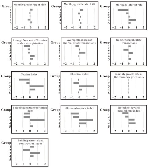
Figure 1.
Average value of characters in monthly clustering results related to money supply.
Our results demonstrated that money supply strongly influenced real estate trends. In their study, Goodhart and Hofmann noted that an increase in money supply [36] led to a positive response in house prices by changing the balance between cash and other liquid assets, and White noted that money supply permanently affected UK house prices [37]. In this study, we observed that money supply profoundly affected the floor area of first-time real estate registrations. When house prices in Taiwan rise, buying a house is challenging for young people. Consequently, the government lowers mortgage rates to accelerate corporate investment in the real estate market; a lower loan interest rate facilitates the buying of a first house. Simultaneously, money supply in the real estate market also increases. To keep up with market demand, developers reduce the floor area of apartment blocks to increase people’s willingness to buy and the number of real estate transactions. When the money supply increases, the real estate transaction volume and house prices also increase; simultaneously, the floor area of apartment blocks decreases. Therefore, as an intermediate objective of monetary policy, money supply could influence investors’ decisions related to the real estate market [38]. We identified specific stocks, related to the travel, chemical, shipping and transportation, glass and ceramic, biotechnology and health care, building material, and construction industries, in which money supply affected the stock market.
4.2. Population
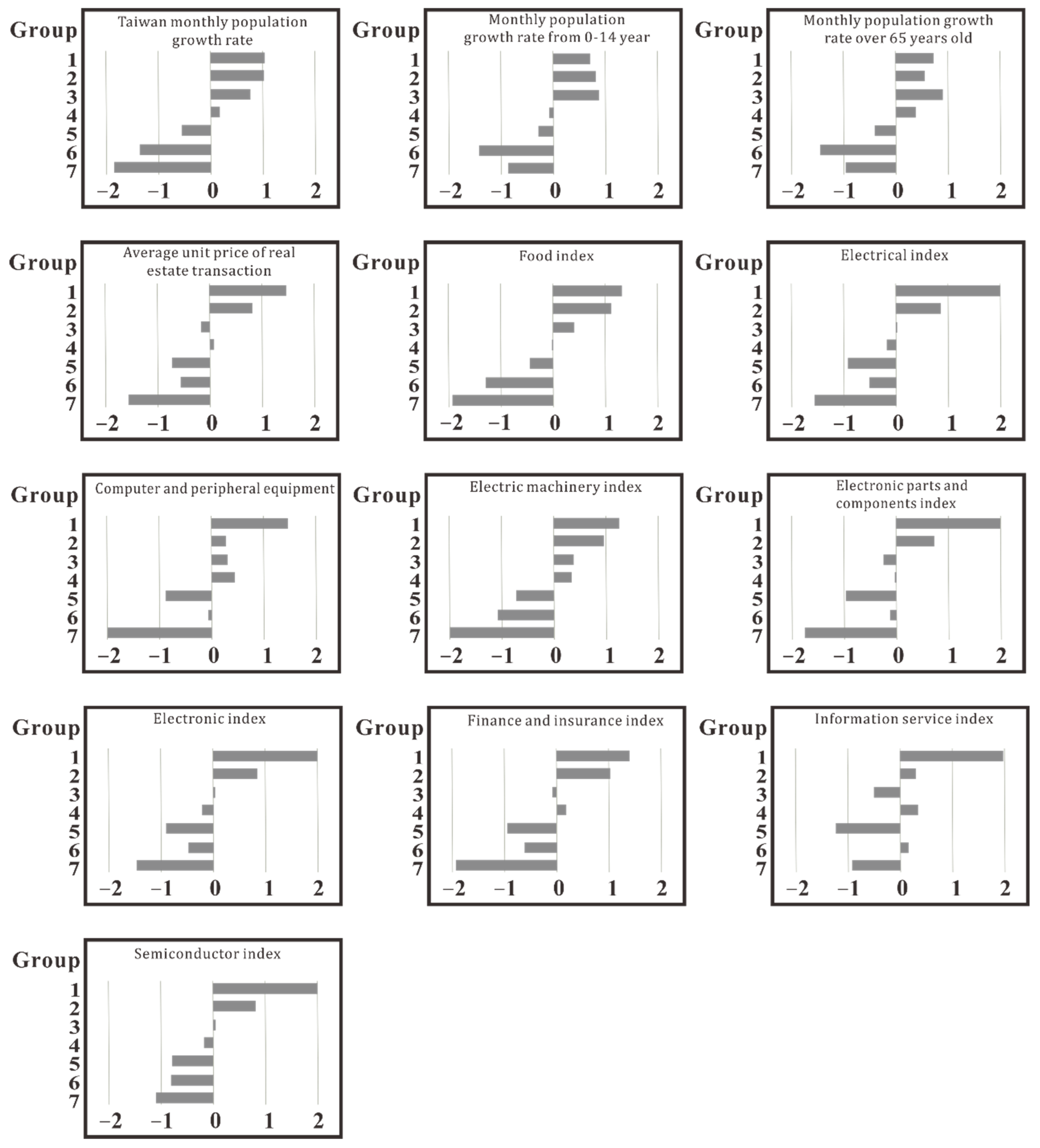
The following 13 indexes were closely related to population: (1) Taiwan’s monthly population growth rate, (2) the monthly population growth rate of people aged 0–14 years, (3) monthly population growth rate of people aged > 65 years, (4) average unit price of real estate transactions, (5) food index, (6) electrical index, (7) computer and peripheral equipment index, (8) electric machinery index, (9) electronic parts and components index, (10) electronic index, (11) finance and insurance index, (12) information service index, and (13) semiconductor index.
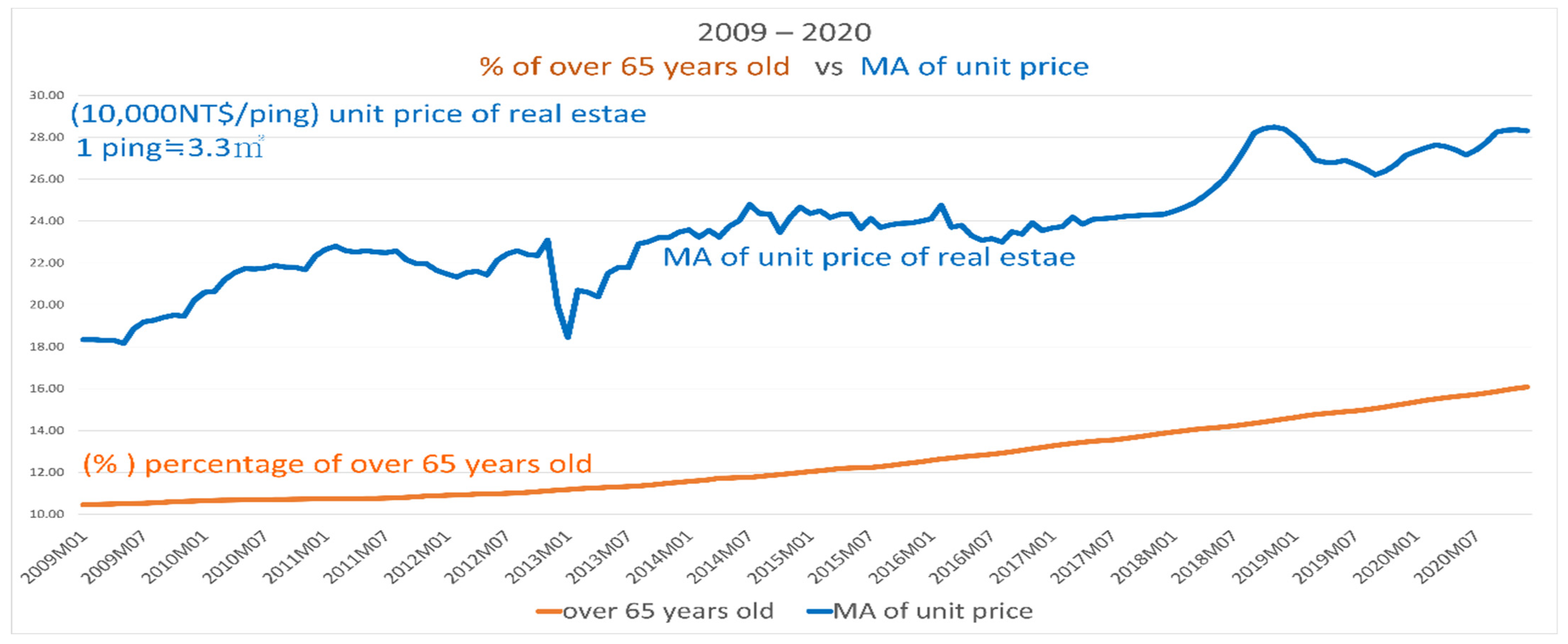
These indicators were related to the population index and affected the average unit price of property transactions and the stock market. The post clustering descriptive statistics of the population indicators are presented in Table 2. The R2 value was 0.99, which was satisfactory. Taiwan’s population increased for decades before decreasing from 23.6 million in 2019. Figure 2 presents the clustering results based on 13 indexes related to population using DBM-PSO. The results revealed 13 indexes with similar clustering results. From 2009 to 2020, the population grew in line with the average unit price of real estate transactions (Figure 2). Taiwan became an aging society in 1993 and is expected to be a super-aged society by 2025. Although the population growth rate has declined since 2020, the average unit price of real estate transactions has increased. This trend demonstrates that the monthly growth rate of the population >65 years has led to a continual increase in the average unit price of construction transactions. The population is rapidly aging, as depicted in Figure 2. By 2020, the older adult population increased rapidly, but the unit price of real estate increased more slowly.
Table 2.
Descriptive statistics of indexes related to population group from January 2009 to December 2020.

Figure 2.
Monthly growth rate of people aged > 65 years with MA of unit price from 2009 to 2020.
According to a report by the National Development Council of Taiwan, the super-aged (aged > 85 years) population accounted for 10.3% of the older adult population in 2020, and might increase to 27.4% by 2070. The percentage of the population that is young and middle-aged, the age groups generally interested in purchasing real estate, continues to decrease. However, Taiwan’s housing prices have not fallen in the past 10 years. In Taiwan, older adults (aged ≥ 65 years) are relatively financially stable because they have accumulated wealth and can afford expensive houses. Additionally, older people may focus more on insurance and asset inheritance, which may have caused the financial insurance index to rise with the monthly growth rate of the population > 65. The growth of Taiwan’s electronics and semiconductor stock markets may also be closely related to the growth of the older population, as illustrated in Figure 3.
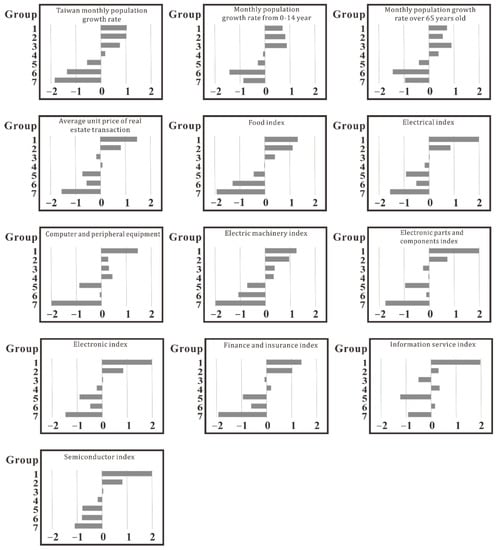
Figure 3.
Average value of character in monthly clustering results related to population group.
Our results revealed that population size affected real estate and reaffirmed the conclusions of other studies. Otto demonstrated that population growth had a significant positive effect [39], Takáts noted that demographics significantly affected real house prices, and Tsai et al. identified population density to be a key factor affecting house price spread [40]. Furthermore, the present study revealed that the average unit price of real estate transactions influenced by population was higher than the number of real estate transactions and the average floor area of real estate transactions. Bensdorp demonstrated that the effect of demographics on real estate was significant [41]. Older people accumulate wealth during their lifetime and spend more on housing. Although they do not require a large house, they require a comfortable house. Therefore, the average unit price of real estate transactions influenced by population was higher than that of other prices. This study divided the population into three groups based on age. Our results demonstrated that different population age groups had different effects on real estate. The monthly growth rate of the >65 population was more likely to affect the average unit price of real estate transactions than that of other age groups. Wang and Kinugasa demonstrated that a 1% increase in the old-age dependency ratio led to a 5.51% increase in house prices [42], and Gevorgyan revealed that when the population increased by 1%, house prices increased by 1.4% [43]. The older adult population can influence real estate positively; for example, it affects stock markets, including those linked to the food, power, electrical, electronic components, electronics, financial and insurance, information services, and semiconductor industries.
4.3. Rent
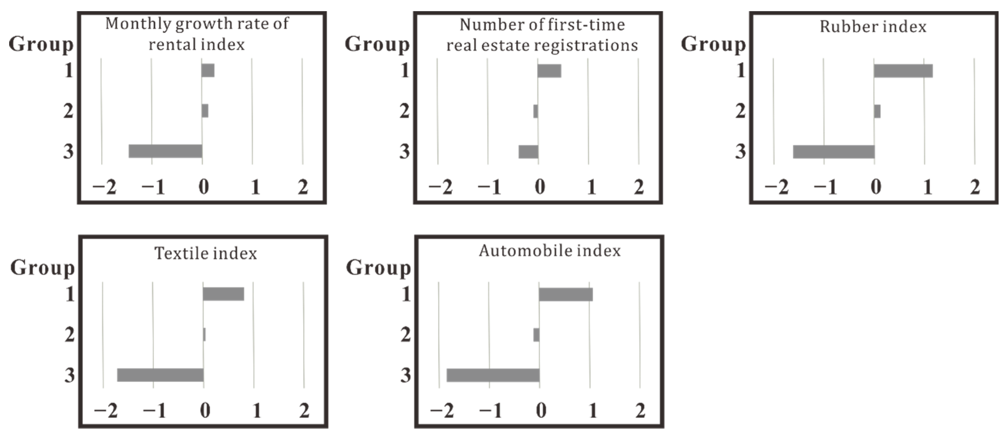
Five indexes were closely related to rent: (1) the monthly growth rate of the rental index, (2) number of first-time real estate registrations, (3) rubber index, (4) textile index, and (5) automobile index.
All rent indicators were closely related to rent trends, and the average values associated with rent are illustrated in Table 3. The R2 value was 0.72, which indicates a suitable correlation. Figure 4 presents the clustering results based on five indexes related to rent using DBM-PSO. The results indicated that these indexes had similar clustering results. In traditional Taiwanese society, older adult people often purchase real estate as an asset to pass on to the next generation. However, this practice is not popular among the younger generation. In particular, the marriage rate among young people continues to decline, and the divorce rate has risen, stimulating the housing rental market. The younger generation no longer regards buying a house as a goal; therefore, many young people rent to avoid being burdened with a lifetime mortgage. The monthly growth rate of the rent index represents the rise and fall of rental prices. When the monthly growth rate increases, construction companies may invest in building houses, and the number of first-time real estate registrations may increase. Because the younger generation tends not to have a mortgage, they have more capital to purchase cars, clothes, and furniture, as indicated by a rise in the rubber, textile, and automobile stock indexes. The monthly growth rate of the rent index increases with the number of first-time real estate registrations, possibly promoting consumer activity in the automobile, rubber, textiles, and stock markets.
Table 3.
Descriptive statistics of indexes related to the rental group from January 2009 to December 2020.
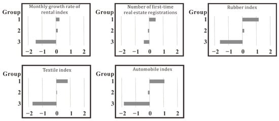
Figure 4.
Average value of character in the monthly clustering result is related to the rental group.
In economic theory, rents determine real estate prices, and prices also affect the rents offered. If we were to use traditional analytical methods, the volatility of rental growth could be significantly underestimated. Li et al. argued that the urban rental housing market is determined by regional-level factors such as employment opportunities, wage levels, and the “floating” population [44]. Hirota et al. noted that contracts with higher rents lead to price increases in housing markets [45]; a positive interaction exists between real estate prices and rents in the real economy. Zhai et al. noted that the rent-to-price ratio is a critical quota that reflects the health of the real estate market [46]. As rental demand increases, rents also rise, pushing up property prices; therefore, the amount of new real estate is bound to increase. When rents increase, construction companies can invest in new buildings, and more properties can then be registered for the first time. Furthermore, our results revealed that the monthly growth rate of the rental index was positively correlated with the number of first-time real estate registrations. This monthly growth rate could affect stocks in the rubber, textile, and automobile sectors. In Taiwan, young people do not want lifetime mortgages, and newlyweds prefer renting. More people are renting, house prices are rising, and investors are buying more homes. This trend has set a record for steady growth in Taiwanese real estate.
Money supply, population, and rent certainly affect the real estate trend. Many researchers have concluded previous research. Su et al. proved that money supply could control real estate prices to a certain extent [47]. Zhang et al. mentioned that population factors play a substantial and long-term role in the Chinese real estate market [48]. Baird et al. found that residential sales prices rose 0.95%, commercial sales rose 2.7%, and rental prices rose 0.55% [49]. In this study, we collected sociodemographic and socioeconomic information from open government sources and then standardized and clustered the data to determine that money supply, population, and rent were related to real estate trends. Our findings were further synthesized to draw the following three conclusions: (1) the influence of money supply trends on the construction area of real estate, (2) the effect of population trends on the unit price of real estate, and (3) the effect of rent on the trend of first-time registration of real estate. The three factors were summarized as follows.
4.4. Effect of Money Supply on the Floor Area of Property
The effect of money supply on real estate has been determined in previous studies. Xu found that China’s monetary policy actions are the critical driver behind China’s property price growth [50]. Oni et al. found that money supply in the economy, the source of funds for real estate development, is significantly affected by the indicator, so the allocation of funds to the real estate industry reduces the impact on the real estate industry [51]. Dissimilar to past studies, our findings demonstrated that money supply strongly influences real estate trends. Primarily, it had a profound effect on the average floor area of first-time real estate registrations. The rising average floor area of registered properties indicated that construction companies invest more in developing new buildings when they have sufficient funds, stimulating the real estate market. We suggest further research on the type of houses that may be constructed in the future, because large houses become popular when the money supply increases. We also determined that money supply affected specific stocks in the stock market, such as the travel, chemical, shipping and transportation, glass and ceramic, biotechnology and health care, building material, and construction industries.
4.5. Effect of Population on the Unit Price of Property
Wang et al. investigated how population aging and mobility affect housing prices at the city level. They found that the impact of policies plays a moderating role in the relationship between population structure and housing prices [52]. Our results also demonstrated that population also affected real estate. Tsai et al. indicated that population density was the main factor affecting the spread of housing prices [53]. The average unit price of real estate transactions affected by the population was higher than the number of real estate transactions and average floor area in real estate transactions. We divided the population into three categories according to age. The results indicated that the monthly growth rate of the >65 year-old population was more likely to affect the average unit price of real estate transactions than that of people in other age categories. The population also affected the stock market, including the food, electrical, motor, electronic component, finance and insurance, information service, and semiconductor industries.
4.6. Effect of Rent on First-Time Real Estate Registrations
The rent-to-price ratio is a crucial indicator of the property market’s health. Zhai et al. verified that house price and rent have an endogenous relationship [46]. Xu et al. found that the dynamics between house prices, rents, and structural age have implications for real estate valuations and house price index construction [54]. The traditional view of the real estate market is highly localized [55]. If we used the traditional analytical approach, the volatility in rent growth may be significantly underestimated. In the clustering results, the monthly growth rate of the rent index was positively correlated with the number of first-time real estate registrations. When rent increases, construction companies may invest additional funds, and more people register for the first time. Research has indicated that the monthly growth rate of the rent index also affects the stock markets for the rubber, textile, and automobile industries. In Taiwan, after 1980, a new trend emerged of young people not wanting a lifetime mortgage, and newlyweds preferred to rent a house. Because more people rented houses, housing prices rose, and investors purchased more houses. This trend created a record of steady growth in Taiwan’s real estate.
Many researchers studied sustainable urban governance networks. Mitchell T. et al. analyzed the results of an exploratory review on big data-driven urban geopolitics, connected sensor networks, and spatial cognitive computing in smart city software systems [56]. We can further study money supply, population, and rent in real estate trend analyses using urban sensing technology and geospatial big data analyses. Hudson et al. mentioned that machine learning-based analytics and big data applications are leveraged throughout smart, sustainable cities [57]. Therefore, citizen-centric data governance mechanisms and data-based value creation contribute to the sustainable social development of smart cities [58]. In the future, smart city technologies will include IoT devices and socio-technical interconnected systems that articulate organizational and institutional processes throughout urban governance [59].
One of the techniques helpful in segmenting economic and functional data is clustering, which has been widely used in various studies [60]. The K-means algorithm has been widely used in credit ratings [61] and real estate investment; however, it has a poor implementation in related studies concerning the clustering analysis [28,62]. Dissimilar to previous studies that adopted the K-means algorithm as the clustering technique, this study applied a group-based optimization method using improved particle swarm optimization (PSO) to increase the accuracy of the clustering. The advantage of group-based optimization methods is that efficient recurrent structures (or best overall patterns of clusters) can be obtained [63]. This segment-based approach has the advantage of studying the impact of individual segments on real estate by assessing feature similarities across sets. The advantage of our analytical framework based on the DBM-PSO clustering algorithm is that we formulated the soft-constrained clustering problem as a single optimization problem, rather than a typical exploration of the impact of a single feature on real estate, where the problem was solved as a hard-constrained problem and then the results were updated [64]. The disadvantage of this approach was that the behavioral effects of other real estate features were treated entirely as part of the model, i.e., the feature recognition ability for noise was poor. Furthermore, the advantage of the DBM map over other chaos maps was that it provided three high-frequency regions that varied over time, 0.0, 0.5, and 1.0. Distribution ratios of 0.0, 0.5, and 1.0 could effectively balance the particle search behavior in exploration and exploitation. Therefore, DBM-PSO had superior exploration and exploitation advantages in the search process and could outperform other clustering algorithms. Furthermore, DBM-PSO was only used to enhance the PSO update equation, so DBM-PSO did not increase the complexity of the PSO search process.
The proposed utilization of our analytical framework based on the DBM-PSO clustering algorithm could be summarized as follows: the DBM-PSO clustering algorithm defined K center locations for K clusters, where K is the total number of clusters. The parameter F is the total number of features in the dataset. The K × F dimension of a particle can be generated as a cluster solution, where the F interval in this dimension represents a center point. The Euclidean distance was used to evaluate the intra-cluster distance, and the short intra-cluster distance represents the better cluster solution. In DBM-PSO, gbest indicates the optimal clustering solution in each iteration, and the final solution was obtained from gbest in the last iteration. The solution includes the Kth center point and then assigns each dataset sample into a cluster based on the shortest distance between the sample vector and the cluster. Therefore, specific segmented tags could be obtained to understand the characteristics of each group for real estate marketing and analysis of marketing strategies.
5. Conclusions
In this study, we proposed an analytical framework to determine which features affect real estate based on the DBM-PSO clustering algorithm and identified three factors: money supply, population, and rent. This study provided an approach to real estate data clustering through which raw data can be analyzed and applied to real estate trend forecasting. We reported three findings that affected the real estate transaction market in Taiwan: (1) money supply affected the real estate floor area, (2) population trends affected the unit price of real estate, and (3) rent trends affected first-time real estate registration. These results helped the government to manage the relationship between the rental and real estate markets.
Based on research, we found that money supply, population and rent directly affected real estate. The money supply indirectly affected the average floor area of real estate holdings. The population correlated with the average unit price of real estate, and rental properties were associated with the number of first-time real estate registrations. This research provided a fundamental method of real estate data clustering through which original data can be analyzed and encoded data clustered, which can be applied to real estate trend predictions. The government could control the above three factors by formulating relevant laws and regulations in advance. Most real estate trend factors were related to government legislation. Therefore, when the government formulates relevant laws and regulations, it should take into account people’s housing justice. A limitation of this study was data collection, as we focused on Taiwan for the regional study. A future research perspective is to conduct a global analysis of Asia.
Supplementary Materials
The following supporting information can be downloaded at: https://www.mdpi.com/article/10.3390/math10071155/s1; Table S1: Descriptive statistics of 98 index.
Author Contributions
C.-H.Y.: project administration. B.L.: conceptualization, methodology, writing—review and editing, project administration. Y.-D.L.: conceptualization, project administration. All authors have read and agreed to the published version of the manuscript.
Funding
The funding sources were the Ministry of Science and Technology, Taiwan (under grant no. 108-2221-E-992-031-MY3 and 110-2222-E-346-002-).
Institutional Review Board Statement
Not applicable.
Informed Consent Statement
Not applicable.
Data Availability Statement
Not applicable.
Conflicts of Interest
The authors declare no conflict of interest.
References
- Ratcliffe, J.; Stubbs, M.; Keeping, M. Urban Planning and Real Estate Development; Routledge: New York, NY, USA, 2021. [Google Scholar]
- Mikulić, J.; Vizek, M.; Stojčić, N.; Payne, J.E.; Časni, A.Č.; Barbić, T. The effect of tourism activity on housing affordability. Ann. Tour. Res. 2021, 90, 103264. [Google Scholar] [CrossRef]
- Hu, C.-P.; Hu, T.-S.; Fan, P.; Lin, H.-P. The urban blight costs in taiwan. Sustainability 2021, 13, 113. [Google Scholar] [CrossRef]
- Baldominos, A.; Blanco, I.; Moreno, A.J.; Iturrarte, R.; Bernárdez, Ó.; Afonso, C. Identifying real estate opportunities using machine learning. Appl. Sci. 2018, 8, 2321. [Google Scholar] [CrossRef] [Green Version]
- Liu, C.; Xiong, W. China’s real estate market. In The Handbook of China’s Financial System; Walter de Gruyter, Inc.: Berlin, Germany, 2020; pp. 183–207. [Google Scholar]
- Chen, Y.-L. “Housing prices never fall”: The development of housing finance in taiwan. In Housing Policy Debate; Informa PLC: London, UK, 2020; Volume 30, pp. 623–639. [Google Scholar]
- Chang, C.-O.; Chen, S.-M. Dilemma of housing demand in taiwan. Int. Real Estate Rev. 2018, 21, 397–418. [Google Scholar] [CrossRef]
- Zinchenko, O.; Finahina, O.; Pankova, L.; Buriak, I.; Kovalenko, Y. Investing in the development of information infrastructure for technology transfer under the conditions of a regional market. East.-Eur. J. Enterp. Technol. 2021, 3, 111. [Google Scholar]
- Salvati, L.; Ciommi, M.T.; Serra, P.; Chelli, F.M. Exploring the spatial structure of housing prices under economic expansion and stagnation: The role of socio-demographic factors in metropolitan rome, italy. Land Use Policy 2019, 81, 143–152. [Google Scholar] [CrossRef]
- Lizares, R.M.; Bautista, C.C. Corporate financial distress: The case of publicly listed firms in an emerging market economy. J. Int. Financ. Manag. Account. 2021, 32, 5–20. [Google Scholar] [CrossRef]
- Morano, P.; Tajani, F.; Di Liddo, F.; Darò, M. Economic evaluation of the indoor environmental quality of buildings: The noise pollution effects on housing prices in the city of bari (italy). Buildings 2021, 11, 213. [Google Scholar] [CrossRef]
- Renigier-Biłozor, M.; Źróbek, S.; Walacik, M.; Borst, R.; Grover, R.; d’Amato, M. International acceptance of automated modern tools use must-have for sustainable real estate market development. Land Use Policy 2022, 113, 105876. [Google Scholar] [CrossRef]
- Wang, X.; Wen, J.; Zhang, Y.; Wang, Y. Real estate price forecasting based on svm optimized by pso. Optik 2014, 125, 1439–1443. [Google Scholar] [CrossRef]
- Mooya, M.M. Real Estate Valuation Theory: A Critical Appraisal, 1st ed.; Springer: Berlin/Heidelberg, Germany, 2016; 185p. [Google Scholar]
- Yang, L.; Chu, X.; Gou, Z.; Yang, H.; Lu, Y.; Huang, W. Accessibility and proximity effects of bus rapid transit on housing prices: Heterogeneity across price quantiles and space. J. Transp. Geogr. 2020, 88, 102850. [Google Scholar] [CrossRef]
- Öztürk, A.; Kapusuz, Y.E.; Tanrıvermiş, H. The dynamics of housing affordability and housing demand analysis in ankara. Int. J. Hous. Mark. Anal. 2018, 11, 828–851. [Google Scholar] [CrossRef]
- Alkay, E.; Watkins, C.; Keskin, B. Explaining spatial variation in housing construction activity in turkey. Int. J. Strateg. Prop. Manag. 2018, 22, 119–130. [Google Scholar] [CrossRef] [Green Version]
- Coskun, Y.; Seven, U.; Ertugrul, H.M.; Alp, A. Housing price dynamics and bubble risk: The case of turkey. Hous. Stud. 2020, 35, 50–86. [Google Scholar] [CrossRef]
- Kirikkaleli, D.; Athari, S.A.; Ertugrul, H.M. The real estate industry in turkey: A time series analysis. Serv. Ind. J. 2018, 41, 427–439. [Google Scholar] [CrossRef]
- Stephany, F.; Stoehr, N.; Darius, P.; Neuhäuser, L.; Teutloff, O.; Braesemann, F. The corisk-index: A data-mining approach to identify industry-specific risk assessments related to covid-19 in real-time. arXiv 2020, arXiv:2003.12432. [Google Scholar] [CrossRef]
- Yang, Y.; Altschuler, B.; Liang, Z.; Li, X.R. Monitoring the global covid-19 impact on tourism: The covid19tourism index. Ann. Tour. Res. 2021, 90, 103120. [Google Scholar] [CrossRef]
- Sun, J.; Yang, X.; Zhao, X. Understanding commercial real estate indices. J. Real Estate Portf. Manag. 2020, 18, 289–303. [Google Scholar] [CrossRef]
- Usman, H.; Lizam, M.; Adekunle, M.U. Property price modelling, market segmentation and submarket classifications: A review. Real Estate Manag. Valuat. 2020, 28, 24–35. [Google Scholar] [CrossRef]
- Mittal, M.; Goyal, L.M.; Hemanth, D.J.; Sethi, J.K. Clustering approaches for high-dimensional databases: A review. Wiley Interdiscip. Rev. Data Min. Knowl. Discov. 2019, 9, e1300. [Google Scholar] [CrossRef]
- Yang, C.-H.; Chuang, L.-Y.; Lin, Y.-D. Epistasis analysis using an improved fuzzy c-means-based entropy approach. IEEE Trans. Fuzzy Syst. 2019, 28, 718–730. [Google Scholar] [CrossRef]
- Kan-Kilinc, B.; Tug, I. The Examination of Real Estate Prices in Istanbul by Using Hybrid Hierarchical K-Means Clustering (Betul 2019). In Proceedings of the y-BIS 2019 Conference Book: Recent Advances in Data Science and Business Analytics, Istanbul, Turkey, 25–28 September 2019. [Google Scholar]
- Liao, S.-H.; Chou, S.-Y. Data mining investigation of co-movements on the taiwan and china stock markets for future investment portfolio. Expert Syst. Appl. 2013, 40, 1542–1554. [Google Scholar] [CrossRef]
- Chuang, L.-Y.; Lin, Y.-D.; Yang, C.-H. Data clustering using chaotic particle swarm optimization. IAENG Int. J. Comput. Sci. 2012, 39, IJCS_39_32_08. [Google Scholar]
- Kennedy, J.; Eberhart, R. Particle swarm optimization. In Proceedings of the ICNN’95-International Conference on Neural Networks, Perth, WA, Australia, 27 November–1 December 1995; pp. 1942–1948. [Google Scholar]
- Shi, Y.; Eberhart, R.C. Empirical study of particle swarm optimization. In Proceedings of the 1999 Congress on Evolutionary Computation-CEC99 (Cat. No. 99TH8406), Washington, DC, USA, 6–9 July 1999; IEEE: Washington, DC, USA, 1999; Volume 3, pp. 1945–1950. [Google Scholar]
- Yang, C.-H.; Tsai, S.-W.; Chuang, L.-Y.; Yang, C.-H. An improved particle swarm optimization with double-bottom chaotic maps for numerical optimization. Appl. Math. Comput. 2012, 219, 260–279. [Google Scholar] [CrossRef]
- Yang, C.-H.; Lin, Y.-D.; Chuang, L.-Y.; Chang, H.-W. Double-bottom chaotic map particle swarm optimization based on chi-square test to determine gene-gene interactions. BioMed Res. Int. 2014, 2014, 172049. [Google Scholar] [CrossRef]
- McCarthy, R.V.; McCarthy, M.M.; Ceccucci, W.; Halawi, L. What do descriptive statistics tell us. In Applying Predictive Analytics; Springer: Cham, Switzerland, 2019; pp. 57–87. [Google Scholar]
- Gelman, A. Analysis of variance—why it is more important than ever. Ann. Stat. 2005, 33, 1–53. [Google Scholar] [CrossRef] [Green Version]
- Kumari, K.; Yadav, S. Linear regression analysis study. J. Pract. Cardiovasc. Sci. 2018, 4, 33. [Google Scholar] [CrossRef]
- Goodhart, C.; Hofmann, B. House prices, money, credit, and the macroeconomy. Oxf. Rev. Econ. Policy 2008, 24, 180–205. [Google Scholar] [CrossRef] [Green Version]
- White, M. Cyclical and structural change in the uk housing market. J. Eur. Real Estate Res. 2015, 8, 85–103. [Google Scholar] [CrossRef] [Green Version]
- Bouchouicha, R.; Ftiti, Z. Real estate markets and the macroeconomy: A dynamic coherence framework. Econ. Model. 2012, 29, 1820–1829. [Google Scholar] [CrossRef]
- Otto, G. The growth of house prices in australian capital cities: What do economic fundamentals explain? Aust. Econ. Rev. 2007, 40, 225–238. [Google Scholar] [CrossRef]
- Takáts, E. Aging and house prices. J. Hous. Econ. 2012, 21, 131–141. [Google Scholar] [CrossRef]
- Bensdorp, V. Influence of Population Demographics on Real Estate Prices in Zuid-Holland. Master’s Thesis, Utrechr University, Utrecht, The Netherlands, 2021. [Google Scholar]
- Wang, Y.; Kinugasa, T. The relationship between demographic change and house price: Chinese evidence. Int. J. Econ. Policy Stud. 2021, 16, 43–65. [Google Scholar] [CrossRef]
- Gevorgyan, K. Do demographic changes affect house prices? J. Demogr. Econ. 2019, 85, 305–320. [Google Scholar] [CrossRef] [Green Version]
- Li, H.; Wei, Y.D.; Wu, Y. Analyzing the private rental housing market in shanghai with open data. Land Use Policy 2019, 85, 271–284. [Google Scholar] [CrossRef]
- Hirota, S.; Suzuki-Löffelholz, K.; Udagawa, D. Does owners’ purchase price affect rent offered? Experimental evidence. J. Behav. Exp. Financ. 2020, 25, 100260. [Google Scholar] [CrossRef]
- Zhai, D.; Shang, Y.; Wen, H.; Ye, J. Housing price, housing rent, and rent-price ratio: Evidence from 30 cities in china. J. Urban Plan. Dev. 2018, 144, 04017026. [Google Scholar] [CrossRef]
- Su, C.-W.; Wang, X.-Q.; Tao, R.; Chang, H.-L. Does money supply drive housing prices in china? Int. Rev. Econ. Financ. 2019, 60, 85–94. [Google Scholar] [CrossRef]
- Zhang, H.; Lu, T.; Sun, Y. Research on the development of real estate market based on population change in China. Proc. IOP Conf. Ser. Earth Environ. Sci. 2019, 267, 062031. [Google Scholar] [CrossRef]
- Baird, M.D.; Schwartz, H.; Hunter, G.P.; Gary-Webb, T.L.; Ghosh-Dastidar, B.; Dubowitz, T.; Troxel, W.M. Does large-scale neighborhood reinvestment work? Effects of public–private real estate investment on local sales prices, rental prices, and crime rates. Hous. Policy Debate 2020, 30, 164–190. [Google Scholar] [CrossRef]
- Xu, X.E.; Chen, T. The effect of monetary policy on real estate price growth in china. Pac.-Basin Financ. J. 2012, 20, 62–77. [Google Scholar] [CrossRef]
- Oni, A.; Emoh, F.; Ijasan, K. The impact of money market indicators on real estate finance in nigeria. Sri Lankan J. Real Estate 2012, 6, 16–37. [Google Scholar]
- Wang, X.; Hui, E.C.-M.; Sun, J. Population aging, mobility, and real estate price: Evidence from cities in china. Sustainability 2018, 10, 3140. [Google Scholar] [CrossRef] [Green Version]
- Tsai, I.C. Housing price convergence, transportation infrastructure and dynamic regional population relocation. Habitat Int. 2018, 79, 61–73. [Google Scholar] [CrossRef]
- Xu, Y.; Zhang, Q.; Zheng, S.; Zhu, G. House age, price and rent: Implications from land-structure decomposition. J. Real Estate Financ. Econ. 2018, 56, 303–324. [Google Scholar] [CrossRef] [Green Version]
- An, X.; Deng, Y.; Fisher, J.D.; Hu, M.R. Commercial real estate rental index: A dynamic panel data model estimation. Real Estate Econ. 2016, 44, 378–410. [Google Scholar] [CrossRef]
- Mitchell, T.; Krulicky, T. Big data-driven urban geopolitics, interconnected sensor networks, and spatial cognition algorithms in smart city software systems. Geopolit. Hist. Int. Relat. 2021, 13, 9–22. [Google Scholar]
- Hudson, L.; Sedlackova, A.N. Urban sensing technologies and geospatial big data analytics in internet of things-enabled smart cities. Geopolit. Hist. Int. Relat. 2021, 13, 37–50. [Google Scholar]
- Evans, V.; Horak, J. Sustainable urban governance networks, data-driven internet of things systems, and wireless sensor-based applications in smart city logistics. Geopolit. Hist. Int. Relat. 2021, 13, 65–78. [Google Scholar]
- König, P.D. Citizen-centered data governance in the smart city: From ethics to accountability. Sustain. Cities Soc. 2021, 75, 103308. [Google Scholar] [CrossRef]
- Feng, Z.; Zhang, J. Nonparametric k-means algorithm with applications in economic and functional data. Commun. Stat.-Theory Methods 2022, 51, 537–551. [Google Scholar] [CrossRef]
- Dang, C.; Chen, X.; Yu, S.; Chen, R.; Yang, Y. Credit ratings of chinese households using factor scores and k-means clustering method. Int. Rev. Econ. Financ. 2022, 78, 309–320. [Google Scholar] [CrossRef]
- Chuang, L.-Y.; Lin, Y.-D.; Yang, C.-H. An improved particle swarm optimization for data clustering. In Proceedings of the International MultiConference of Engineers & Computer Scientist 2012, IMECS, Hong Kong, China, 14–16 March 2012; pp. 440–445. [Google Scholar]
- Cao, L.; Wang, Y.; Zhang, B.; Jin, Q.; Vasilakos, A.V. Gchar: An efficient group-based context—aware human activity recognition on smartphone. J. Parallel Distrib. Comput. 2018, 118, 67–80. [Google Scholar] [CrossRef]
- Larabi Marie-Sainte, S. A survey of particle swarm optimization techniques for solving university examination timetabling problem. Artif. Intell. Rev. 2015, 44, 537–546. [Google Scholar] [CrossRef]
Publisher’s Note: MDPI stays neutral with regard to jurisdictional claims in published maps and institutional affiliations. |
© 2022 by the authors. Licensee MDPI, Basel, Switzerland. This article is an open access article distributed under the terms and conditions of the Creative Commons Attribution (CC BY) license (https://creativecommons.org/licenses/by/4.0/).