Abstract
In this work, we study the optimal investment and premium control problem with the short-selling constraint under the mean-variance criterion. The claim process is assumed to follow the non-homogeneous compound Poisson process. The insurer invests the surplus in one risk-free asset and one risky asset described by the Heston model. Under these, we consider an optimization objective that maximizes the return (the expectation of terminal wealth) and minimizes the risk (the variance of terminal wealth). By constructing the extended Hamilton–Jacobi–Bellman (HJB) system with the dynamic programming method, the time-consistent strategies and the corresponding value function are obtained. Furthermore, we provide numerical examples to illustrate the effects of the model parameters on the optimal policies.
Keywords:
investment; premium control; short-selling constraint; mean-variance criterion; the extended HJB system MSC:
91G80; 93E20
1. Introduction
In recent years, optimal investment problems with various objectives in managing insurance risk management have received much attention, and many types of research have been conducted. One of the fundamental objectives that the insurer pursues is the minimization of the ruin probability, i.e., the probability of the event that the surplus becomes non-positive, which was first studied by Browne (1995) [1] under the assumptions that the surplus follows the diffusion approximation and the financial market adheres to the classic Black–Scholes model, consisting of one risk-free asset (bond) and one risky asset (stock). Hipp and Plum (2000) [2] studied the same investment problem for the insurer, using the classical Cramér-Lundburg (C-L) risk model. Some associated problems have been solved via the techniques of stochastic control; see Schmidli (2002) [3], Liu and Yang (2004) [4], and Promislow and Young (2005) [5]. Some scholars pay close attention to the expected utility maximization of the terminal wealth of insurers. Bi and Chen (2019) [6] investigated the optimal investment–reinsurance strategy in a risk model with two dependent classes of insurance business under the criterion of maximizing the expected exponential utility with the expected value premium principle and the variance premium principle. Zhang and Zhao (2020) [7] studied the optimal investment–reinsurance problem concerning thinning dependent risks to maximize the expected exponential utility of terminal wealth. In addition, some scholars focus on other optimization objectives, for instance, the mean-variance criterion. We refer readers to Li et al. (2017) [8], Xiao et al. (2019) [9], and Yuan et al. (2021) [10].
In modern financial theory, the mean-variance portfolio problem put forward by Markowitz (1952) [11] is considered to be a milestone. As a widely accepted optimization objective that maximizes the return and minimizes the risk, the conventional dynamic programming method cannot be applied directly, and the mean-variance problem is categorized as the time-inconsistent problem. Strotz (1955) [12] assumed that the insurer pre-commits to the target determined at the initial time and does not update at the subsequent dates, and pointed out precommitment strategies to deal with time inconsistency. Zhou and Li (2000) [13], and Li and Ng (2000) [14] turned Markowitz’s portfolio model into the linear–quadratic stochastic control problem, deriving the analytical optimal investment strategies and the efficient frontier. Breakthrough work on obtaining time-consistent strategies under the mean-variance criterion was carried out by Björk and Murgoci (2010) [15]. They examined a general time-inconsistent objective function, elaborated the problem as a non-cooperative game, and sought the time-consistent subgame perfect Nash equilibrium strategies. An extension of the standard dynamic programming equation called the extended Hamilton–Jacobi–Bellman system was constructed. Scholars applied this basic framework to investigate the optimal investment–reinsurance problem under the mean-variance criterion. Zeng and Li (2011) [16] adopted the Black–Scholes model and studied the optimal time-consistent investment–reinsurance strategies. Li and Li (2013) [17] acquired the optimal investment and proportion reinsurance strategies with state-dependent risk aversion under the mean-variance criterion. For more studies on this topic, interested readers are referred to Bai et al. (2020) [18] and Wang et al. (2021) [19], in addition to the references.
In the extensively studied C-L risk model, the claim process is a time homogeneous compound Poisson process, and the claim arrival rate is assumed to be constant. Zhou et al.(2017) [20] investigated the non-homogeneous compound Poisson model, and constructed a monotone function to depict the relationship between the claim arrival rate and the safety loading. They derived the optimal investment and premium control strategies to maximize the exponential utility of the terminal wealth and minimize the ruin probability. Jiang et al. (2020) [21] considered the optimal investment, premium control and reinsurance problem, where the surplus process follows the diffusion approximation for the non-homogeneous Poisson process with a time-varying intensity. Liu et al. (2020) [22] took model ambiguity into consideration and analyzed the optimal investment and premium control policies for the ambiguity aversion insurer (AAI).
In the majority of former studies, the risky asset’s price volatility was assumed to be constant or deterministic. However, empirical financial works, such as those of Beckers (1980) [23], or Hobson and Rogers (1998) [24], tend to support that volatility is stochastic. Taylor (1982) [25] introduced the stochastic volatility (SV) model, which accurately reflects the significant features of the asset price, such as the fat-tailedness of the return distribution, the volatility smiling, and the volatility clustering. To date, a variety of volatility models have been proposed, for example, the constant elasticity of variance (CEV) model proposed by Cox and Ross (1976) [26], the mean-reverting model developed by Hull and White (1987) [27], and the Heston model established by Heston (1993) [28]. Li et al. (2012) [29] adopted the Heston model to discuss the optimal investment and proportional reinsurance strategies under the mean-variance criterion. Lin and Qian (2016) [30] explored the optimal investment and proportional reinsurance strategies for an insurer under the CEV model to maximize the expectation of the terminal wealth while minimizing the variance. Zhu et al. (2019) [31] proposed the equilibrium investment and reinsurance strategies for two competitive insurers with relative performance concerns under the Heston model.
In the financial market, the short-selling constraint is one of the main factors that make models more realistic (Short-selling can be achieved by borrowing assets (securities or commodities) and selling them. The investor will later purchase the same number of securities to return them to the lender. If the price has fallen in the meantime, the investor will have made a profit equal to the difference. Conversely, if the price has risen, then the investor will bear a loss.). Worldwide, economic regulators seem inclined to restrict short-selling to decrease potential downward price cascades, and countries such as China have imposed restrictions on short-selling (In China, short-selling was allowed for large blue-chip stocks with good earnings performance and little price volatility on 31 March 2010. However, in 2015, short-selling was effectively banned due to legislative restrictions on borrowing stocks following the same year’s stock market crash.). Moreover, during the COVID-19 pandemic, short-selling was severely restricted or temporarily banned, with the European market tightening the rules on short-selling to stem the historic losses arising from the coronavirus pandemic. It is of great significance to research the associated optimal control problems without short-selling opportunities. Luo et al. (2008) [32] utilized stochastic control theory to study the optimal investment–reinsurance problem that minimizes the ruin probability in the presence of short-selling and borrowing constraints. Bai and Guo (2008) [33] adopted the drifted Brownian motion risk model, and studied the optimal investment–reinsurance problem of maximizing the expected exponential utility and minimizing the probability of ruin with short-selling constraint. Liu and Zhang (2011) [34] assumed that the claim process follows the jump-diffusion process, and explored the optimal investment and excess-of-loss reinsurance problem with the short-selling constraint. Bi and Guo (2013) [35] exploited the linear–quadratic (LQ) stochastic control theory to investigate the optimal reinsurance–investment problem for an insurer with the short-selling constraint under the mean-variance criterion. Huang et al. (2016) [36] obtained the closed-form of optimal investment and proportional reinsurance policies with the constraints of net profit and short-selling.
This work explores the optimal asset allocation and premium control strategies for insurers under the mean-variance criterion. We impose the short-selling constraint, i.e., we suppose that the dollar amount invested in risky assets should be equal to or greater than zero. We assume that the financial market is composed of one risk-free asset and one risky asset, which is driven by the Heston model. Exploiting the dynamic programming principle, we establish the extended HJB equations and derive the optimal investment and premium control policies. Furthermore, detailed numerical analyses are provided to explore the impact of model parameters on the optimal decision. This work could be regarded as a supplement and extension of the existing theoretical studies about the optimal investment and premium control for insurers and emphasize the expansion and generalization of the model. To sum up, this paper consists of the following three innovations:
- (1)
- We investigate the optimal investment and premium control strategies with the short-selling constraint under the Heston model. The closed-form expression of the optimal time-consistent strategies and the verification theorem is provided.
- (2)
- We suppose that the claim process satisfies the non-homogeneous compound Poisson process, which has not been discussed in the existing literature under the mean-variance criterion.
- (3)
- We analyze the impact of a premium control mechanism on the optimal investment strategies through the comparison of the determined premium problem and the controlled premium problem.
The rest of our paper is given as follows: In Section 2, we introduce the models and assumptions of the financial market. Section 3 describes the optimal control problem with the mean-variance criterion. Section 4 derives the equilibrium investment and premium control strategies by solving the extended HJB system. Numerical illustrations are provided in Section 5 to analyze our results. Section 6 provides the conclusion, and the Appendix A and Appendix B are devoted to the proofs of some results in this paper.
2. Model and Assumptions
In this section, we consider a financial market with the following assumptions: the insurer can continuously trade in the financial market without paying taxes. Let be a risk-neutral probability space with filtration , where refers to the market information up to time t. is a finite constant that describes the time horizon. We suppose that all of the random variables and stochastic processes are well-defined on and that any decision made at time t is based on .
2.1. Surplus Process
Supposing that the surplus process of the insurer follows the C-L risk model, and the surplus process can be described as below:
where c represents the fixed cost rate, is the premium income at time t, and is a compound Poisson process, which stands for the cumulative claim amount up to time t. is a non-homogeneous Poisson process with intensity . The claim sizes are supposed to be independent and identically distributed (i.i.d.) positive random variables independent of . The finite first-order and second-order moments are denoted and , respectively. In addition, the premium rate is calculated according to the expected value principle; namely, , where represents the insurer’s time-varying safety loading, and it can be found that the insurer adjusts the premium rate by changing the safety loading. In practice, we observed that the increases in the safety loading lead to a decrease in the market share, and the claim arrival rate also decreases. As a result, a strictly decreasing function should be adopted to describe the relationship between the safety loading and the claim arrival rate. The function , where , is strictly decreasing, mapping the safety loading to the claim arrival rate. We have , where represents the inverse of . According to the above, we have
where and represent the expectation and variance, respectively. It is reasonable to impose:
- for the finite number of latents assured in the market.
- , which could be interpreted as the extreme premium leading to the shrink in the market share, and there would not be any claim during the time period.
- . This indicates that the insurer cannot make a profit by collecting a positive premium without any insurance.
After some simple manipulations, we have
We approximate (3) by the nonlinear diffusion process presented below, and details can be found in Zhou et al. (2017) [20].
where is a standard Brownian motion. Moreover, we denote and rewrite the surplus process as
where . Thus, is a differentiable function mapping from to and . Similar to Liu et al. (2020) [22], we assume that is strictly concave and . According to Rolle Theorem, there exists a satisfying , at which attains its maximum.
It can be seen that in . The drift term of (5) is decreasing, but the volatility term is increasing, which is irrational. Therefore, is in the case when the insurer is risk averse. According to Liu et al. (2020) [22], matches all the above assumptions.
2.2. Financial Market and the Wealth Process
We assume that the risk-free asset possesses a fixed continuous compound return rate , as follows:
To capture the effect of the volatility risk, we choose the Heston model to describe the price process of the risky asset:
where , k, and are positive constants. reflects the appreciation rate of the risky asset. k represents the rate at which reverts to long-term variance . expresses the volatility, which determines the variance of . and are both standard Brownian motions, having and . Furthermore, we assume that is independent of and , and we require to ensure that zero is not accessible or is almost surely non-negative.
The insurer can dynamically invest in the financial market during the time horizon . The trading strategy is a pair of stochastic processes, where represents the dollar amount invested in the risky asset at time t. A restriction considered in our work is the prohibition of shorting the risky asset; that is, must be satisfied, but we still allow borrowing from the money market (at the interest rate). is the premium control variable. Thus, the dollar amount invested in the risk-free asset at time t is , where is the wealth process associated with . Afterward, is the solution of the following stochastic differential Equation (SDE):
Definition 1.
For a fixed , the trading strategy is considered to be admissible, if
- (1)
- , is progressively measurable.
- (2)
- is progressively measurable and .
- (3)
- Equation (8) has a pathwise unique solution on .
Let denotes the set of all admissible strategies.
3. Problem Formulation in a Game Theoretic Framework
The insurer employs the mean-variance criterion in our problem, which is quite significant in modern financial theory. The insurer wishes to maximize the return by the conditional expectation () but minimize the risk by the conditional variance (). The variance term has the non-linear function of the expected value of terminal wealth, which results in time inconsistency. The optimality concept differs at different initial times and states, i.e., the change in state with time yields new optimal portfolio policies, and the insurer may question which optimal portfolio policies to adopt unless already decided. Before a widely accepted method was proposed to deal with time-inconsistent problems, scholars studied static pre-commitment optimization problems as the investors remain committed to the optimal portfolio strategies evaluated initially, determined the optimal portfolio strategies at time 0, and followed them blindly to the terminal time T. The optimization problem is
is the risk aversion coefficient, which stands for the degree of risk aversion. The “consistent planning” proposed by Strotz (1955) [12] means that individuals reject the strategies that they will not follow. Those rational decision-makers are “non-committed” to the optimal strategies evaluated initially, and continuously re-evaluate the optimality criterion at each new time.
- is once continuously differentiable on , and is twice continuously differentiable on .
- , and once all partial derivatives of satisfy the polynomial growth condition on .
For any , the dynamic problem is
where , are conditional expectation and conditional variance based on and , respectively. Moreover, we also have , , .
Björk and Murgoci (2010) [15] examined a general time-inconsistent objective function, elaborated the problem as a non-cooperative game, and sought the time-consistent perfect Nash equilibrium strategies. The definition of the Nash equilibrium strategy is as follows:
Definition 2.
For any fixed arbitrarily initial point , choose and . We consider an admissible strategy and define the below control:
If
we say that the is the equilibrium strategy, and the corresponding equilibrium value function is defined by
We suppose that at any state , the insurer aims to find the equilibrium strategies and the corresponding equilibrium value function of the optimization problem. Björk and Murgoci (2010) [15] constructed the extension of the standard dynamic programming equation, called the extended Hamilton–Jacobi–Bellman equations, and pointed out that the equilibrium strategies obtained by solving the equations are the optimal time-consistent strategies.
Before providing the verification theorem, we define a variational operator. For any ,
The extended HJB equations for problem (10) are defined as below:
where
with , , for short.
Theorem 1.
(Verification Theorem) For , suppose that there exist , and with the following properties:
- (1)
- , and solve the extended HJB system (13).
- (2)
- realizes the supremum in (13).
- (3)
- , and belong to the space .
Then
is the equilibrium strategy,is the corresponding equilibrium value function and, .
Proof.
Appendix A provides the proof for the Verification Theorem. □
4. Solution to the Optimization Problem
In the present section, we construct the solution to the extended HJB system by variable change technique and obtain the optimal investment and premium control policies through the stochastic control approach. Moreover, we provide special cases by selecting particular values for the model parameter.
Theorem 2.
For the optimization problem (10), we denote
Thus, the optimal time-consistent investment and premium control strategies are provided by the following cases:
- Case I . ; or with .
In this case, the optimal strategies are given by
and the value function is , where
with
Under this assumption, we find that the insurer carries out insurance business and actively invests in the prosperous financial market .
- Case II . with .
The optimal strategies are given by
and the value function is . In this case, the insurer conducts insurance business actively and hopes to obtain profits through short-selling the risky asset in the unsatisfactory financial market. However, due to short-selling restrictions, the insurer has to adopt a conservative investment strategy and invest the entirety of the wealth into the risk-free asset .
Proof.
See Appendix B. □
The existence and uniqueness of the second equation of (14) and (15) seem obvious based on the assumptions on , and the details can be found in Appendix B. The optimal investment and premium control strategies are dependent on the financial and insurance market parameters, and the optimal premium control is driven by . Moreover, we designate a specific form of to express our results analytically in Remark 3.
Remark 1.
In order to analyze the impact of the short-selling constraint on the optimal strategies, we derived the optimal time-consistent investment and premium control strategies without the short-selling constraint.
We find that the short-selling constraint shows no effect on the premium control strategy, but urges the insurer to adopt relatively conservative and prudent portfolio strategies. Short-selling is highly risky and may cause massive losses. The short-selling constraint keeps the optimal investment fraction from being negative. The optimal investment fraction in Case II of Theorem 2 indicates that the consideration of the short-selling constraint halts the overly aggressive portfolio strategy. As the measure of the market price of financial risk λ decreases, the insurer should invest wealth into the risk-free asset instead of short-selling the risky asset.
Remark 2.
(GBM model) We investigate the same optimization problem, for which the price process of the risky asset is driven by the geometric Brownian motion, i.e.,
where the appreciation rate (additional returns from taking risks) and the market volatility are all the positive constants. The optimal investment and premium control strategies are given by
and the value function is
Remark 3.
(Specific function) For the practical application of the current model, we refer to Liu et al. (2020) [22] and assume that . Thus, the optimal policies are given by
- Case I. If ; or with .
The value function is , where
- Case II . If with .the value function is
Remark 4.
(The determined premium problem) We hope to analyze the impact of the premium control mechanism on the optimal investment strategies, assuming that the insurer’s surplus process follows the classic C-L risk model. Thus, the surplus process can be described as
Considering that is a homogeneous Poisson process with intensity , the premium income is calculated according to the expected value principle, where is the safety loading of the insurer. Other parameters were introduced in Section 2, and we omit them here. Adopting the diffusion approximation technique (Grandelln(1991) [37]), we rewrite as
and the wealth process associated with the trading strategy π follows
Applying a similar method as in Theorem 2, we derived the optimal investment strategy for the determined premium problem. We omit the details.
- Case I . If , or with , the optimal investment strategy is given byand the value function is , where
- Case II . If with , we obtain the following expressionsand the value function is .
We will illustrate the impact of the premium control mechanism on the optimal value function in Section 5 by comparing the two value functions, and .
5. Analysis of the Results and Numerical Illustration
In order to visualize the impact of model parameters on the optimal investment and premium control strategies, we illustrate and in (16) with the specified function form , . It is worth noting that the price of the risky asset is driven by the Heston model. For applicability in practice, we referred to Zhao et al. (2013) [38] in choosing the financial market parameters. Throughout the numerical analysis, the parameters follow Table 1 unless otherwise specified. When , the uncertainties of the risky asset price and its volatility have the same direction of change, and when , the uncertainties of and change in the opposite direction. Eraker et al. (2003) [39] estimated that , and herein, we assume that .

Table 1.
The parameter values of the model in numerical illustration.
We provide some sensitivity analysis on the effect of the model parameters on the optimal investment and premium control strategies. According to the optimal investmet strategy in (16), we derive
We calculate that
- (a)
- , if one of the following conditions holds:
- (i)
- and ;
- (ii)
- and ;
- (iii)
- and ;
- (b)
- , if one of the following conditions holds:
- (iv)
- and ;
- (v)
- and ;
- (vi)
- and ;
where , . Hence, the optimal investment strategy increases with respect to time t under the case (i)–(iii), and decreases with respect to time t under the case (iv)–(vi).
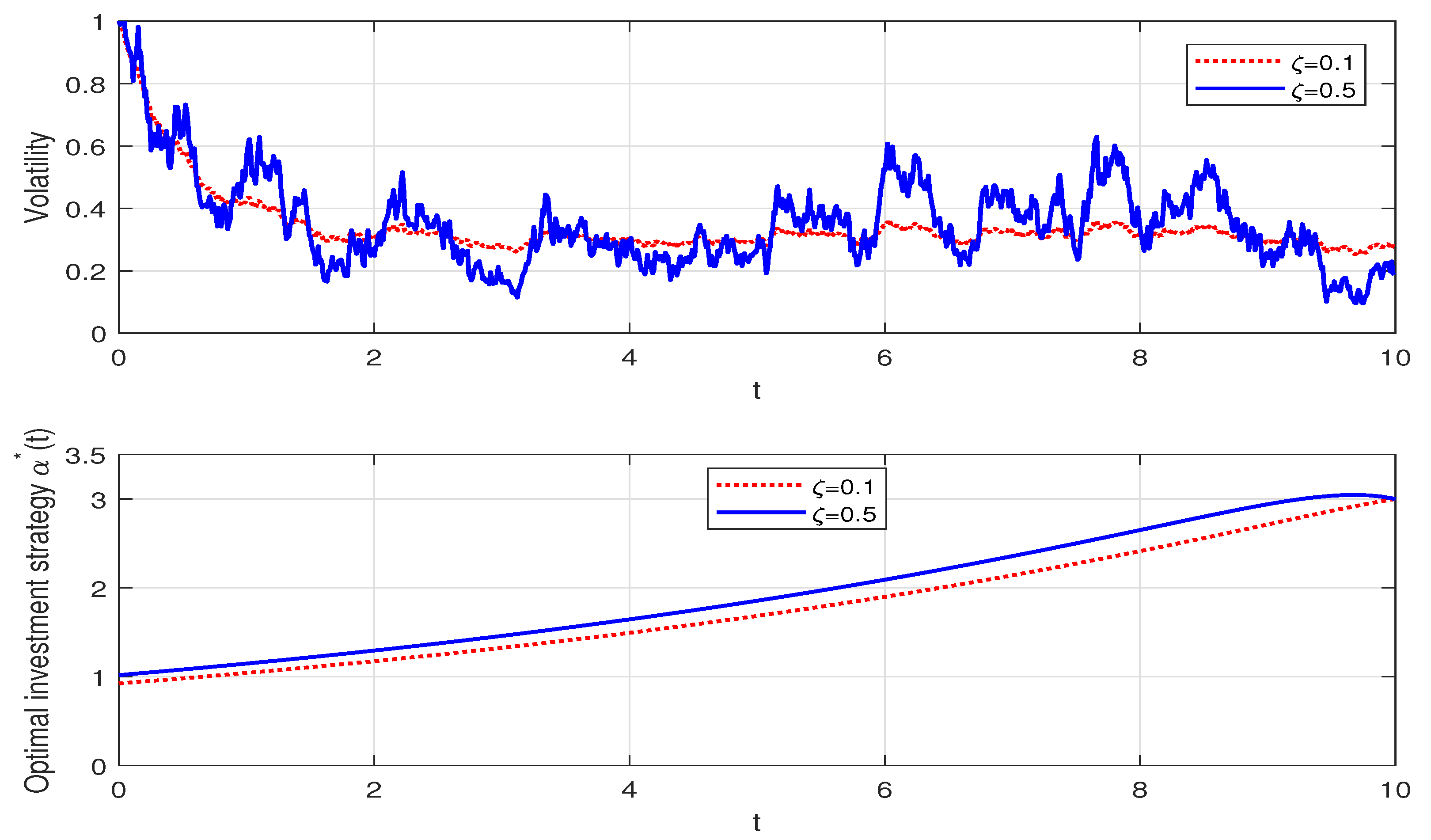
For the Heston model, represents the price volatility of the risky asset. We plot the simulation sample path of by using the Monte Carlo method. Figure 1 illustrates that a larger leads to the volatility of the risky asset, with drastic fluctuations, which is consistent with our intuition. It also can be observed that increases with regard to . When , a greater degree of volatility leads to the expected increase in the risky asset’s price. Therefore, with the increase in , the insurer will allocate more in the risky asset. In addition, the optimal dollar amount invested in the risky asset increases with regard to time t. As the terminal time approaches, the insurer prefers to adopt a more conservative portfolio and will slightly decrease the portfolio in the risky asset.
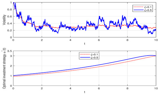
Figure 1.
The effect of on the optimal investment strategy.
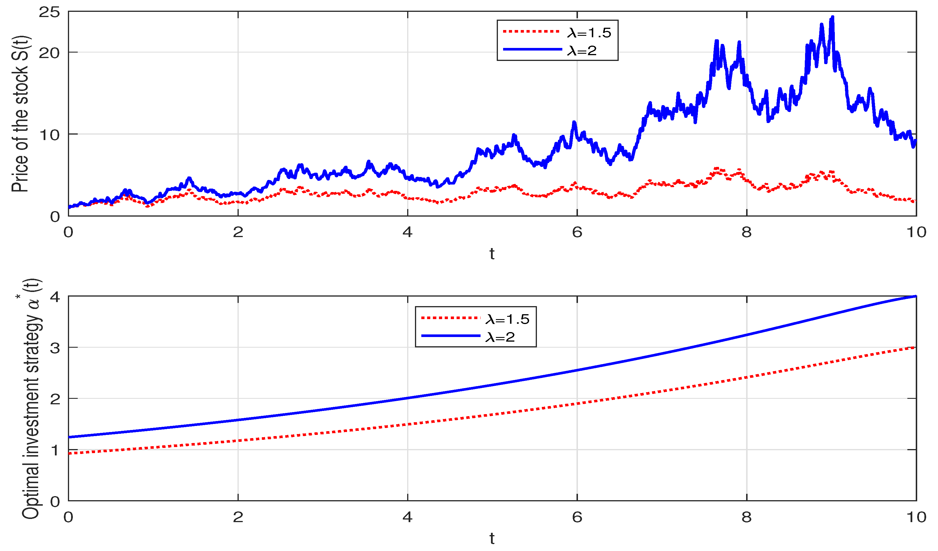
Figure 2 demonstrates the effects of on the optimal investment strategy. In fact, the appreciation rate of the risky asset increases with regard to . We observe that increases with rising, which can be attributed to a higher , indicating that the insurer will generate greater returns when they bear extra risk, leading to more investment in the risky asset.
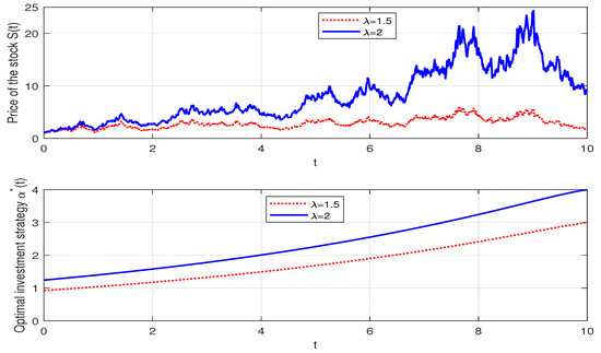
Figure 2.
The effect of on the optimal investment strategy.
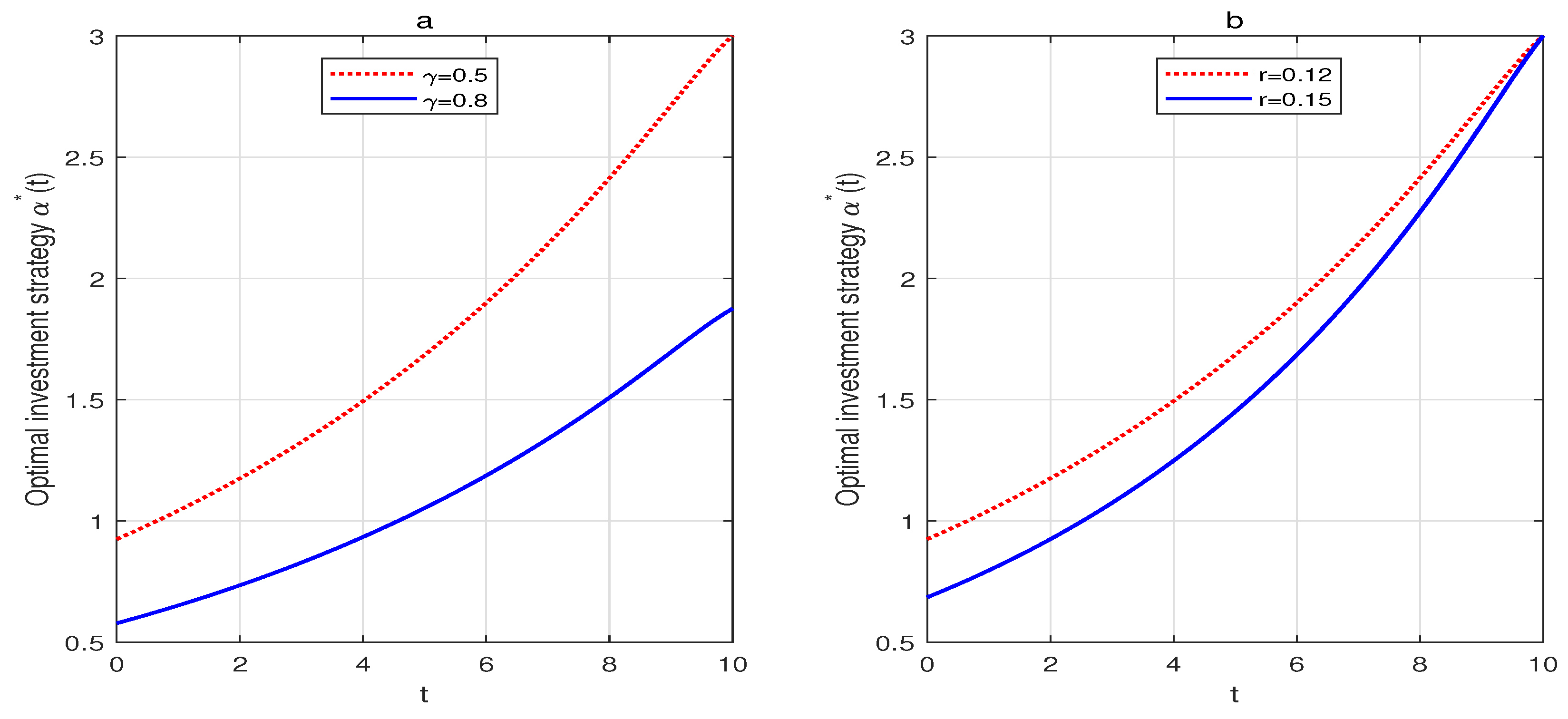
Figure 3a illustrates the effects of the risk aversion parameter on the optimal investment strategy. The negative impact of on suggests that the insurer with a higher level of risk aversion will reduce their investment in the risky asset. From Figure 3b, we can see that is a decreasing function of r. When r increases, the risk-free asset becomes more attractive, and so the insurer invests more in the risk-free asset and reduces investment in the risky asset.
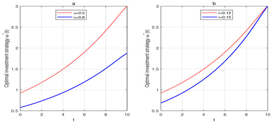
Figure 3.
(a) The effect of on the optimal investment strategy. (b) The effect of r on the optimal investment strategy.
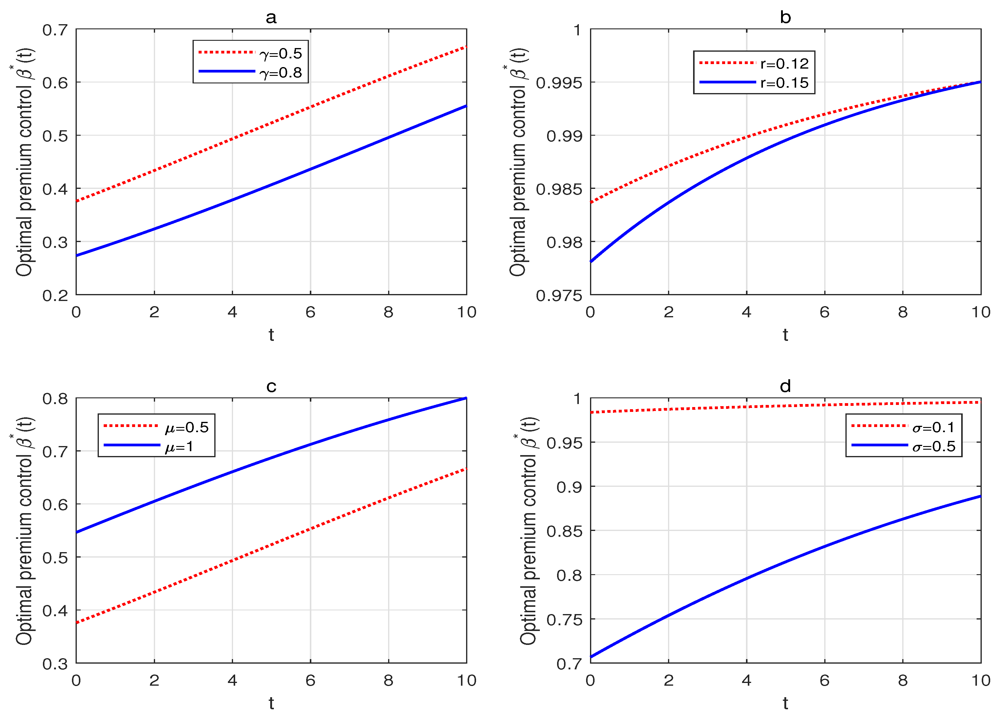
According to , it is not difficult to calculate that , , , and , which implies that the optimal premium control variable increases with regard to time t, and the expected claim amount , decreases with regard to the risk aversion parameter , the risk-free interest rate r and the volatility of claim amount . Figure 4a illustrates that the optimal premium control variable decreases as increases. Combined with the previous analysis, we conclude that has a positive relationship with the safety loading . Therefore, the more the insurer dislikes risk, the more expensive the adopted premium rate. Figure 4b depicts the negative relationship between the risk-free interest rate r and . In other words, the safety loading increases with r. This phenomenon can be interpreted as if the insurer has to loan from the money market at a higher interest rate, and thus it would be wise to raise the premium rate. In Figure 4c, the optimal premium control is an increasing function of , owing to a greater , which means a larger expected claim amount. The insurer would like to lower the premium rate to win large policy businesses. In addition, we can observe in Figure 4d that decreases with the volatility of claim amount , i.e., the insurer wishes to charge a higher premium if there is a heavy deviation among claims amount.
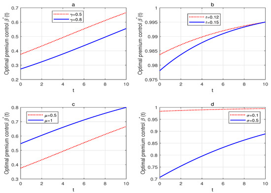
Figure 4.
(a) The effect of on the optimal premium control. (b) The effect of r on the optimal premium control. (c) The effect of on the optimal premium control. (d) The effect of on the optimal premium control.
Without the loss of generality, we provide the evolution of the optimal value functions with regard to the parameters of the insurance market at the initial time 0 and the cost rate . We define and in the optimization problem with the determined premium.
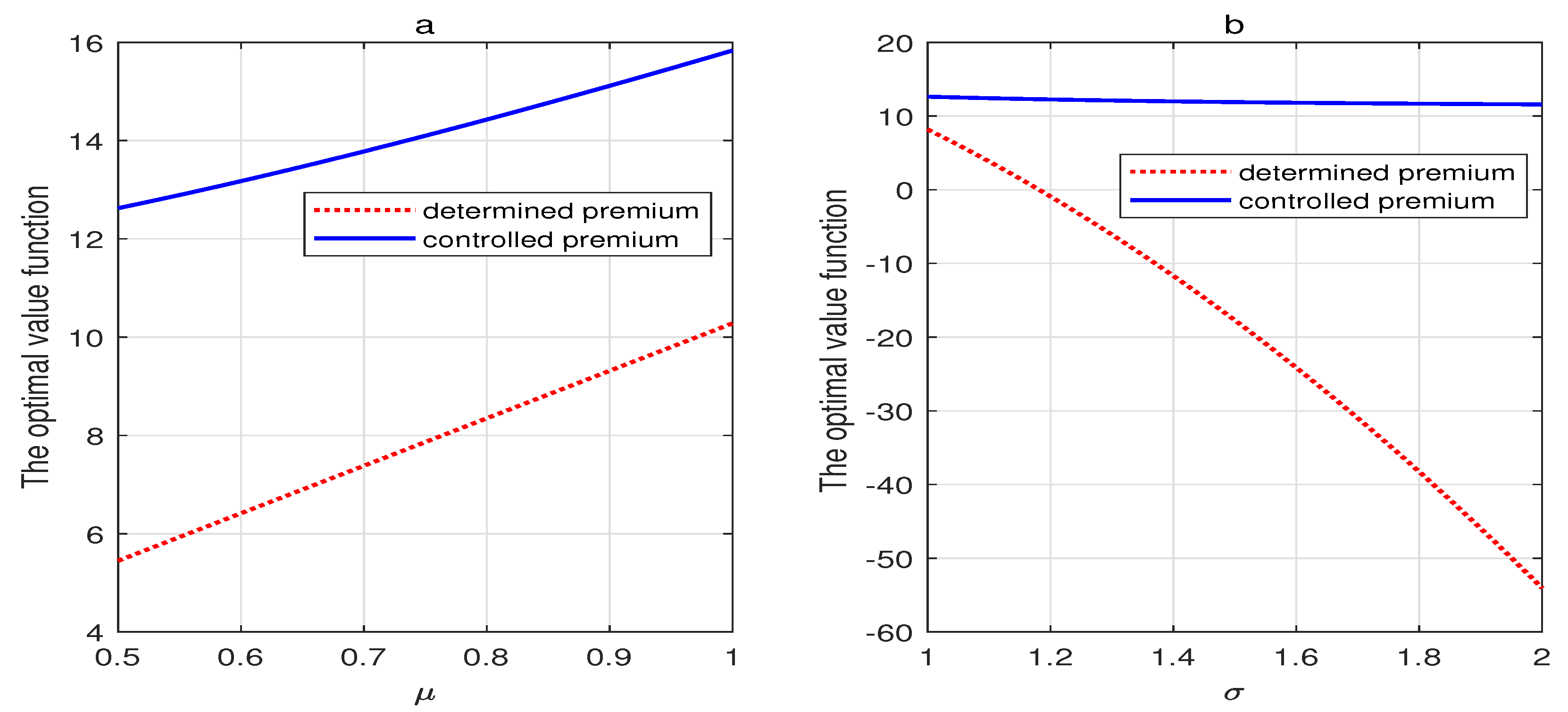
Figure 5a depicts the effect of on the optimal value functions under the traditional homogeneous Poisson model (determined premium) and the non-homogeneous Poisson model introduced here (controlled premium) . is identified as the expected claim amount, and as previously mentioned, the premium decreases with regard to . The insurer offers favorable premiums to acquire large policy bonuses, leading to a higher utility level than the determined premium case. In addition, represents the volatility of the surplus. Figure 5b shows that the two optimal value functions decrease as the volatility becomes large. The optimal value function under the controlled premium case is larger than that under the determined premium case. With the increase in the surplus’s volatility, we find that if the insurer does not adjust the premium based on the insurance market, it will incur a huge utility loss. Moreover, we conclude that the premium control mechanism will lead to higher optimal utilities, and the insurer could improve the utility by adjusting premiums flexibly.
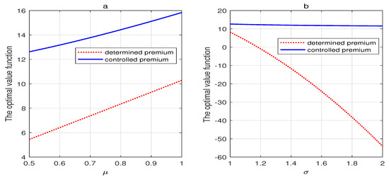
Figure 5.
(a) The effect of on the optimal value function. (b) The effect of on the optimal value function.
6. Conclusions
This paper considers the optimal investment and premium control strategies for insurers with the short-selling constraint under the mean-variance criterion. We utilize the non-homogeneous compound Poisson process containing time-varying intensity to describe the claim process. The financial market is composed of one risk-free asset and one risky asset for which the price process follows the Heston model. We construct the extended HJB equations by applying the stochastic control theory and obtain the closed-form solution for the optimization problem. In addition, numerical simulations and sensitivity analyses are provided. Unlike Zhou et al. (2017) [20] and Liu et al. (2020) [22], who investigated the optimal investment and premium control problems under expected utility theory (EUT), we studied the optimal time-consistent strategies under the mean-variance criterion.
In further research, we hope to study the optimal asset allocation problem with partial information. The assumption of complete information seems to be a common characteristic, which indicates that the insurer possesses comprehensive knowledge of the model. Nevertheless, in reality, the insurer operates in an environment with partial information. We hope to adopt a risk model with a claim arrival intensity and claim size distribution affected by an unobservable environmental stochastic factor. The classical HJB approach may not be appropriate since the filter process is infinite-dimensional, and we devote our attention to the Backward Stochastic Differential Equation (BSDE). These problems remain to be investigated in the future.
Author Contributions
Writing—review and editing, funding acquisition, and methodology, Z.L.; writing—original draft and visualization, Y.W.; supervision and validation, Y.H. and J.Z. All authors have read and agreed to the published version of the manuscript.
Funding
This research was funded by the National Social Science Foundation of China (No.20BJY264).
Institutional Review Board Statement
Not applicable.
Informed Consent Statement
Not applicable.
Data Availability Statement
Not applicable.
Acknowledgments
The authors would like to thank the editors and reviewers for their help.
Conflicts of Interest
The authors declare no conflict of interest.
Appendix A
The proof consists of two steps:
- (i)
- We show that , , is the value function corresponding to , i.e., that .For satisfying thatthen . Applying the Itô formula on ,The last term is an square-integrable martingale with zero expectation, taking the conditional expectation on both sides of the above formula, we have . Furthermore, similarly, for satisfying thatwe conclude that .For the specific admissible strategy , as is shown in (13), and satisfy thatTherefore, and .We denote , . According to the Itô formula, for , we haveand the last equation holds, due to the fact that . Using the Itô formula on ,As is mentioned in (13) that ,Substituting for , and inserting (A4) into (A6), we haveTaking expectations and supremum over givesFor a specific admissible strategy , as is mentioned in (2) of Theorem 1, we have and thusTaking the conditional expectation on both sides of the above formula results inHence, we conclude that .
- (ii)
- We prove that is indeed an equilibrium strategy.For , defined in Definition 2, we rewrite (A4) asAccording to (A6), we haveBased on the fact that in Definition 2, we obtain that . Inserting (A11) into (A12), we find thatTaking the condition expectation on both sides,which implies that .
Appendix B
The optimization objective function has the form
which deduces that
We conjecture and in the following way:
Thus, we have
Substituting (A14) into (13), we have
According to the first-order conditions, we have
Define , and is strictly increasing in because of . In addition, , .
For the investment policy, we consider that if (1) ; or (2) with , the short-selling constraint is satisfied and thus ; if and , we can judge that .
For the premium control, note that is strictly concave. If , must be strictly decreasing in , which contradicts the assumption at the end of Section 2.1, that . Therefore, we admit that and thus, we have . The strictly increasing continuous function has values of the opposite sign inside the interval , with a unique root . Next, we discuss our results in the following cases:
- Case I. .
If , we have and the short-selling constraint is satisfied. Thus, we can judge that the optimal strategies . Substituting (A16) into (A15) and separating the variables, we decompose them into the following ODEs:
If , we denote the solutions for the above ODEs (A17) by , , and ; thus
where
and if , the solutions for the above ODEs (A17) are , , and . We find that
where
In this case, the optimal strategies
and the value function is
- Case I. with .
This case possesses the same results as Case I, and we omit it here.
- Case II. with .
with means that , and the short-selling constraint fails. Then, we simply identify that . By a similar derivation to the above cases, we have
After solving the equations, we obtain the optimal policies
and the value function is .
References
- Browne, S. Optimal investment policies for a firm with a random risk process: Exponential utility and minimizing the probability of ruin. Math. Oper. Res. 1995, 20, 937–958. [Google Scholar] [CrossRef] [Green Version]
- Hipp, C.; Plum, M. Optimal investment for insurers. Insur. Math. Econ. 2000, 27, 215–228. [Google Scholar] [CrossRef]
- Schmidli, H. On minimizing the ruin probability by investment and reinsurance. Ann. Appl. Probab. 2002, 12, 890–907. [Google Scholar] [CrossRef]
- Liu, C.; Yang, H. Optimal investment for an insurer to minimize its probability of ruin. N. Am. Actuar. J. 2004, 8, 11–31. [Google Scholar] [CrossRef]
- Promislow, S.; Young, V. Minimizing the probability of ruin when claims follow Brownian motion with drift. N. Am. Actuar. J. 2005, 9, 110–128. [Google Scholar] [CrossRef]
- Bi, J.; Chen, K. Optimal investment-reinsurance problems with shock dependent risks under two kinds of premium principles. RAIRO-Oper. Res. 2019, 53, 179–206. [Google Scholar] [CrossRef] [Green Version]
- Zhang, Y.; Zhao, P. Optimal reinsurance-investment problem with dependent risks based on Legendre transform. J. Ind. Manag. Optim. 2020, 16, 1457–1479. [Google Scholar]
- Li, D.; Rong, X.; Zhao, H.; Yi, B. Equilibrium investment strategy for DC pension plan with default risk and return of premiums clauses under CEV model. Insur. Math. Econ. 2017, 72, 6–20. [Google Scholar] [CrossRef]
- Xiao, H.; Ren, T.; Bai, Y.; Zhou, Z. Time-consistent investment-reinsurance strategies for the insurer and the reinsurer under the generalized mean-variance criteria. Mathematics 2019, 7, 857. [Google Scholar] [CrossRef] [Green Version]
- Yuan, Y.; Mi, H.; Chen, H. Mean-variance problem for an insurer with dependent risks and stochastic interest rate in a jump-diffusion market. Optimization 2021. [Google Scholar] [CrossRef]
- Markowitz, H. Portfolio selection. J. Financ. 1952, 7, 77–91. [Google Scholar]
- Strotz, R. Myopia and inconsistency in dynamic utility maximization. Rev. Econ. Stud. 1955, 23, 165–180. [Google Scholar] [CrossRef]
- Zhou, X.; Li, D. Continuous-time mean-variance portfolio selection: A stochastic LQ framework. Appl. Math. Opt. 2000, 42, 19–33. [Google Scholar] [CrossRef]
- Li, D.; Ng, W. Optimal dynamic portfolio selection: Multiperiod mean-variance formulation. Math. Financ. 2000, 10, 387–406. [Google Scholar] [CrossRef]
- Björk, T.; Murgoci, A. A general theory of Markovian time inconsistent stochastic control problems. SSRN 2010. [Google Scholar] [CrossRef] [Green Version]
- Zeng, Y.; Li, Z. Optimal time-consistent investment and reinsurance policies for mean-variance insurers. Insur. Math. Econ. 2011, 49, 145–154. [Google Scholar] [CrossRef]
- Li, Y.; Li, Z. Optimal time-consistent investment and reinsurance strategies for mean-variance insurers with state dependent risk aversion. Insur. Math. Econ. 2013, 53, 86–97. [Google Scholar] [CrossRef]
- Bai, Y.; Zhou, Z.; Gao, R.; Xiao, H. Nash equilibrium investment-reinsurance strategies for an insurer and a reinsurer with intertemporal restrictions and common interests. Mathematics 2020, 8, 139. [Google Scholar] [CrossRef] [Green Version]
- Wang, N.; Zhang, N.; Jin, Z.; Qian, L. Reinsurance-investment game between two mean-variance insurers under model uncertainty. J. Comput. Appl. Math. 2021, 382, 113095. [Google Scholar] [CrossRef]
- Zhou, M.; Yuen, K.; Yin, C. Optimal investment and premium control for insurers with a nonlinear diffusion model. Acta Math. Appl. Sin.-E 2017, 33, 945–958. [Google Scholar] [CrossRef] [Green Version]
- Jiang, X.; Yuen, K.; Chen, M. Optimal investment and reinsurance with premium control. J. Ind. Manag. Optim. 2020, 16, 2781–2797. [Google Scholar] [CrossRef]
- Liu, B.; Zhou, M.; Li, P. Optimal investment and premium control for insurers with ambiguity. Commun. Stat.-Theor. Methods 2020, 49, 2110–2130. [Google Scholar] [CrossRef]
- Beckers, S. The constant elasticity of variance model and its implications for option pricing. J. Financ. 1980, 35, 661–673. [Google Scholar] [CrossRef]
- Hobson, D.; Rogers, L. Complete models with stochastic volatility. Math. Financ. 1998, 8, 27–48. [Google Scholar] [CrossRef]
- Taylor, S. Financial returns modeled by the product of two stochastic processes, a study of daily sugar prices 1961–75. In Time Series Analysis: Theory and Practice; Anderson, O., Ed.; North-Holland Publishing Company: Amsterdam, The Netherlands, 1982; pp. 203–226. [Google Scholar]
- Cox, J.; Ross, S. The valuation of options for alternative stochastic processes. J. Financ. Econ. 1976, 3, 145–166. [Google Scholar] [CrossRef]
- Hull, J.; White, A. The pricing of options on assets with stochastic volatilities. J. Financ. 1987, 42, 281–300. [Google Scholar] [CrossRef]
- Heston, S. A closed-form solution for options with stochastic volatility with applications to bond and currency options. Rev. Financ. Stud. 1993, 6, 327–343. [Google Scholar] [CrossRef] [Green Version]
- Li, Z.; Zeng, Y.; Lai, Y. Optimal time-consistent investment and reinsurance strategies for insurers under Heston’s SV model. Insur. Math. Econ. 2012, 51, 191–203. [Google Scholar] [CrossRef]
- Lin, X.; Qian, Y. Time-consistent mean-variance reinsurance-investment strategy for insurers under CEV model. Scand. Actuar. J. 2016, 2016, 646–671. [Google Scholar] [CrossRef]
- Zhu, H.; Cao, M.; Zhang, C. Time-consistent investment and reinsurance strategies for mean-variance insurers with relative performance concerns under the Heston model. Financ. Res. Lett. 2019, 30, 280–291. [Google Scholar] [CrossRef]
- Luo, S.; Taksar, M.; Tsoi, A. On reinsurance and investment for large insurance portfolios. Insur. Math. Econ. 2008, 42, 434–444. [Google Scholar] [CrossRef]
- Bai, L.; Guo, J. Optimal proportional reinsurance and investment with multiple risky assets and no-shorting constraint. Insur. Math. Econ. 2008, 42, 968–975. [Google Scholar] [CrossRef]
- Liu, S.; Zhang, J. Optimal investment and excess of loss reinsurance with short-selling constraint. Acta. Math. Appl. Sin.-E 2011, 27, 527–534. [Google Scholar] [CrossRef]
- Bi, J.; Guo, J. Optimal mean-variance problem with constrained controls in a jump-diffusion financial market for an insurer. J. Optim. Theory Appl. 2013, 157, 252–275. [Google Scholar] [CrossRef]
- Huang, Y.; Yang, X.; Zhou, J. Optimal investment and proportional reinsurance for a jump-diffusion risk model with constrained control variables. J. Comput. Appl. Math. 2016, 296, 443–461. [Google Scholar] [CrossRef]
- Grandell, J. Finite time ruin probabilities and martingales. Informica 1991, 2, 3–32. [Google Scholar]
- Zhao, H.; Rong, X.; Zhao, Y. Optimal excess-of-loss reinsurance and investment problem for an insurer with jump-diffusion risk process under the Heston model. Insur. Math. Econ. 2013, 53, 504–514. [Google Scholar] [CrossRef]
- Eraker, B.; Johannes, M.; Polson, N. The impact of jumps in volatility and returns. J. Financ. 2003, 58, 1269–1300. [Google Scholar] [CrossRef]
Publisher’s Note: MDPI stays neutral with regard to jurisdictional claims in published maps and institutional affiliations. |
© 2022 by the authors. Licensee MDPI, Basel, Switzerland. This article is an open access article distributed under the terms and conditions of the Creative Commons Attribution (CC BY) license (https://creativecommons.org/licenses/by/4.0/).

