Communication-Efficient Distributed Learning for High-Dimensional Support Vector Machines

Abstract

Distributed learning has received increasing attention in recent years and is a special need for the era of big data. For a support vector machine (SVM), a powerful binary classification tool, we proposed a novel efficient distributed sparse learning algorithm, the communication-efficient surrogate likelihood support vector machine (CSLSVM), in high-dimensions with convex or nonconvex penalties, based on a communication-efficient surrogate likelihood (CSL) framework. We extended the CSL for distributed SVMs without the need to smooth the hinge loss or the gradient of the loss. For a CSLSVM with lasso penalty, we proved that its estimator could achieve a near-oracle property for $l_1$ penalized SVM estimators on whole datasets. For a CSLSVM with smoothly clipped absolute deviation penalty, we showed that its estimator enjoyed the oracle property, and that it used local linear approximation (LLA) to solve the optimization problem. Furthermore, we showed that the LLA was guaranteed to converge to the oracle estimator, even in our distributed framework and the ultrahigh-dimensional setting, if an appropriate initial estimator was available. The proposed approach is highly competitive with the centralized method within a few rounds of communications. Numerical experiments provided supportive evidence.

1. Introduction

The support vector machine (SVM), originally introduced by [1], has been a great success when applied to many classification problems. Owing to its high accuracy and flexibility it has provided solid mathematical foundations in machine learning. It is one of the most popular binary classification tools. The motivation of an SVM is to find a maximum-margin hyperplane by a regularized functional optimization problem. In statistical machine learning, the penalized functional is a sum of the hinge loss plus $l_2$-norm regularization. The statistical properties of an SVM have been studied in a lot of works. In this work, we focused on a distributed penalized linear SVM for datasets with large sample sizes and large dimensions.

With the development of modern technology, the size of data has become incredibly large, and, in some cases, cannot even be stored on a single machine. In real-world applications, many datasets are stored locally on individual servers and individual’s devices, such as mobile phones and computers. It is difficult to collect these local data onto a single machine due to communication costs and privacy preservation. Thus, new methods and theories in distributed learning are called for. Distributed learning has attracted increasing attention in recent years, for example, see Refs. [2,3] for M-estimation, Refs. [4,5,6] for quantile regression, Refs. [7,8] for nonparametric regression, Refs. [3,9] for confidence intervals, and so on. These works focus on the simple setting of data parallelism under which the dataset is partitioned and distributed on m worker machines that can analyze data independently. Most methods suggest that in each round of communication, each worker machine estimates the parameters of the model locally, and then communicates these local estimators to a master machine that averages these estimators to form a global estimator. Although this divide-and-conquer approach is communication-efficient, it has some restrictions: for achieving the minimax rate of convergence, the number of worker machines cannot be too large and samples in each worker machine should be large enough, these restrictions are highly restrictive. In addition, averaging can perform poorly if the estimator is nonlinear.

Not only can the size of data be exceedingly large, but also many successful models are heavily over-parameterized. These problems have been discussed widely. Zou [10] proposed an improved $l_1$ penalized SVM for simultaneous feature selection and classification, and showed that the hybrid SVM not only often improved the classification accuracy, but also enjoyed better feature-selection performance. Meinshausen and Buhlmann [11] studied the problem of variable selection in high-dimensional graphs, and explained that neighborhood selection with the lasso is a computationally attractive alternative to standard covariance selection for sparse high-dimensional graphs. Zhao and Yu [12] studied almost necessary and sufficient conditions for lasso to select the true model when $p<n$ or $p\gg n$, where p was the dimension of the model parameters and n was the sample size. Meinshausen and Yu [13] introduced sparse representations for high-dimensional data and proved that the estimator was still consistent even though the lasso could not recover the correct sparsity pattern. The adaptive lasso was proposed by Zou [14] and is a new version of the lasso that enjoys oracle properties. In the high-dimensional problems, the dimension p of the covariates was larger than the size of data, but there were only a few covariates that were relevant to the response. As a concrete example, in a microarray data set, which contains more than 10,000 genes, only several genes will make a difference to the result. Recently, the statistical inference for high-dimensional data has been investigated; readers can refer to [15,16] for details. In high-dimensional surroundings, a standard SVM can be easily affected by many redundant variables, so variable selection is important for high-dimensional SVMs. Fan and Fan [17] has shown that it was as poor as “tossing a coin” if all features were used in classification due to the accumulation of noise in high-dimensional analysis. Many works have been proposed to handle such a problem. Bradley and Mangasarian [18], Peng et al. [19], Zhu et al. [20] and Wegkamp and Yuan [21] studied the $l_1$ penalized SVM; Fan and Li [22] proposed an approach of variable selection and the estimation of model simultaneously by using a smoothly clipped absolute deviation penalty (SCAD) or minimax concave penalty (MCP), which are non-convex. Becker et al. [23], Park et al. [24] and Zhang et al. [25] considered the SCAD penalized SVM. Lian and Fan [26] gave the divide-and-conquer debiased estimator for an SVM, but such simple averaging might result in high computational costs for the high-dimensional problem, although it could become a debiased estimator by the lasso penalty. Jordan et al. [3] proposed the communication-efficient surrogate likelihood (CSL) framework for solving distributed statistical inference problems, which could work for high-dimensional penalized regression. As [27] stated, the CSL approach is different from distributed first-order optimization methods, which leverage both global first-order information and local higher-order information; yet, to the best of our knowledge, the distributed inference of variable selection for high-dimensional SVM has not been studied in the CSL framework.

In this paper, we propose communication-efficient distributed learning for support vector machines in high dimensions. Instead of using all the data to estimate the parameters, our method only needed to solve a regularized optimization problem on the first machine that was based on all gradients obtained from all worker machines. For the penalty function, we considered the convex $l_1$ and the non-convex SCAD penalty in a high-dimensional SVM, which could achieve variable selection and estimation simultaneously. In the distributed learning high-dimensional SVM, we did not need smooth assumptions to the loss or the gradient of the loss. We give some theoretical results in the paper.

The reminder of this paper is organized as follows. In Section 2, we give the problem formulation. Communication-efficient distributed estimation for an SVM is presented in Section 3. In Section 4, we provide simulation studies and real data examples and demonstrate encouraging performances.

2. Problem Formulation

In this section, we set up our learning problem formally. We considered a strategy, which was empirical risk minimization, to obtain the optimal model. We considered a distributed learning framework with m worker machines, in which the 1st machine was regarded as the central machine. The 1st worker could aggregate information from another $m-1$ worker machines. In addition, every machine had n samples. So the size of total samples was $N=nm$. For a standard binary classification problem, we denoted $\mathcal{X}$ to be the input space and $\mathcal{Y}=\{-1,+1\}$ to be the output space. Random vectors $(\mathit{X},\mathit{Y})\in \mathcal{X}\times \mathcal{Y}$ were drawn from an unknown joint distribution $\mathcal{D}$ on $\mathcal{X}\times \mathcal{Y}$. Let the parameters $\mathbf{\beta }={\left({\beta }_0,{\beta }_1,\dots ,{\beta }_p\right)}^{\mathrm{T}}$ and the features ${\mathbf{x}}_i={\left(1,x_{i1},\dots ,x_{ip}\right)}^{\mathrm{T}}$. Suppose that training data points ${\left\{\left({\mathbf{x}}_i,y_i\right)\right\}}_{i=1}^N$ are available from $\mathcal{D}$. Let $\ell \left(\mathit{X},\mathbf{\beta }\right)$ be a loss function and

$${\mathbf{\beta }}_0=arg\underset{\beta }{min}\mathrm{E}\ell \left(\mathit{X},\mathbf{\beta }\right),$$

where ${\mathbf{\beta }}_0={\left({\beta }_{00},{\beta }_{01},\dots ,{\beta }_{0p}\right)}^{\mathrm{T}}$ is the true parameter. Let the i.i.d (independent identically distributed) samples ${\left\{\left({\mathbf{x}}_i,y_i\right)\right\}}_{i=1}^N$ be stored on m machines and use ${\mathcal{I}}_k$ to denote the indices of samples on the kth machine with $\left|{\mathcal{I}}_k\right|=n=N/m$ for all $k\in \left[m\right]$ and ${\mathcal{I}}_j\cap {\mathcal{I}}_k=\varnothing \mathrm{for}j\ne k$, $j,k\in \left[m\right]$. The empirical risk of the kth machine is defined by

$${\widehat{L}}_k\left(\mathbf{\beta }\right)=\frac{1}{\left|{\mathcal{I}}_k\right|}\sum _{i\in {\mathcal{I}}_k}\ell \left(\mathbf{\beta };({\mathit{X}}_i,y_i)\right),$$

the empirical risk based on all N samples is

$$\widehat{L}\left(\mathbf{\beta }\right)=\frac{1}{m}\sum _{k=1}^m{\widehat{L}}_k\left(\mathbf{\beta }\right).$$

We used structural risk minimization strategy to learn ${\mathbf{\beta }}_0$, which is defined by

$$\widehat{\mathbf{\beta }}={argmin}_{\beta }\{\widehat{L}\left(\beta \right)+g\left(\beta \right)\},$$

where $g\left(\mathbf{\beta }\right)$ is the penalty term, such as $l_1$, $l_2$, SCAD and MCP.

In distributed statistical learning, Jordan et al. [3] proposed a distributed estimator with statistical guarantee and communication efficiency. Given an appropriate initial estimator $\tilde{\mathbf{\beta }}$, we have

$$\tilde{L}\left(\mathbf{\beta }\right)={\widehat{L}}_1\left(\mathbf{\beta }\right)-{\mathbf{\beta }}^{\mathrm{T}}\left(\nabla {\widehat{L}}_1\left(\tilde{\mathbf{\beta }}\right)-\nabla \widehat{L}\left(\tilde{\mathbf{\beta }}\right)\right).$$

By the above formula, we could introduce a communication-efficient distributed learning algorithm: the first worker machine broadcasts the initial $\tilde{\mathbf{\beta }}={\widehat{\mathbf{\beta }}}_1$ to the remaining $m-1$ machines and each machine computes the local gradient $\nabla {\widehat{L}}_k\left(\tilde{\mathbf{\beta }}\right)$. Then, these local gradients are sent back to the first machine where the first worker carries out an SVM by aggregating these local gradients. The communication-efficient estimator is given by

$$\check{\mathbf{\beta }}={argmin}_{\mathbf{\beta }}\{\tilde{L}\left(\mathbf{\beta }\right)+g\left(\mathbf{\beta }\right)\},$$

with approximate loss $\tilde{L}\left(\mathbf{\beta }\right)$. The architecture of the distributed learning reduced the total communication costs $O\left(\right(m-1\left)np\right)$ to $O\left(\right(m-1\left)p\right)$, where p is the dimension of $\mathbf{\beta }$.

3. Distributed Learning for an SVM

A standard non-separable SVM has the following form,

$$\widehat{L}\left(\mathbf{\beta }\right)+g\left(\mathbf{\beta }\right)=\frac{1}{N}\sum _{i=1}^N{\left(1-y_i{\mathit{X}}_i^{\mathrm{T}}\mathbf{\beta }\right)}_{+}+\frac{\lambda }{2}{\parallel {\mathbf{\beta }}^{*}\parallel }_2^2,$$

where ${\left(x\right)}_{+}=max\left(x,0\right)$ is the hinge loss function that is piecewise linear and is differentiable except at point 0; ${\mathbf{\beta }}^{*}={\left({\beta }_1,\dots ,{\beta }_p\right)}^{\mathrm{T}}$ is the unknown p-dimensional parameter; $\lambda$ is the regularization parameter, which determines the importance of penalty term. The true parameter ${\mathbf{\beta }}_0$ is the minimum of the following population loss function

$$L\left(\mathbf{\beta }\right)=\mathrm{E}{\left[1-Y{\mathit{X}}^{\mathrm{T}}\mathbf{\beta }\right]}_{+}.$$

We define

$$S\left(\mathbf{\beta }\right)=-\mathrm{E}\left\{I\left(1-Y{\mathit{X}}^{\mathrm{T}}\mathbf{\beta }⩾0\right)Y\mathit{X}\right\},$$

$$H\left(\mathbf{\beta }\right)=\mathrm{E}\left\{\delta \left(1-Y{\mathit{X}}^{\mathrm{T}}\mathbf{\beta }\right)\mathit{X}{\mathit{X}}^{\mathrm{T}}\right\},$$

where $I\left\{·\right\}$ is the indicator function and $\delta \left\{·\right\}$ is the Dirac delta function. The $S\left(\mathbf{\beta }\right)$ and $H\left(\mathbf{\beta }\right)$ could be viewed as the gradient vector and Hessian matrix of $L\left(\mathbf{\beta }\right)$.

The empirical loss function of the kth worker machine is ${\widehat{L}}_k\left(\mathbf{\beta }\right)=\frac{1}{\left|{\mathcal{I}}_k\right|}{\sum }_{i\in {\mathcal{I}}_k}{\left(1-y_i{\mathit{X}}_i^{\mathrm{T}}\mathbf{\beta }\right)}_{+}.$ Given $\tilde{\mathbf{\beta }}$ is an initial estimator of ${\mathbf{\beta }}_0$, we use $\tilde{L}\left(\mathbf{\beta }\right):={\widehat{L}}_1\left(\mathbf{\beta }\right)-{\mathbf{\beta }}^{\mathrm{T}}\left(\nabla {\widehat{L}}_1\left(\tilde{\mathbf{\beta }}\right)-\nabla \widehat{L}\left(\tilde{\mathbf{\beta }}\right)\right)$ to replace $\widehat{L}\left(\mathbf{\beta }\right)=\frac{1}{N}{\sum }_{i=1}^N{\left(1-y_i{\mathit{X}}_i^{\mathrm{T}}\mathbf{\beta }\right)}_{+}$, and then obtain the distributed estimator

$$\check{\mathbf{\beta }}=\underset{\mathbf{\beta }}{argmin}\tilde{L}\left(\mathbf{\beta }\right)+g\left(\mathbf{\beta }\right).$$

(1)

In this paper, we considered the $l_1$ penalty and SCAD penalty, respectively. The $l_1$ penalty is

$$g\left(\mathbf{\beta }\right)={\lambda \parallel \mathbf{\beta }\parallel }_1,$$

and the SCAD penalty is

$$g\left(\mathbf{\beta }\right)=\sum _{j=1}^p{p}_{\lambda }\left(\left|{\mathbf{\beta }}_j\right|\right),$$

where

$$\begin{array}{ccc}\hfill p_{\lambda }\left(t\right)& =& \lambda \left|t\right|I(0⩽\left|t\right|<\lambda )+\frac{a\lambda \left|t\right|-\left(t^2+{\lambda }^2\right)/2}{a-1}I(\lambda ⩽|t|⩽a\lambda )\hfill \\ & & +\frac{(a+1){\lambda }^2}{2}I\left(\right|t|>a\lambda )\hfill \end{array}$$

for some $a>2$. Note that the SCAD penalty has the following properties:

Property 1: $p_{\lambda }\left(t\right)$ is symmetric and for $t\in \left[0,\infty \right)$ is non-decreasing and concave, with $p_{\lambda }\left(0\right)=0$.

Property 2: The derivative of $p_{\lambda }\left(t\right)$ is continuous on $\left(0,\infty \right)$: for some $a>1$,

${lim}_{t\to 0+}{p}_{\lambda }^{\prime }\left(t\right)$$=\lambda$, $p_{\lambda }^{\prime }\left(t\right)⩾\lambda -t/a$ for $0<t<a$, and $p_{\lambda }^{\prime }\left(t\right)=0$ for $t⩾a\lambda$.

In practice, we adopted the following CSL distributed learning for an SVM, which is summarized in Algorithm 1. However, our theories were based on the distributed estimator $\check{\mathbf{\beta }}$ in (1).

Algorithm 1: CSL distributed support vector machine (CSLSVM).

3.1. A Communication-Efficient Distributed SVM with Lasso Penalty

In this section, we establish the theoretical properties of the proposed estimator. Despite the generality and elegance of [3]’s method, the approach uses only at least second derivatives for smooth loss functions, such as cross-entropy loss, which can not directly apply to the hinge loss of an SVM. Recall that surrogate loss $\tilde{L}\left(\mathbf{\beta }\right):={\widehat{L}}_1\left(\mathbf{\beta }\right)-{\mathbf{\beta }}^{\mathrm{T}}\left(\nabla {\widehat{L}}_1\left(\tilde{\mathbf{\beta }}\right)-\nabla \widehat{L}\left(\tilde{\mathbf{\beta }}\right)\right)$. We only used first-order information, so if the gradient existed almost everywhere, it was usable for the aforementioned method. For an SVM, the hinge loss was differentiable except at point 0. We could use a subgradient function

$$\nabla \widehat{L}\left(\mathbf{\beta }\right)=-\frac{1}{\left|{\mathcal{I}}_k\right|}\sum _{i\in {\mathcal{I}}_k}I\left(1-y_i{\mathbf{x}}_i^T\mathbf{\beta }\ge 0\right)y_i{\mathbf{x}}_i$$

in place of the gradient and, thus, the surrogate loss was directly usable.

Our main results were established under the following assumptions.

(A1) The conditional densities of ${\mathit{X}}^T{\mathbf{\beta }}_{\mathbf{01}}$ given $\mathbf{Y}=1$ and $\mathbf{Y}=-1$ are denoted as f and g, respectively. It is assumed that f is uniformly bounded away from 0 and ∞ in a neighborhood of 1, and g is uniformly bounded away from 0 and ∞ in a neighborhood of $-1$.

(A2) ${\mathbf{\beta }}_0$ is a sparse and nonzero vector, and S denotes the support of ${\mathbf{\beta }}_0$.

(A3) $\mathbf{x}$ is a sub-Gaussian random vector. That is, for any $\eta \in {\mathbb{R}}^p$,

$$E\left[exp\left\{{\eta }^{\mathrm{T}}\mathit{X}\right\}\right]\le exp\left\{{C\parallel \eta \parallel }^2\right\};$$

it is assumed that each component $x_{ij}$ of feather $x_i$ is a random variable with a mean of zero and variance 1.

Denote $\mathcal{X}={\left({\mathbf{X}}_1,{\mathbf{X}}_2,\dots ,{\mathbf{X}}_n\right)}^T$ to be the feature design matrix and define restricted eigenvalues as follows,

$${\lambda }_{max}=\underset{\delta \in {\mathbb{R}}^{p+1}:{\parallel \delta \parallel }_0\le Cq}{max}\frac{{\delta }^T{\mathcal{X}}^T\mathcal{X}\delta }{{n\parallel \delta \parallel }_2^2},$$

and

$${\lambda }_{min}\left(H\left({\mathbf{\beta }}^{*}\right);q\right)=\underset{\delta \in \Delta }{min}\frac{{\delta }^{T}H\left({\mathbf{\beta }}^{*}\right)\delta }{{\parallel \delta \parallel }_2^2},$$

where $\Delta$ is a restricted cone in ${\mathbb{R}}^{p+1}$,

$$\Delta =\left\{\gamma \in {\mathbb{R}}^{p+1}:{∥{\gamma }_{S_{+}}∥}_1\le 3{∥{\gamma }_{S_{+}^c}∥}_1\right\},$$

$S_{+}=S\cup \left\{0\right\}$, $S\subset \{1,2,\dots ,p\}$ and $\left|S\right|\le q$.

(A4) ${\lambda }_{max}$ and ${\lambda }_{min}$ are bounded away from zero.

(A5) The initial estimator $\tilde{\mathbf{\beta }}$ is sparse and ${∥\tilde{\mathbf{\beta }}-{\mathbf{\beta }}_0∥}_1\le Cq\sqrt{\frac{logp}{n}}$.

Remark 1.

Under Assumption (A1), the Hessian matrix $H\left(\mathbf{\beta }\right)$ was well-defined and continuous in β. (A1) ensured that we could obtain sufficient information around the non-differentiable point of the hinge loss; see more details in [24,28]. (A2) is a common assumption in high-dimensional problems and we knew $\left|S\right|\le s$ for some $s\le min\left\{p,n\right\}$. In this paper, we used q as the number of nonzero entries in ${\mathbf{\beta }}_0$. Using the sub-Gaussianity assumption (A3), we easily obtained ${max}_i{∥{\mathbf{x}}_i∥}_{\infty }\le C\sqrt{logp}$ with probability $1-p^{-C}$. Assumption (A4) is similar to Lemma 2 in [19]; we used these to control the bounds of the empirical loss function of the SVM and it’s expectation. (A5) is an assumption of the initial estimator for the iterative algorithm; Ref. [19] proved that the $L_1$-norm SVM coefficients satisfied such assumptions.

Our results were as follows.

Theorem 1.

Assume that (A1)–(A5) above and that $\lambda \ge 2{∥\nabla \tilde{L}\left({\mathbf{\beta }}_0\right)∥}_{\infty }$, we have with probability at least $1-n^{-C}$,

$$∥\check{\mathbf{\beta }}-{\mathbf{\beta }}_0∥\le C\left[\lambda \sqrt{q}+{\displaystyle \frac{q^{3/2}{(logp)}^{5/2}}{n}}+{\displaystyle \frac{{(qlogp)}^{1/2}}{n^{1/2}}}+{\displaystyle \frac{q^{3/2}logp}{n^{3/4}}}\right].$$

Remark 2.

Although N did not appear in the formula, in fact, the condition $\lambda \ge 2{∥\nabla \tilde{L}\left({\mathbf{\beta }}_0\right)∥}_{\infty }$ implied that the convergence rate was dependent on N. If m was not too big, that is, n was not too small, we chose $\lambda \simeq \sqrt{logp/N}$. If $q\gtrsim n^{1/4}/{(logp)}^{1/2}$ and $qlogp/n^{3/4}\lesssim \sqrt{logp/N}$, the convergence rate would be dominated by the first term $\lambda \sqrt{q}$. That is,

$$∥\check{\mathbf{\beta }}-{\mathbf{\beta }}_0∥\le C\sqrt{{\displaystyle \frac{qlogp}{N}}}.$$

This was a near-oracle property for the $l_1$ penalized SVM estimator based on the entirety of the datasets [27].

Proof of Theorem  1.

We prove the result by the following three steps in line with the proof of [6].

Step 1. Let $\delta =\check{\mathbf{\beta }}-{\mathbf{\beta }}_0.$ Since $\tilde{L}\left(\mathbf{\beta }\right)$ is convex in $\mathbf{\beta }$, we have

$$\tilde{L}\left(\mathbf{\beta }\right)-\tilde{L}\left({\mathbf{\beta }}_0\right)\ge \nabla \tilde{L}\left({\mathbf{\beta }}_0\right)\left(\mathbf{\beta }-{\mathbf{\beta }}_0\right)$$

for all $\mathbf{\beta }$. In terms of $\tilde{L}\left(\check{\mathbf{\beta }}\right)+\lambda {\parallel \check{\mathbf{\beta }}\parallel }_1\le \tilde{L}\left({\mathbf{\beta }}_0\right)+\lambda {∥{\mathbf{\beta }}_0∥}_1$ and Hölder’s inequality, we obtain

$$-{∥\nabla \tilde{L}\left({\mathbf{\beta }}_0\right)∥}_{\infty }{\parallel \delta \parallel }_1\le \tilde{L}\left(\check{\mathbf{\beta }}\right)-\tilde{L}\left({\mathbf{\beta }}_0\right)\le \lambda {∥{\mathbf{\beta }}_0∥}_1-\lambda {∥{\mathbf{\beta }}_0+\delta ∥}_1.$$

Using $\lambda \ge 2{∥\nabla \tilde{L}\left({\mathbf{\beta }}_0\right)∥}_{\infty }$, we obtain

$$-\frac{\lambda }{2}{\parallel \delta \parallel }_1\le \lambda {∥{\mathbf{\beta }}_0∥}_1-\lambda {∥{\mathbf{\beta }}_0+\delta ∥}_1.$$

Writing ${\parallel \delta \parallel }_1={∥{\delta }_S∥}_1+{∥{\delta }_{S^c}∥}_1$, ${∥{\mathbf{\beta }}_0∥}_1={∥{\mathbf{\beta }}_{0S}∥}_1$ and ${∥{\mathbf{\beta }}_0+\delta ∥}_1={∥{\mathbf{\beta }}_{0S}+{\delta }_S∥}_1+$${∥{\delta }_{S^c}∥}_1$, we obtain

$$-\frac{\lambda }{2}{∥{\delta }_S∥}_1-\frac{\lambda }{2}{∥{\delta }_{S^c}∥}_1\le \lambda {∥{\delta }_S∥}_1-\lambda {∥{\delta }_{S^c}∥}_1.$$

After rearranging, we have

$${∥{\delta }_{S^c}∥}_1\le 3{∥{\delta }_S∥}_1.$$

Step 2. We observe that

$$\begin{array}{ccc}\hfill & & \tilde{L}\left({\mathbf{\beta }}_0+\delta \right)-\tilde{L}\left({\mathbf{\beta }}_0\right)-{\delta }^{\mathrm{T}}\nabla \tilde{L}\left({\mathbf{\beta }}_0\right)={\widehat{L}}_1\left({\mathbf{\beta }}_0+\delta \right)-{\widehat{L}}_1\left({\mathbf{\beta }}_0\right)-{\delta }^{\mathrm{T}}\nabla {\widehat{L}}_1\left({\mathbf{\beta }}_0\right)\hfill \\ & =& {\displaystyle \frac{1}{n}}\sum _{i=1}^n\left(1-y_i{x}_i^T({\mathbf{\beta }}_0+\mathbf{\delta })\right)I\left\{y_i{x}_i^T({\beta }_0+\mathbf{\delta })\le 1\right\}\hfill \\ & & -{\displaystyle \frac{1}{n}}\sum _{i=1}^n\left(1-y_i{x}_i^T\left({\mathbf{\beta }}_0\right)\right)I\left\{y_i{x}_i^T\left({\beta }_0\right)\le 1\right\}-{\delta }^{\mathrm{T}}\nabla \tilde{L}\left({\mathbf{\beta }}_0\right)\hfill \\ & =& {\displaystyle \frac{1}{n}}\sum _{i=1}^n\left(I\left\{y_i{x}_i^T({\beta }_0+\mathbf{\delta })\le 1\right\}-I\left\{y_i{x}_i^T\left({\beta }_0\right)\le 1\right\}\right)\hfill \\ & & +{\displaystyle \frac{1}{n}}\sum _{i=1}^n{y}_i{x}_i^T\left[({\mathbf{\beta }}_0+\mathbf{\delta })I\left\{y_i{x}_i^T({\beta }_0+\mathbf{\delta })\le 1\right\}-{\beta }_{0}I\left\{y_i{x}_i^T{\mathbf{\beta }}_0\le 1\right\}\right]\hfill \\ & & -{\delta }^{\mathrm{T}}\nabla {\widehat{L}}_1\left({\mathbf{\beta }}_0\right)\hfill \\ & =& Q_{1n}+Q_{2n}+Q_{3n}.\hfill \end{array}$$

(2)

With arguments basically the same as the proof of Proposition 3, we could prove that for any $\delta$

$$\begin{array}{ccc}\hfill \underset{∥\mathbf{\delta }∥\le t}{sup}\left|Q_{1n}-E\left(Q_{1n}\right)\right|& =& \underset{∥\mathbf{\delta }∥\le t}{sup}O\left({∥x∥}_{\infty }^{1/2}{q}^{1/4}{∥\mathbf{\delta }∥}^{1/2}\sqrt{{\displaystyle \frac{qlogp}{n}}}+{∥x∥}_{\infty }{\displaystyle \frac{qlogp}{n}}\right)\hfill \\ & =& O_p\left({\displaystyle \frac{{(qlogp)}^{3/4}{t}^{1/2}}{\sqrt{n}}}+{\displaystyle \frac{q{(logp)}^{3/2}}{n}}\right),\hfill \end{array}$$

(3)

$$\begin{array}{ccc}\hfill \underset{∥\mathbf{\delta }∥\le t}{sup}\left|Q_{2n}-E\left(Q_{2n}\right)\right|& =& \underset{∥\mathbf{\delta }∥\le t}{sup}O\left({∥x∥}_{\infty }^{3/2}{q}^{1/4}{∥{\mathbf{\beta }}_0∥}_1{∥\mathbf{\delta }∥}^{1/2}\sqrt{{\displaystyle \frac{qlogp}{n}}}+{∥x∥}_{\infty }{\displaystyle \frac{qlogp}{n}}\right)\hfill \\ & =& O_p\left({\displaystyle \frac{q^{3/4}{(logp)}^{5/4}{t}^{1/2}}{\sqrt{n}}}+{\displaystyle \frac{q{(logp)}^{3/2}}{n}}\right).\hfill \end{array}$$

(4)

By following Proposition 1, we have

$$\underset{∥\mathbf{\delta }∥\le t}{sup}\left|Q_{3n}\right|=O\left({∥\nabla {\widehat{L}}_1\left({\mathbf{\beta }}_0\right)∥}_{\infty }{∥\mathbf{\delta }∥}_1\right)=O_p\left(\left[\sqrt{\frac{logp}{n}}+{\displaystyle \frac{qlogp}{n^{3/4}}}+{\displaystyle \frac{q{(logp)}^{3/2}}{n}}\right]\sqrt{q}t\right).$$

(5)

Based on (2)–(5), we have with probability $1-n^{-C}$

$$\begin{array}{cc}& \underset{\parallel \delta \parallel \le t}{sup}\mid {\widehat{L}}_1\left({\mathbf{\beta }}_0+\delta \right)-{\widehat{L}}_1\left({\mathbf{\beta }}_0\right)-{\delta }^{\mathrm{T}}\nabla {\widehat{L}}_1\left({\mathbf{\beta }}_0\right)-E{\widehat{L}}_1\left({\mathbf{\beta }}_0+\delta \right)+E{\widehat{L}}_1\left({\mathbf{\beta }}_0\right)\mid \hfill \\ & \le C\left\{{\displaystyle \frac{q^{3/4}{(logp)}^{5/4}{t}^{1/2}}{\sqrt{n}}}+\left[\sqrt{{\displaystyle \frac{logp}{n}}}+{\displaystyle \frac{qlogp}{n^{3/4}}}+{\displaystyle \frac{q{(logp)}^{3/2}}{n}}\right]\sqrt{q}t\right\}.\hfill \end{array}$$

Step 3. Assume that $\parallel \check{\mathbf{\beta }}-\mathbf{\beta }\parallel >t$ for some $t>0$. By step 1, this implies

$$\underset{\genfrac{}{}{0pt}{}{\parallel \delta \parallel \ge t}{{∥{\delta }_{S^c}∥}_1\le 3{∥{\delta }_S∥}_1}}{inf}\tilde{L}\left({\mathbf{\beta }}_0+\delta \right)-\tilde{L}\left({\mathbf{\beta }}_0\right)+\lambda {∥{\mathbf{\beta }}_0+\delta ∥}_1-\lambda {∥{\mathbf{\beta }}_0∥}_1\le 0.$$

By the triangle inequality, we have ${∥{\mathbf{\beta }}_0+\delta ∥}_1-{∥{\mathbf{\beta }}_0∥}_1\ge -{∥{\delta }_S∥}_1\ge -\sqrt{q}∥{\delta }_S∥\ge -\sqrt{q}t.$ Using the result from Step 2 and the lower bound for $E\left[{\widehat{L}}_1\left({\mathbf{\beta }}_0+\delta \right)\right]-E\left[{\widehat{L}}_1\left({\mathbf{\beta }}_0\right)\right]$, similar to Lemma 4 of [29], we have

$$\begin{array}{cc}& \tilde{L}\left({\mathbf{\beta }}_0+\delta \right)-\tilde{L}\left({\mathbf{\beta }}_0\right)\hfill \\ & \ge E\left[{\widehat{L}}_1\left({\mathbf{\beta }}_0+\delta \right)\right]-E\left[{\widehat{L}}_1\left({\mathbf{\beta }}_0\right)\right]-{\parallel \delta \parallel }_1{∥\nabla \tilde{L}\left({\mathbf{\beta }}_0\right)∥}_{\infty }\hfill \\ & -C\left\{{\displaystyle \frac{q^{3/4}{(logp)}^{5/4}{t}^{1/2}}{\sqrt{n}}}+\left[\sqrt{{\displaystyle \frac{logp}{n}}}+{\displaystyle \frac{qlogp}{n^{3/4}}}+{\displaystyle \frac{q{(logp)}^{3/2}}{n}}\right]\sqrt{q}t\right\}\hfill \\ & \ge -C\left\{{\displaystyle \frac{q^{3/4}{(logp)}^{5/4}{t}^{1/2}}{\sqrt{n}}}+\left[\sqrt{{\displaystyle \frac{logp}{n}}}+{\displaystyle \frac{qlogp}{n^{3/4}}}+{\displaystyle \frac{q{(logp)}^{3/2}}{n}}\right]\sqrt{q}t\right\}\hfill \\ & +C(t^2\wedge t)-C\lambda \sqrt{q}t.\hfill \end{array}$$

Thus, we have

$$C(t^2\wedge t)-C\lambda \sqrt{q}t-C\left\{{\displaystyle \frac{q^{3/4}{(logp)}^{5/4}{t}^{1/2}}{\sqrt{n}}}+\left[\sqrt{{\displaystyle \frac{logp}{n}}}+{\displaystyle \frac{qlogp}{n^{3/4}}}+{\displaystyle \frac{q{(logp)}^{3/2}}{n}}\right]\sqrt{q}t\right\}\le 0.$$

Some algebra shows that

$$t\le C\left[\lambda \sqrt{q}+{\displaystyle \frac{q^{3/2}{(logp)}^{5/2}}{n}}+\sqrt{{\displaystyle \frac{qlogp}{n}}}+{\displaystyle \frac{q^{3/2}logp}{n^{3/4}}}\right].$$

□

Proposition 1.

Under the same assumptions as Theorem 1 with probability at least $1-p^{-C}$

$$\begin{array}{cc}& {∥\nabla \tilde{L}\left({\mathbf{\beta }}_0\right)∥}_{\infty }\le C\left(\sqrt{\frac{logp}{N}}+{\displaystyle \frac{qlogp}{n^{3/4}}}+\frac{q{(logp)}^{3/2}}{n}\right).\hfill \end{array}$$

Proof of Proposition 1.

By the definition of $\tilde{L}$, we have $\nabla \tilde{L}\left({\mathbf{\beta }}_0\right)=\nabla {\widehat{L}}_1\left({\mathbf{\beta }}_0\right)-$$\nabla {\widehat{L}}_1\left(\tilde{\mathbf{\beta }}\right)+\nabla \widehat{L}\left(\tilde{\mathbf{\beta }}\right)$ and thus

$${∥\nabla \tilde{L}\left({\mathbf{\beta }}_0\right)∥}_{\infty }\le {∥\nabla {\widehat{L}}_1\left({\mathbf{\beta }}_0\right)-\nabla {\widehat{L}}_1\left(\tilde{\mathbf{\beta }}\right)-\nabla \widehat{L}\left({\mathbf{\beta }}_0\right)+\nabla \widehat{L}\left(\tilde{\mathbf{\beta }}\right)∥}_{\infty }+{∥\nabla \widehat{L}\left({\mathbf{\beta }}_0\right)∥}_{\infty }.$$

The last term above is the same as that dealt with in Lemma 1 in [19], which shows that with probability at least $1-p^{-C}$,

$${∥\nabla \widehat{L}\left({\mathbf{\beta }}_0\right)∥}_{\infty }\le C\sqrt{logp/N}.$$

In Proposition 2, we show that with probability $1-p^{-C}$

$$\begin{array}{cc}& {∥\frac{1}{n}\sum _i{y}_i{\mathbf{x}}_i\left(I\left\{y_i{\mathbf{x}}_i^{\mathrm{T}}\tilde{\mathbf{\beta }}\le 1\right\}-I\left\{y_i{\mathbf{x}}_i^{\mathrm{T}}{\mathbf{\beta }}_0\le 1\right\}\right)-Ey\mathbf{x}\left(I\left\{y{\mathbf{x}}^{\mathrm{T}}\tilde{\mathbf{\beta }}\le 1\right\}-I\left\{y{\mathbf{x}}^{\mathrm{T}}{\mathbf{\beta }}_0\le 1\right\}\right)∥}_{\infty }\hfill \\ & \le C\left({\displaystyle \frac{qlogp}{n^{3/4}}}+\frac{q{(logp)}^{3/2}}{n}\right).\hfill \end{array}$$

Similarly,

$$\begin{array}{cc}& {∥\frac{1}{N}\sum _i{y}_i{\mathbf{x}}_i\left(I\left\{y_i{\mathbf{x}}_i^{\mathrm{T}}\tilde{\mathbf{\beta }}\le 1\right\}-I\left\{y_i{\mathbf{x}}_i^{\mathrm{T}}{\mathbf{\beta }}_0\le 1\right\}\right)-Ey\mathbf{x}\left(I\left\{y{\mathbf{x}}^{\mathrm{T}}\tilde{\mathbf{\beta }}\le 1\right\}-I\left\{y{\mathbf{x}}^{\mathrm{T}}{\mathbf{\beta }}_0\le 1\right\}\right)∥}_{\infty }\hfill \\ & \le C\left({\displaystyle \frac{qlogp}{N^{3/4}}}+\frac{q{(logp)}^{3/2}}{N}\right)\le C\left({\displaystyle \frac{qlogp}{n^{3/4}}}+\frac{q{(logp)}^{3/2}}{n}\right).\hfill \end{array}$$

Thus, we have

$$\begin{array}{c}\hfill {∥\nabla {\widehat{L}}_1\left({\mathbf{\beta }}_0\right)-\nabla {\widehat{L}}_1\left(\tilde{\mathbf{\beta }}\right)-\nabla \widehat{L}\left({\mathbf{\beta }}_0\right)+\nabla \widehat{L}\left(\tilde{\mathbf{\beta }}\right)∥}_{\infty }\le C\left({\displaystyle \frac{qlogp}{n^{3/4}}}+\frac{q{(logp)}^{3/2}}{n}\right).\end{array}$$

Then we can obtain

$$\begin{array}{cc}& {∥\nabla \tilde{L}\left({\mathbf{\beta }}_0\right)∥}_{\infty }\le C\left(\sqrt{\frac{logp}{N}}+{\displaystyle \frac{qlogp}{n^{3/4}}}+\frac{q{(logp)}^{3/2}}{n}\right).\hfill \end{array}$$

□

Proposition 2.

Under the same assumptions as Theorem 1, with probability at least $1-p^{-C}$, we have

$$\begin{array}{cc}& {∥\frac{1}{N}\sum _i{y}_i{\mathbf{x}}_i\left(I\left\{y_i{\mathbf{x}}_i^{\mathrm{T}}\tilde{\mathbf{\beta }}\le 1\right\}-I\left\{y_i{\mathbf{x}}_i^{\mathrm{T}}{\mathbf{\beta }}_0\le 1\right\}\right)-Ey\mathbf{x}\left(I\left\{y{\mathbf{x}}^{\mathrm{T}}\tilde{\mathbf{\beta }}\le 1\right\}-I\left\{y{\mathbf{x}}^{\mathrm{T}}{\mathbf{\beta }}_0\le 1\right\}\right)∥}_{\infty }\hfill \\ & \le C\left({\displaystyle \frac{qlogp}{N^{3/4}}}+\frac{q{(logp)}^{3/2}}{N}\right).\hfill \end{array}$$

Proof of Proposition 2.

We take $\mathsf{\Omega }=\left\{\mathbf{\beta }\in {\mathbb{R}}^p:{\parallel \mathbf{\beta }\parallel }_0\le q,{∥\mathbf{\beta }-{\mathbf{\beta }}_0∥}_1\le Cq\sqrt{logp/N}\right\}$. Define the class of functions

$${\mathcal{G}}_j=\left\{y{x}_j\left(I\left\{y{\mathbf{x}}^{\mathrm{T}}\mathbf{\beta }\le 1\right\}-I\left\{y{\mathbf{x}}^{\mathrm{T}}{\mathbf{\beta }}_0\le 1\right\}\right):\mathbf{\beta }\in \mathsf{\Omega }\right\}$$

with squared integrable envelope function $F(\mathbf{x},y)=\left|x_j\right|$. We decompose $\mathsf{\Omega }$ as $\mathsf{\Omega }={\cup }_{T\subset \{1,\dots ,p\},\left|T\right|\le K}\mathsf{\Omega }\left(T\right)$ with $\mathsf{\Omega }\left(T\right)=\{\mathbf{\beta }:$ support of $\mathbf{\beta }\subset T\}\cap \mathsf{\Omega }.$ We also define ${\mathcal{G}}_j\left(T\right)=\left\{y{x}_j\left(I\left\{y{\mathbf{x}}^{\mathrm{T}}\mathbf{\beta }\le 1\right\}-I\left\{y{\mathbf{x}}^{\mathrm{T}}{\mathbf{\beta }}_0\le 1\right\}\right):\mathbf{\beta }\in \mathsf{\Omega }\left(T\right)\right\}$. By Lemma 2.6.15, Lemma 2.6.18 (vi) and (viii) in [30], for each fixed $T\subset \{1,\dots ,p\}$ with $\left|T\right|\le Cq$, ${\mathcal{G}}_j\left(T\right)$ is a VC-subgraph with index bounded by $Cq$ and by Theorem $2.6.7$ of [30], we have

$$N\left(ϵ,{\mathcal{G}}_j\left(T\right),L_2\left(P_n\right)\right)\le {\left(\frac{{C\parallel F\parallel }_{L_2\left(P_n\right)}}{ϵ}\right)}^{Cq}\le {\left(\frac{C}{ϵ}\right)}^{Cq}.$$

Since there are at most $\left(\begin{array}{c}p\hfill \\ Cq\hfill \end{array}\right)\le {(ep/Cq)}^{Cq}$ different such T, we have

$$N\left(ϵ,{\mathcal{G}}_j,L_2\left(P_n\right)\right)\le {\left(\frac{C}{ϵ}\right)}^{Cq}{\left(\frac{ep}{Cq}\right)}^{Cq}\le {\left(\frac{Cp}{ϵ}\right)}^{Cq}$$

and thus

$$N\left(ϵ,{\cup }_{j=1}^p{\mathcal{G}}_j,L_2\left(P_n\right)\right)\le p{\left(\frac{Cp}{ϵ}\right)}^{Cq}.$$

Let ${\sigma }^2={sup}_{f\in {\cup }_j{\mathcal{G}}_j}P{f}^2$. Then by Theorem $3.12$ of [31], we have

$$E{∥R_n∥}_{{\cup }_j{\mathcal{G}}_j}\le C\left(\sigma \sqrt{\frac{qlogp}{N}}+\frac{q\sqrt{logp}logp}{N}\right),$$

where ${∥R_n∥}_{{\cup }_j{\mathcal{G}}_j}={sup}_{f\in {\cup }_j{\mathcal{G}}_j}{N}^{-1}{\sum }_{i=1}^N{\epsilon }_{i}f\left({\mathbf{x}}_i,y_i\right)$ with ${\epsilon }_i$ being i.i.d. Rademacher random variables. Using the symmetrization inequality, which states that $E{∥P_n-P∥}_{{\cup }_j{\mathcal{G}}_j}\le$$2E{∥R_n∥}_{{\cup }_j{\mathcal{G}}_j}$, where ${∥P_n-P∥}_{{\cup }_j{\mathcal{G}}_j}={sup}_{f\in {\cup }_j{\mathcal{G}}_j}{N}^{-1}{\sum }_{i}f\left({\mathbf{x}}_i,y_i\right)-Ef(\mathbf{x},y)$, Talagrand’s inequality (page 24 of [31]) gives

$$P\left({∥P_n-P∥}_{{\cup }_j{\mathcal{G}}_j}\ge C\left(\sigma \sqrt{\frac{qlogp}{N}}+\frac{q\sqrt{logp}logp}{N}+\sqrt{\frac{{\sigma }^{2}t}{N}}+\frac{\sqrt{logp}t}{N}\right)\right)\le e^{-t},$$

that is, with probability at least $1-p^{-C}$,

$$\begin{array}{cc}& {∥\frac{1}{N}\sum _i{y}_i{\mathbf{x}}_i\left(I\left\{y_i{\mathbf{x}}_i^{\mathrm{T}}\tilde{\mathbf{\beta }}\le 1\right\}-I\left\{y_i{\mathbf{x}}_i^{\mathrm{T}}{\mathbf{\beta }}_0\le 1\right\}\right)-Ey\mathbf{x}\left(I\left\{y{\mathbf{x}}^{\mathrm{T}}\tilde{\mathbf{\beta }}\le 1\right\}-I\left\{y{\mathbf{x}}^{\mathrm{T}}{\mathbf{\beta }}_0\le 1\right\}\right)∥}_{\infty }\hfill \\ & \le C\left(\sigma \sqrt{\frac{qlogp}{N}}+\sqrt{logp}\frac{qlogp}{N}\right).\hfill \end{array}$$

Finally, we need to decide the size of ${\sigma }^2$. For $\mathbf{\beta }\in \mathsf{\Omega }$, we have that

$$\begin{array}{cc}& E\left[{\left(I\left\{{\mathbf{x}}^{\mathrm{T}}\mathbf{\beta }\le 1\right\}-I\left\{{\mathbf{x}}^{\mathrm{T}}{\mathbf{\beta }}_0\le 1\right\}\right)}^2\mid y=1\right]\hfill \\ & \le P\left({\mathbf{x}}^{\mathrm{T}}\mathbf{\beta }\le 1,{\mathbf{x}}^{\mathrm{T}}{\mathbf{\beta }}_0\ge 1\mid y=1\right)+P\left({\mathbf{x}}^{\mathrm{T}}\mathbf{\beta }\ge 1,{\mathbf{x}}^{\mathrm{T}}{\mathbf{\beta }}_0\le 1\mid y=1\right)\hfill \\ & \le C|{\mathbf{x}}^{\mathrm{T}}(\mathbf{\beta }-{\mathbf{\beta }}_0)|\hfill \\ & \le C\sqrt{logp}q\sqrt{logp/N}.\hfill \end{array}$$

Thus, with probability at least $1-p^{-C}$,

$$\begin{array}{cc}& {∥\frac{1}{N}\sum _i{y}_i{\mathbf{x}}_i\left(I\left\{y_i{\mathbf{x}}_i^{\mathrm{T}}\tilde{\mathbf{\beta }}\le 1\right\}-I\left\{y_i{\mathbf{x}}_i^{\mathrm{T}}{\mathbf{\beta }}_0\le 1\right\}\right)-Ey\mathbf{x}\left(I\left\{y{\mathbf{x}}^{\mathrm{T}}\tilde{\mathbf{\beta }}\le 1\right\}-I\left\{y{\mathbf{x}}^{\mathrm{T}}{\mathbf{\beta }}_0\le 1\right\}\right)∥}_{\infty }\hfill \\ & \le C\left({\displaystyle \frac{qlogp}{N^{3/4}}}+\frac{q{(logp)}^{3/2}}{N}\right).\hfill \end{array}$$

□

Proposition 3.

Under the same assumptions as Theorem 1, with probability at least $1-p^{-C}$, we have

$$\begin{array}{cc}& {∥\frac{1}{N}\sum _i{y}_i{\mathbf{x}}_i\left(\mathbf{\beta }I\left\{y_i{\mathbf{x}}_i^{\mathrm{T}}\mathbf{\beta }\le 1\right\}-{\mathbf{\beta }}_{0}I\left\{y_i{\mathbf{x}}_i^{\mathrm{T}}{\mathbf{\beta }}_0\le 1\right\}\right)-Ey\mathbf{x}\left(\mathbf{\beta }I\left\{y{\mathbf{x}}^{\mathrm{T}}\tilde{\mathbf{\beta }}\le 1\right\}-{\mathbf{\beta }}_{0}I\left\{y{\mathbf{x}}^{\mathrm{T}}{\mathbf{\beta }}_0\le 1\right\}\right)∥}_{\infty }\hfill \\ & \le C\left({\displaystyle \frac{q^{5/4}{(logp)}^{3/2}}{n^{3/4}}}+{\displaystyle \frac{q^2{(logp)}^{3/2}}{n}}\right).\hfill \end{array}$$

Proof of Proposition 3.

The proof is similar to the proof of Proposition 2. We take $\mathsf{\Omega }=\left\{\mathbf{\beta }\in {\mathbb{R}}^p:{\parallel \mathbf{\beta }\parallel }_0\le q,{∥\mathbf{\beta }-{\mathbf{\beta }}_0∥}_1\le Cq\sqrt{logp/N}\right\}$. Define the class of functions

$${\mathcal{G}}_j=\left\{y{x}_j\left(\mathbf{\beta }I\left\{y{\mathbf{x}}^{\mathrm{T}}\mathbf{\beta }\le 1\right\}-{\mathbf{\beta }}_{0}I\left\{y{\mathbf{x}}^{\mathrm{T}}{\mathbf{\beta }}_0\le 1\right\}\right):\mathbf{\beta }\in \mathsf{\Omega }\right\}$$

with squared integrable envelope function $F(\mathbf{x},y)=C\left|x_j\right|$. With probability at least $1-p^{-C}$, we have

$$\begin{array}{cc}& {∥\frac{1}{N}\sum _i{y}_i{\mathbf{x}}_i\left(\mathbf{\beta }I\left\{y_i{\mathbf{x}}_i^{\mathrm{T}}\widehat{\mathbf{\beta }}\le 1\right\}-{\mathbf{\beta }}_{0}I\left\{y_i{\mathbf{x}}_i^{\mathrm{T}}{\mathbf{\beta }}_0\le 1\right\}\right)-Ey\mathbf{x}\left(\mathbf{\beta }I\left\{y{\mathbf{x}}^{\mathrm{T}}\widehat{\mathbf{\beta }}\le 1\right\}-{\mathbf{\beta }}_{0}I\left\{y{\mathbf{x}}^{\mathrm{T}}{\mathbf{\beta }}_0\le 1\right\}\right)∥}_{\infty }\hfill \\ & \le C\left(\sigma \sqrt{\frac{qlogp}{N}}+\sqrt{logp}\frac{qlogp}{N}\right),\hfill \end{array}$$

where ${\sigma }^2={sup}_{f\in {\mathcal{G}}_j}P{f}^2$. Next, we need to decide the order of ${\sigma }^2$. For $\mathbf{\beta }\in \mathsf{\Omega }$, using basic inequality $2ab\le a^2+b^2$, we have that

$$\begin{array}{cc}& E\left[{\left(y{\mathbf{x}}^T\left(\mathbf{\beta }I\left\{{\mathbf{x}}^{\mathrm{T}}\mathbf{\beta }\le 1\right\}-{\mathbf{\beta }}_{0}I\left\{{\mathbf{x}}^{\mathrm{T}}{\mathbf{\beta }}_0\le 1\right\}\right)\right)}^2\mid y=1,\mathbf{x}\right]\hfill \\ \hfill \le & E\left[{\left({\mathbf{x}}^T{\mathbf{\beta }}_0\left(I\left\{{\mathbf{x}}^{\mathrm{T}}\mathbf{\beta }\le 1\right\}-I\left\{{\mathbf{x}}^{\mathrm{T}}{\mathbf{\beta }}_0\le 1\right\}\right)+\left({\mathbf{x}}^T(\mathbf{\beta }-{\mathbf{\beta }}_0)I\left\{{\mathbf{x}}^{\mathrm{T}}\mathbf{\beta }\le 1\right\}\right)\right)}^2\mid \mathbf{x}\right]\hfill \\ \hfill \le & 2E\left[{\left({\mathbf{x}}^T{\mathbf{\beta }}_0\right)}^2{\left(I\left\{{\mathbf{x}}^{\mathrm{T}}\mathbf{\beta }\le 1\right\}-I\left\{{\mathbf{x}}^{\mathrm{T}}{\mathbf{\beta }}_0\le 1\right\}\right)}^2|\mid \mathbf{x}\right]+2E\left[\left({\left[{\mathbf{x}}^T(\mathbf{\beta }-{\mathbf{\beta }}_0)\right]}^{2}I\left\{{\mathbf{x}}^{\mathrm{T}}\mathbf{\beta }\le 1\right\}\right)\mid \mathbf{x}\right]\hfill \\ \hfill \le & 2{∥\mathbf{x}∥}_{\infty }^2{∥{\mathbf{\beta }}_0∥}_1^2|{\mathbf{x}}^T(\mathbf{\beta }-{\mathbf{\beta }}_0)|+2|{\mathbf{x}}^T(\mathbf{\beta }-{\mathbf{\beta }}_0){|}^2\hfill \\ \hfill \le & 2\sqrt{q}{∥{\mathbf{\beta }}_0∥}_1^2{∥\mathbf{x}∥}_{\infty }^3∥\mathbf{\beta }-{\mathbf{\beta }}_0∥+2q{∥\mathbf{x}∥}_{\infty }^2{∥\mathbf{\beta }-{\mathbf{\beta }}_0∥}^2\hfill \\ \hfill =& O_p\left({\displaystyle \frac{q^{3/2}{(logp)}^2}{\sqrt{n}}}+{\displaystyle \frac{q^3{(logp)}^2}{n}}\right).\hfill \end{array}$$

Therefore, ${\sigma }^2=O\left({\displaystyle \frac{q^{3/2}{(logp)}^2}{\sqrt{n}}}+{\displaystyle \frac{q^3{(logp)}^2}{n}}\right)$. Thus, we complete the proof of Proposition 3.

□

3.2. A Communication-Efficient SVM with SCAD Penalty

In this section, we further discuss the advantage of a distributed non-convex penalized SVM in ultra-high dimension. Similarly, the oracle property of distributed non-convex penalized SVM coefficients are be investigated.

Our main results were established under the following assumptions.

(C1) The densities of $\mathit{X}$ given $Y=1$ and $Y=-1$ are continuous and have common support in $R^q$.

(C2) The densities of $\mathit{X}$ given $Y=1$ and $Y=-1$ have finite second moments.

(C3) The true model dimension $q=O\left(N^{c_1}\right)$ for some $0⩽c_1<\frac{1}{2}$.

(C4) ${\lambda }_{max}\left(N^{-1}{\mathit{X}}_A^{\mathrm{T}}{\mathit{X}}_A\right)⩽M_1$ for a constant $M_1>0$, where ${\lambda }_{max}$ denotes the largest eigenvalue and ${\mathit{X}}_A$ is the first $q_N+1$ columns of the design matrix.

(C5) ${\lambda }_{min}\left\{H\left({\mathbf{\beta }}_{01}\right)\right\}⩾M_2$ for some constant $M_2>0$, where ${\lambda }_{min}$ denotes the smallest eigenvalue.

(C6) There exist constants $M_3>0$ and $2c_1<c_2⩽1$ such that $N^{\left(1-c_2\right)/2}{min}_{1⩽j⩽q_N}\left|{\mathbf{\beta }}_{0j}\right|⩾M_3$.

(C7) f is uniformly bounded away from 0 and ∞ in a neighborhood of 1, and g is uniformly bounded away from 0 and ∞ in a neighborhood of $-1$, where f and g are the conditional densities of ${\mathit{X}}^T{\mathbf{\beta }}_{\mathbf{01}}$ given $Y=1$ and $Y=-1$, respectively.

Remark 3.

Assumptions (C1)–(C2) and (C4)–(C5) are similar to the assumptions in Section 3.1, which have been used by [25]. Assumption (C3) controled the divergence rate of the number of nonzero coefficients, which could not be faster than $\sqrt{N}$. In addition, see Remark 2. Assumption (C6) simply required that the signals could not decay too quickly, which implied that the relevant signals were not too small so that it could be identified, which is common in the literature of high-dimensional problems. Assumption (C7) was trivially held by the unbounded support of the conditional distribution of $X_A$ given Y. See Remark 1 in [25].

First, we introduced the oracle estimator $\dot{\mathbf{\beta }}=\left({\widehat{\mathbf{\beta }}}_1,\mathbf{0}\right)$, where ${\widehat{\mathbf{\beta }}}_1$ was estimated by covariates associated with the true model, and $∥{\widehat{\mathbf{\beta }}}_1-{\mathbf{\beta }}_{01}∥=O_p\left\{\sqrt{q_N/N}\right\}$ when $N\to \infty$ (based on all dataset) in [25].

In the non-convex penalty, there might be multiple local minimums. We used $B_N\left(\lambda \right)$ to denote the set of local minimums. T he non-convex problem could be written as the difference of two convex functions, and then presented as a sufficient local optimal condition.

Let

$$f\left(\mathbf{\beta }\right)={\widehat{L}}_1\left(\mathbf{\beta }\right)-{\mathbf{\beta }}^{\mathrm{T}}\left(\nabla {\widehat{L}}_1\left(\tilde{\mathbf{\beta }}\right)-\nabla \widehat{L}\left(\tilde{\mathbf{\beta }}\right)\right)+\sum _{j=1}^p{p}_{\lambda }\left(\left|{\mathbf{\beta }}_j\right|\right).$$

Although $f\left(\mathbf{\beta }\right)$ is non-convex, we can write it as

$$f\left(\mathbf{\beta }\right)=g\left(\mathbf{\beta }\right)-h\left(\mathbf{\beta }\right),$$

where

$$g\left(\mathbf{\beta }\right)=n^{-1}\sum _{i=1}^n{\left(1-Y_i{\mathbf{X}}_i^{\mathrm{T}}\mathbf{\beta }\right)}_{+}+\lambda \sum _{j=1}^p\left|{\mathbf{\beta }}_j\right|-{\mathbf{\beta }}^{\mathrm{T}}\nabla {\widehat{L}}_1\left(\tilde{\mathbf{\beta }}\right)$$

and

$$h\left(\mathbf{\beta }\right)=\lambda \sum _{j=1}^p\left|{\mathbf{\beta }}_j\right|-\sum _{j=1}^p{p}_{\lambda }\left(\left|{\mathbf{\beta }}_j\right|\right)-{\mathbf{\beta }}^{\mathrm{T}}\nabla {\widehat{L}}_N\left(\tilde{\mathbf{\beta }}\right).$$

Obviously, $h\left(\mathbf{\beta }\right)$ and $g\left(\mathbf{\beta }\right)$ are convex.

To present our main results, we need a sufficient local optimal condition based on subgradient estimation as described below.

Lemma 1.

(Sufficient local optimal condition) if there is a neighbourhood U around the point ${\mathbf{x}}^{*}$ such that $\partial h\left(\mathbf{x}\right)\cap \partial g\left({\mathbf{x}}^{*}\right)\ne \varnothing ,\forall \mathbf{x}\in U\cap dom\left(g\right)$, then ${\mathbf{x}}^{*}$ is a local minimum of $g\left(\mathbf{x}\right)-h\left(\mathbf{x}\right)$.

Lemma 1 has been stated as Corollary 1 in [32]. The main results are summarized in the following theorem.

Theorem 2.

Assume that assumptions (C1)–(C7) hold, the oracle estimator satisfies

$$P\left\{\dot{\mathbf{\beta }}\in B_N\left(\lambda \right)\right\}\to 1,$$

when $N\to \infty$, $\lambda =o\left(N^{-\left(1-c_2\right)/2}\right)$ and $qlogplog\left(N\right)N^{-1/2}=o\left(\lambda \right)$.

Remark 4.

From Theorem 2, we could see that the oracle estimator held when taking $\lambda =N^{-1/2+\delta }$ for some $c_1<\delta <c_2/2$ even for $p=o\left(exp\left(N^{(\delta -c_1)/2}\right)\right)$. So, the local oracle property held for a non-convex distributed penalized SVM even when the number of features, p, grew exponentially with the sample size, N, of the whole dataset.

Proof of Theorem 3.

We sketch our proof as follows:

Step 1. From Theorem 1 in [25], we obtain some properties about $s_j\left(\dot{\mathbf{\beta }}\right)$ and ${\widehat{\beta }}_j$, with probability approaching 1,

$$s_j\left(\dot{\mathbf{\beta }}\right)=0,j=0,1,\dots ,q,$$

$$\left|{\widehat{\beta }}_j\right|⩾\left(a+\frac{1}{2}\right)\lambda ,j=1,\dots ,q,$$

$$\left|s_j\left(\dot{\mathbf{\beta }}\right)\right|⩽\lambda ,\left|{\widehat{\mathbf{\beta }}}_j\right|=0,j=q+1,\dots ,p.$$

Step 2. By Proposition 1, we have with probability approaching $1-p^{-c}$,

$${∥\nabla {\widehat{L}}_1\left(\tilde{\mathbf{\beta }}\right)-\nabla \widehat{L}\left(\tilde{\mathbf{\beta }}\right)∥}_{\infty }\le C\left(\sqrt{\frac{logp}{N}}+\sqrt{\frac{logp}{n}}+{\displaystyle \frac{qlogp}{n^{3/4}}}+\frac{q{(logp)}^{3/2}}{n}\right),$$

so that when $n\to \infty$, we obtain $P\left\{{∥\nabla {\widehat{L}}_1\left(\tilde{\mathbf{\beta }}\right)-\nabla \widehat{L}\left(\tilde{\mathbf{\beta }}\right)∥}_{\infty }<\delta \right\}\to 1$ for some $\delta >0$.

Step 3. Let

$$\mathcal{G}=\left\{\xi =\left({\xi }_0,\dots ,{\xi }_p\right)\right\},$$

where

$${\xi }_0=\nabla {\widehat{L}}_1{\left(\tilde{\mathbf{\beta }}\right)}_0,$$

$${\xi }_j=\lambda sgn{\left(\dot{\mathbf{\beta }}\right)}_j+\nabla {\widehat{L}}_1{\left(\tilde{\mathbf{\beta }}\right)}_j,j=1,\dots ,q,$$

$${\xi }_j=s_j\left(\mathbf{\beta }\right)+\nabla {\widehat{L}}_1{\left(\tilde{\mathbf{\beta }}\right)}_j+\lambda l_j,j=q+1,\dots ,p,$$

$$l_j\in [-1,1],j=q+1,\dots ,p.$$

By Step 1, we obtain $P\{\mathcal{G}\subseteq \partial g\left(\dot{\mathbf{\beta }}\right)\}\to 1$. Then we show that there exist ${\xi }^{*}\in \mathcal{G}$ such that $P\left\{{\xi }_j^{*}=\partial h\left(\mathbf{\beta }\right)/\partial {\mathbf{\beta }}_j\right\}\to 1$ as $n\to \infty$ for any $\mathbf{\beta }$ in ${\mathbf{R}}^{p+1}$ with center $\dot{\mathbf{\beta }}$ and radius $\lambda /2$.

Since $\partial h\left(\mathbf{\beta }\right)/\partial {\beta }_0=\nabla \widehat{L}{\left(\tilde{\mathbf{\beta }}\right)}_0$, by Step 2 we have ${\xi }_0^{*}=\partial h\left(\mathbf{\beta }\right)/\partial {\beta }_0$.

For $j=1,\dots ,q$, we have ${min}_{1⩽j⩽q}\left|{\beta }_j\right|⩾{min}_{1⩽j⩽q}\left|{\widehat{\beta }}_j\right|-{max}_{1⩽j⩽q}\left|{\widehat{\beta }}_j-{\beta }_j\right|⩾\left(a+\frac{1}{2}\right)\lambda -\lambda /2=a\lambda$ with probability 1 by Step 1. Therefore, by Property 2 of the class of penalties $P\left\{\partial h\left(\beta \right)/\partial {\beta }_j={\xi }_j=\lambda sgn\left({\beta }_j\right)+\nabla {\widehat{L}}_N{\left(\tilde{\mathbf{\beta }}\right)}_j\right\}\to 1$ for $j=1,\dots ,q$. For sufficiently large n, $sgn\left({\beta }_j\right)=sgn\left(\dot{{\beta }_j}\right)$, $\nabla {\widehat{L}}_N{\left(\tilde{\mathbf{\beta }}\right)}_j=\nabla {\widehat{L}}_1{\left(\tilde{\mathbf{\beta }}\right)}_j$. Thus we have $P\left\{{\xi }_j^{*}=\partial h\left(\mathbf{\beta }\right)/\partial {\beta }_j\right\}$$\to 1$ as $n\to \infty$ for $j=1,\dots ,q$.

For $j=q+1,\dots ,p$, we have $P\left\{\left|{\beta }_j\right|⩽\left|{\widehat{\beta }}_j\right|+\left|{\beta }_j-{\widehat{\beta }}_j\right|⩽\lambda \right\}\to 1$ by Step 1. Therefore $P\left\{\partial h\left(\mathbf{\beta }\right)/\partial {\beta }_j=0\right\}\to 1$ for SCAD. By Property 2, $P\left\{\left|\partial h\left(\mathbf{\beta }\right)/\partial {\beta }_j\right|⩽\lambda \right\}\to 1$ for the class of penalties. By lemma 1, we have $P\left\{\left|s_j\left({\widehat{\beta }}_j\right)\right|⩽\lambda \right\}\to 1$ for $j=q+1,\dots ,p$. We can always find $l_j\in [-1,1]$ such that $P\left\{{\xi }_j^{*}=s_j\left(\dot{\beta }\right)+\lambda l_j+\nabla {\widehat{L}}_1{\left(\tilde{\mathbf{\beta }}\right)}_j=\partial h\left(\mathbf{\beta }\right)\partial {\beta }_j\right\}\to 1$ for $j=1,\dots ,q$. This completes the proof. □

In this paper, we did not need to assume that the solution of the minimum problem was unique. By some numerical algorithms, which solve the non-convex penalized SCADSVM, we could identify the oracle estimator. Ref. [33] introduced the LLA algorithm to obtain the sparse estimator in non-convex penalized likelihood models. We applied the LLA algorithm to our SCADSVM approach. Now, we flesh out the problem.

Let ${\tilde{\mathbf{\beta }}}^{\left(0\right)}={\left({\tilde{\mathbf{\beta }}}_0^{\left(0\right)},\dots ,{\tilde{\mathbf{\beta }}}_p^{\left(0\right)}\right)}^{\mathrm{T}}$. We update ${\tilde{\mathbf{\beta }}}^{\left(t\right)}$ by solving

$$\underset{\mathbf{\beta }}{min}\left\{{\widehat{L}}_1\left(\mathbf{\beta }\right)-{\mathbf{\beta }}^{\mathrm{T}}\left(\nabla {\widehat{L}}_1\left({\tilde{\mathbf{\beta }}}^{(t-1)}\right)-\nabla \widehat{L}\left({\tilde{\mathbf{\beta }}}^{(t-1)}\right)\right)+\sum _{j=1}^p{p}_{\lambda }^{\prime }\left(\left|{\tilde{\beta }}_j^{(t-1)}\right|\right)\left|{\beta }_j\right|\right\}.$$

Consider the following events:

(a)

$F_{n1}=\left\{\left|{\tilde{\beta }}_j^{\left(0\right)}-{\beta }_{0j}\right|>\lambda ,for1⩽j⩽p\right\}$;

(b)

$F_{n2}=\left\{\left|{\beta }_{0j}\right|<(a+1)\lambda ,for1⩽j⩽q\right\}$;

(c)

$F_{n3}=$ for all subgradients $s\left(\dot{\mathbf{\beta }}\right),\left|s_j\left(\dot{\mathbf{\beta }}\right)\right|>(1-1/a)\lambda$ for some $q+1⩽j⩽p$ or $\left|s_j\left(\dot{\mathbf{\beta }}\right)\right|\ne 0$ for some $0⩽j⩽q\}$;

(d)

$F_{n4}=\left\{\left|{\widehat{\beta }}_j\right|<a\lambda ,for1⩽j⩽q\right\}$.

(e)

$F_{n5}=\left\{\left|\nabla {\widehat{L}}_1{\left(\tilde{\mathbf{\beta }}\right)}_j-\nabla \widehat{L}{\left(\tilde{\beta }\right)}_j\right|⩾\delta ,for1⩽j⩽q\right\}$.

The first four events are similar to [25]. Denote $P_{ni}=P\left(F_{ni}\right)$, then we have the following Theorem 3.

Theorem 3.

Using LLA algorithm initiated by ${\tilde{\beta }}^{\left(0\right)}$, we can obtain the oracle estimator after two iterations with probability at least $1-P_{n1}-P_{n2}-P_{n3}-P_{n4}-P_{n5}$.

Remark 5.

Theorem 3 gave a non-asymptotic lower bounded probability, which implied the oracle estimator could be obtained by the LAA algorithm. That is, the LAA algorithm could identify the oracle estimator in two iterations.

Proof of Theorem 3

Assume that none of the events $F_{ni}$ is true, for $i=1,\dots ,5$. The probability that none of these event is true is at least $1-P_{n1}-P_{n2}-P_{n3}-P_{n4}-P_{n5}$. Then we have

$$\begin{array}{cc}\left|{\tilde{\beta }}_j^{\left(0\right)}\right|=\left|{\tilde{\beta }}_j^{\left(0\right)}-{\beta }_{0j}\right|⩽\lambda ,& q+1⩽j⩽p,\\ \left|{\tilde{\beta }}_j^{\left(0\right)}\right|⩾\left|{\beta }_{0j}\right|-\left|{\tilde{\beta }}_j^{\left(0\right)}-{\beta }_{0j}\right|⩾a\lambda ,& 1⩽j⩽q.\end{array}$$

□

By properties of the class of non-convex penalties, we have $p_{\lambda }^{\prime }\left(\left|{\tilde{\beta }}_j^{\left(0\right)}\right|\right)=0$ for $1⩽j⩽q$. Therefore, the solution of the next iteration of ${\tilde{\mathbf{\beta }}}^{\left(1\right)}$ is the solution to the convex optimization

$${\tilde{\mathbf{\beta }}}^{\left(1\right)}=arg\underset{\mathbf{\beta }}{min}{\widehat{L}}_1\left(\mathbf{\beta }\right)-{\mathbf{\beta }}^{\mathrm{T}}\left(\nabla {\widehat{L}}_1\left({\tilde{\mathbf{\beta }}}^{\left(0\right)}\right)-\nabla \widehat{L}\left({\tilde{\mathbf{\beta }}}^{\left(0\right)}\right)\right)+\sum _{j=q+1}^p{p}_{\lambda }^{\prime }\left(\left|{\tilde{\beta }}_j^{\left(0\right)}\right|\right)\left|{\beta }_j\right|.$$

By the fact that $F_{n3}$ is not true, there are some subgradients of oracle estimator $s\left(\dot{\mathbf{\beta }}\right)$ such that $s_j\left(\dot{\mathbf{\beta }}\right)=0$ for $0⩽j⩽q$ and $\left|s_j\left(\dot{\mathbf{\beta }}\right)\right|<(1-1/a)\lambda$ for $q+1⩽j⩽p$. By the definition of subgradient, we have

$$\begin{array}{cc}\hfill {\widehat{L}}_1\left(\mathbf{\beta }\right)& \ge {\widehat{L}}_1\left(\dot{\mathbf{\beta }}\right)+\sum _{0⩽j\le p}{s}_j\left(\dot{\mathbf{\beta }}\right)\left({\beta }_j-{\widehat{\beta }}_j\right)\hfill \\ & ={\widehat{L}}_1\left(\dot{\mathbf{\beta }}\right)+\sum _{q+1⩽j⩽p}{s}_j\left(\widehat{\mathbf{\beta }}\right)\left({\beta }_j-{\widehat{\beta }}_j\right).\hfill \end{array}$$

Then we have for any $\mathbf{\beta }$

$$\begin{array}{cc}& \left\{{\widehat{L}}_1\left(\mathbf{\beta }\right)-{\mathbf{\beta }}^{\mathrm{T}}\left(\nabla {\widehat{L}}_1\left({\tilde{\mathbf{\beta }}}^{\left(0\right)}\right)-\nabla \widehat{L}\left({\tilde{\mathbf{\beta }}}^{\left(0\right)}\right)\right)+\sum _{j=q+1}^p{p}_{\lambda }^{\prime }\left(\left|{\tilde{\beta }}_j^{\left(0\right)}\right|\right)\left|{\beta }_j\right|\right\}\hfill \\ & -\left\{{\widehat{L}}_1\left(\dot{\mathbf{\beta }}\right)-{\dot{\mathbf{\beta }}}^{\mathrm{T}}\left(\nabla {\widehat{L}}_1\left({\tilde{\mathbf{\beta }}}^{\left(0\right)}\right)-\nabla \widehat{L}\left({\tilde{\mathbf{\beta }}}^{\left(0\right)}\right)\right)+\sum _{j=q+1}^p{p}_{\lambda }^{\prime }\left(\left|{\tilde{\beta }}_j^{\left(0\right)}\right|\right)\left|\widehat{{\beta }_j}\right|\right\}\hfill \\ & \ge \sum _{q+1⩽j⩽p}\left\{p_{\lambda }^{\prime }\left(\left|{\tilde{\beta }}_j^{\left(0\right)}\right|\right)-s_j\left(\widehat{\mathbf{\beta }}\right)sgn\left({\beta }_j\right)\right\}\left|{\mathbf{\beta }}_j\right|-{(\mathbf{\beta }-\dot{\mathbf{\beta }})}^{\mathrm{T}}\left(\nabla {\widehat{L}}_1\left({\tilde{\mathbf{\beta }}}^{\left(0\right)}\right)-\nabla \widehat{L}\left({\tilde{\mathbf{\beta }}}^{\left(0\right)}\right)\right)\hfill \\ & \ge \sum _{q+1⩽j⩽p}\left\{(1-1/a)\lambda -s_j\left(\widehat{\mathbf{\beta }}\right)sgn\left({\beta }_j\right)\right\}\left|{\beta }_j\right|-{(\mathbf{\beta }-\dot{\mathbf{\beta }})}^{\mathrm{T}}\left(\nabla {\widehat{L}}_1\left({\tilde{\mathbf{\beta }}}^{\left(0\right)}\right)-\nabla \widehat{L}\left({\tilde{\mathbf{\beta }}}^{\left(0\right)}\right)\right)\hfill \\ & \ge 0.\hfill \end{array}$$

So we can obtain ${\tilde{\mathbf{\beta }}}^{\left(1\right)}=\dot{\mathbf{\beta }}$. This proves that the LLA algorithm finds the oracle estimator after one iteration.

If $F_{n2}$ is not true, one obtains $\left|{\widehat{\beta }}_j\right|>a\lambda$ for all $1⩽j⩽q$. So we have $p_{\lambda }^{\prime }\left(\left|{\widehat{\beta }}_j\right|\right)=0$ for all $1⩽j⩽q$ and $p_{\lambda }^{\prime }\left(\left|{\widehat{\beta }}_j\right|\right)=p_{\lambda }^{\prime }\left(0\right)=\lambda$ for all $q+1⩽j⩽p$ by Property 2 of the class of penalties. At iteration 1, when the LLA algorithm has found $\widehat{\mathbf{\beta }}$, the solution to the next LLA iteration ${\tilde{\mathbf{\beta }}}^{\left(2\right)}$ is the minimum of the convex optimization problem

$${\tilde{\mathbf{\beta }}}^{\left(2\right)}=arg\underset{\mathbf{\beta }}{min}{\widehat{L}}_1\left(\mathbf{\beta }\right)-{\mathbf{\beta }}^{\mathrm{T}}\left(\nabla {\widehat{L}}_1\left({\tilde{\mathbf{\beta }}}^{\left(1\right)}\right)-\nabla \widehat{L}\left({\tilde{\mathbf{\beta }}}^{\left(1\right)}\right)\right)+\sum _{q+1⩽j⩽p}\lambda \left|{\mathbf{\beta }}_j\right|.$$

Then we have for any $\mathbf{\beta }$

$$\begin{array}{cc}& \left\{{\widehat{L}}_1\left(\mathbf{\beta }\right)-{\mathbf{\beta }}^{\mathrm{T}}\left(\nabla {\widehat{L}}_1\left({\tilde{\mathbf{\beta }}}^{\left(1\right)}\right)-\nabla \widehat{L}\left({\tilde{\mathbf{\beta }}}^{\left(1\right)}\right)\right)+\sum _{q+1⩽j⩽p}\lambda \left|{\beta }_j\right|\right\}\hfill \\ & -\left\{{\widehat{L}}_1\left(\dot{\mathbf{\beta }}\right)-{\dot{\mathbf{\beta }}}^{\mathrm{T}}\left(\nabla {\widehat{L}}_1\left({\tilde{\mathbf{\beta }}}^{\left(1\right)}\right)-\nabla \widehat{L}\left({\tilde{\mathbf{\beta }}}^{\left(1\right)}\right)\right)+\sum _{q+1⩽j⩽p}\lambda \left|{\beta }_j\right|\right\}\hfill \\ & \ge \sum _{q+1⩽j⩽p}\left\{\lambda -s_j\left(\dot{\mathbf{\beta }}\right)sgn\left({\beta }_j\right)\right\}\left|{\beta }_j\right|-{(\mathbf{\beta }-\dot{\mathbf{\beta }})}^{\mathrm{T}}\left(\nabla {\widehat{L}}_1\left({\tilde{\mathbf{\beta }}}^{\left(0\right)}\right)-\nabla \widehat{L}\left({\tilde{\mathbf{\beta }}}^{\left(0\right)}\right)\right)\hfill \\ & \ge 0.\hfill \end{array}$$

Hence, the iteration 2 finds an oracle estimator ${\tilde{\mathbf{\beta }}}^{\left(2\right)}=\dot{\mathbf{\beta }}$ again and the algorithm stops.

4. Numerical Experiments

4.1. Simulation Experiments

We considered four models to evaluate the finite sample performance of the distributed SVM. The first and the second models were similar to models 1 and 2 of [27], respectively. The first model was essentially a standard linear discriminant analysis which was used in [19,24,25]. The other three models were probit regression under a different setting. In numerical simulation experiments, we generated the data in R, and used CPLEX solver to solve the optimization problem in AMPL for model 1. In addition, we used Python for the other models.

Model 1: $Pr(Y=1)=Pr(Y=-1)=0.5,{\mathit{X}}^{*}\left|(Y=1)\sim MN(\mu ,\mathsf{\Sigma }),{\mathit{X}}^{*}\right|(Y=-1)\sim$$MN(-\mu ,\mathsf{\Sigma }),q=5,\mu ={(0.1,0.2,0.3,0.4,0.5,0,\dots ,0)}^{\mathrm{T}}\in {\mathbf{R}}^p,\mathsf{\Sigma }=\left({\sigma }_{ij}\right)$ with non-zero elements ${\sigma }_{ii}=1$ for $i=1,2,\dots ,p$ and ${\sigma }_{ij}=\rho =-0.2$ for $1⩽i\ne j⩽q$. The Bayes rule is $sgn\left(2.67X_1+2.83X_2+3X_3+3.17X_4+3.33X_5\right)$ with Bayes error $6.3\%$.

Model 2: ${\mathit{X}}^{*}\sim MN\left(\mathbf{0},\mathsf{\Sigma }\right),\mathsf{\Sigma }=\left({\sigma }_{ij}\right)$ and ${\sigma }_{ij}=0.4^{|i-j|}$ for $1⩽i\ne j⩽p,{\sigma }_{ij}=1$ for $i=j$, $Pr\left(Y=1\mid {\mathbf{X}}^{*}\right)=\mathsf{\Phi }\left\{{\left({\mathbf{X}}^{*}\right)}^{\mathrm{T}}{\mathbf{\beta }}^{*}\right\}$, where $\mathsf{\Phi }(·)$ is the cumulative density function of the standard normal distribution. The Bayes rule is $sgn\left(1X_1+1X_2+1X_3+1X_4\right)$ with Bayes error $10.4\%$.

Model 3: ${\mathit{X}}_{ij}\sim MN\left(\mathbf{0},\mathsf{\Sigma }\right),\mathsf{\Sigma }=\left({\sigma }_{ij}\right)$ and ${\sigma }_{ij}=0.5^{|i-j|}$ for $1⩽i⩽n,$$1⩽j⩽m,$$Pr\left(Y=1\mid {\mathit{X}}^{*}\right)=\mathsf{\Phi }\left\{{\left({\mathit{X}}^{*}\right)}^{\mathrm{T}}{\mathbf{\beta }}^{*}\right\}$ where $\mathsf{\Phi }(·)$ is the cumulative density function of the standard normal distribution. The true parameter ${\mathbf{\beta }}_0$ is set to be sparse and it’s first q entries are uniformly distributed i.i.d. random variables from $[0,1]$.

Model 4: ${\mathit{X}}_{ij}\sim MN\left(\mathbf{0},\mathsf{\Sigma }\right),\mathsf{\Sigma }=\left({\sigma }_{ij}\right)$ and ${\sigma }_{ij}=0.5^{|i-j|/5}$ for $1⩽i⩽n,$$1⩽j⩽m,$$Pr\left(Y=1\mid {\mathit{X}}^{*}\right)=\mathsf{\Phi }\left\{{\left({\mathit{X}}^{*}\right)}^{\mathrm{T}}{\mathbf{\beta }}^{*}\right\}$, where $\mathsf{\Phi }(·)$ is the cumulative density function of the standard normal distribution. The true parameter ${\mathbf{\beta }}_0$ is set to be sparse and it’s first q entries are uniformly distributed i.i.d. random variables from $[0,1]$.This is an ill-conditioned case for model 3.

For model 1, we used the dimension $p=500$ and $p=1000$, local sample size $n=200$ and 500, number of machines $m=5,10,15,20$. For models 2–4, the dimension $p=1000$, number of machines $m=5,10,20$, and total sample size $N=nm=$ 10,000.

We compared the finite sample performances of the following four estimators:

• L1SVM algorithm: the proposed communication-efficient estimator ${\check{\mathbf{\beta }}}^{L1}$;
• SCADSVM algorithm: the proposed communication-efficient estimator ${\check{\mathbf{\beta }}}^{SCAD}$;
• Cen algorithm: the central estimator ${\widehat{\mathbf{\beta }}}^{\mathrm{Cen}}$, which computes the $l_1$-regularized estimator using all of the dataset;
• Sub algorithm: the sub-data estimator ${\widehat{\mathbf{\beta }}}^{\mathrm{Sub}}$, which computes the $l_1$-regularized estimator using data only on the first machine.

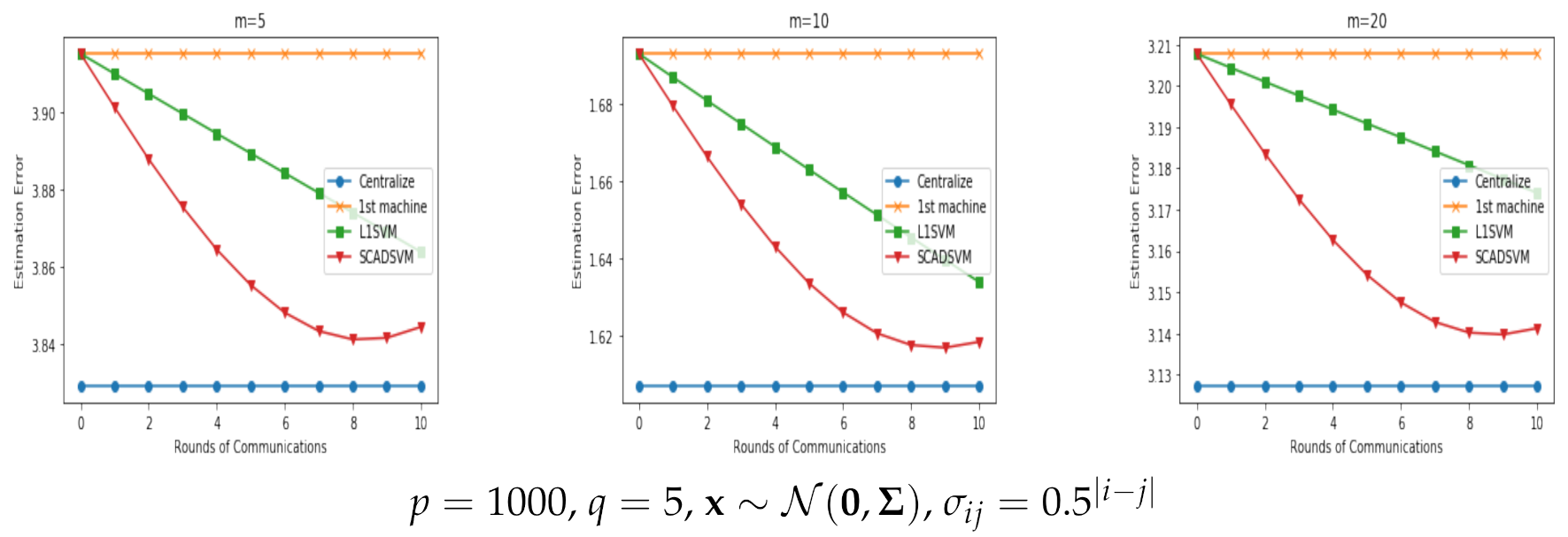
We use the first model to compare the performance of variable selection among the above four algorithms, which are listed in

Table 1. Variable selection results for Model 1.

		n = 200, p = 500
m	Sub	L1SVM	SCADSVM	Cen
5	21	2	1	0
10	22	3	4	0
15	28	0	1	0
20	24	0	0	0
		n = 200, p = 1000
m	Sub	L1SVM	SCADSVM	Cen
5	49	8	7	0
10	39	2	0	0
15	42	1	0	0
20	42	1	1	0
		n = 400, p = 500
m	Sub	L1SVM	SCADSVM	Cen
5	4	4	0	0
10	3	0	0	0
15	5	0	0	0
20	1	0	0	0
		n = 400, p = 1000
m	Sub	L1SVM	SCADSVM	Cen
5	6	0	0	0
10	7	0	0	0
15	4	0	0	0
20	4	0	0	0

; and use the other models to evaluate the estimation errors of parameters of algorithms via MSE, which are presented Figure 1, Figure 2 and Figure 3.

The numbers in Table 1 are the number of zero coefficients incorrectly estimated to be nonzero. The number of nonzero coefficients incorrectly estimated is zero, which meant all of the four algorithms could find the relevant variables; hence, they are not listed. From Table 1, we observed that:

(i)

The centralized algorithm was the best among these algorithms because it used the information of the whole dataset.

(ii)

The sub algorithm was bad because it only used the information of the data on the first machine.

(iii)

Our proposed L1SVM and SCADSVM could both select relevant variables, and the SCADSVM had a better performance than L1SVEM. This implied the non-convex SCADSVM algorithm was more robust than convex L1SVEM, especially for the complex models and massive datasets.

(iv)

When $N=mn$ was large, our two proposed distributed SVM algorithms were as good as the centralized algorithm.

We gave the prediction error analysis for models 2–4, see Figure 1, Figure 2 and Figure 3. From Figure 1, Figure 2 and Figure 3, we have the following observations:

(i)

The central algorithm was still the best classifier, but had the highest communication cost and risk of privacy leakage.There was a big gap between the sub estimator and the centralized estimator.

(ii)

Our two proposed communication-efficient estimators could match the central estimator with a few rounds of communication. The prediction errors of SCADSVM were lower than that of L1SVM, and it was more robust than L1SVM.

4.2. Real Data

In this subsection, we verify the performance of the CSLSVM algorithm (L1SVM and SCADSVM) using three real datasets. We use ‘a9a’, ‘w8a’, and ‘phishing’ datasets from the LIBSVM website (https://www.csie.ntu.edu.tw/∼cjlin/libsvm/ accessed on 12 February 2022). These real datasets are listed

Table 2. Real data used in the experiments.

Data Name	Number of Data	Features	Task
a9a	48,842	123	Classification
w8a	64,700	301	Classification
phishing	11,055	68	Classification

. The ‘a9a’ dataset was an adult dataset from the 1994 Census database. The prediction task was to determine whether a person makes over 50K a year or not. The ‘w8a’ dataset was also based on the Census database, but it had more features than ‘a9a’. The phishing dataset aimed to predict phishing websites. Phishing is the process by which a fraudster impersonates a legitimate person by simulating the same or similar web pages or websites to steal personal or private information for illegal political and economic gain. As phishing is becoming more and more serious, phishing web detection is gaining attention as an anti-phishing measure and technique.

Approximately 80% of the data was used to train the model and the remaining was applied to test the model. In distributed learning, we used the number of worker machines m = 5, 10, and 20, respectively. The results of classification errors for the three datasets are provided in Figure 4, Figure 5 and Figure 6. From Figure 4, Figure 5 and Figure 6, we found the following:

(i)

Since these datasets had no well-specified model, the curves behaved quite differently on these datasets. However, overall there was a large gap between the sub algorithm and centralized solution.

(ii)

In most of the cases, the distributed L1SVM algorithm still converged quite slowly.

(iii)

The proposed distributed SCADSVM could obtain a solution that was highly competitive with the centralized model within a few rounds of communications, and was more robust than the distributed L1SVM.

The experimental results on simulated and real datasets verified that the proposed distributed SCADSVM/L1SVM algorithms were two effective procedures for distributed sparse learning on classification via the SVM technique, which maintained efficiency in both communication and computation.

In the computational effort of the four methods, by numerical experiments, we also observed the following. For the central algorithm, the whole dataset was used to train the model, so it was the most accurate estimation, but had the highest computational cost and had a risk of privacy leakage. The sub-data estimation algorithm had the least computational cost because of the small amount of data, and no communication was required; however, it had the largest estimation error. Our proposed L1SVM and SCADSVM algorithms were communication efficient and computational efficient using the CSL framework, and could match the central estimator.

5. Conclusions

In the paper, we proposed a novel distributed CSLSVM learning algorithm with convex ($l_1$)/nonconvex (SCAD) penalties based on a communication-efficient surrogate likelihood (CSL) framework, which wads efficient in both communication and computation. For CSLSVM with $l_1$ penalty, we proved that the estimator of L1SVM could achieve a near-oracle property for an $l_1$ penalized SVM estimator based on the whole datasets. For CSLSVM with SCAD penalty, we showed that the estimator of SCADSVM enjoyed the oracle property, i.e., one of the local minimums of the distributed non-convex penalized SVM behaved similarly to the oracle estimator based on the whole dataset, as if the true sparsity was known in advance and only the relevant features were found to form the decision boundary. We also showed that, as long as the initial estimator was appropriate, the oracle estimator could be identified with a probability tending to 1. Extensive experiments on both simulated and real data illustrated that the proposed SCLSVM algorithm improved the performance of the work on the first worker machine and matched the centralized method. In addition, the proposed distributed SCADSVM could obtain a solution that was highly competitive with the centralized model within a few rounds of communication, and was more robust than the distributed L1SVM.

References

1. Vapnik, V. The Nature of Statistical Learning Theory; Springer Science & Business Media: Berlin/Heidelberg, Germany, 1995. [Google Scholar]
2. Banerjee, M.; Durot, C.; Sen, B. Divide and conquer in nonstandard problems and the super-efficiency phenomenon. Ann. Stat. 2019, 47, 720–757. [Google Scholar] [CrossRef] [Green Version]
3. Jordan, M.I.; Lee, J.D.; Yang, Y. Communication-Efficient Distributed Statistical Inference. J. Am. Stat. Assoc. 2019, 114, 668–681. [Google Scholar] [CrossRef] [Green Version]
4. Volgushev, S.; Chao, S.K.; Cheng, G. Distributed inference for quantile regression processes. arXiv 2017, arXiv:1701.06088. [Google Scholar] [CrossRef] [Green Version]
5. Chen, X.; Liu, W.; Mao, X.; Yang, Z. Distributed High-dimensional Regression Under a Quantile Loss Function. arXiv 2019, arXiv:1906.05741. [Google Scholar]
6. Wang, L.; Lian, H. Communication-efficient estimation of high-dimensional quantile regression. Anal. Appl. 2020, 18, 1057–1075. [Google Scholar] [CrossRef]
7. Zhang, Y.; Duchi, J.; Wainwright, M. Divide and conquer kernel ridge regression: A distributed algorithm with minimax optimal rates. J. Mach. Learn. Res. 2015, 16, 3299–3340. [Google Scholar]
8. Han, Y.; Mukherjee, P.; Ozgur, A.; Weissman, T. Distributed statistical estimation of high-dimensional and nonparametric distributions. In Proceedings of the 2018 IEEE International Symposium on Information Theory (ISIT), Vail, CO, USA, 17–22 June 2018; IEEE: Piscataway, NJ, USA, 2018; pp. 506–510. [Google Scholar]
9. Wang, X.; Yang, Z.; Chen, X.; Liu, W. Distributed inference for linear support vector machine. J. Mach. Learn. Res. 2019, 20, 1–41. [Google Scholar]
10. Zou, H. An improved 1-norm svm for simultaneous classification and variable selection. In Proceedings of the Eleventh International Conference on Artificial Intelligence and Statistics, PMLR, San Juan, Puerto Rico, 21–24 March 2007; pp. 675–681. [Google Scholar]
11. Meinshausen, N.; Bühlmann, P. High-dimensional graphs and variable selection with the lasso. Ann. Stat. 2006, 34, 1436–1462. [Google Scholar] [CrossRef] [Green Version]
12. Zhao, P.; Yu, B. On model selection consistency of Lasso. J. Mach. Learn. Res. 2006, 7, 2541–2563. [Google Scholar]
13. Meinshausen, N.; Yu, B. Lasso-type recovery of sparse representations for high-dimensional data. Ann. Stat. 2009, 37, 246–270. [Google Scholar] [CrossRef]
14. Zou, H. The adaptive lasso and its oracle properties. J. Am. Stat. Assoc. 2006, 101, 1418–1429. [Google Scholar] [CrossRef] [Green Version]
15. Bühlmann, P.; Van De Geer, S. Statistics for High-Dimensional Data: Methods, Theory and Applications; Springer Science & Business Media: Berlin/Heidelberg, Germany, 2011. [Google Scholar]
16. Giraud, C. Estimator Selection. In Introduction to High-Dimensional Statistics; Chapman and Hall: London, UK; CRC: London, UK, 2014; pp. 117–136. [Google Scholar]
17. Fan, J.; Fan, Y. High dimensional classification using features annealed independence rules. Ann. Stat. 2008, 36, 2605. [Google Scholar] [CrossRef] [Green Version]
18. Bradley, P.S.; Mangasarian, O.L. Feature selection via concave minimization and support vector machines. ICML Citeseer 1998, 98, 82–90. [Google Scholar]
19. Peng, B.; Wang, L.; Wu, Y. An error bound for l1-norm support vector machine coefficients in ultra-high dimension. J. Mach. Learn. Res. 2016, 17, 8279–8304. [Google Scholar]
20. Zhu, J.; Rosset, S.; Tibshirani, R.; Hastie, T.J. 1-norm support vector machines. Advances in neural information processing systems. Citeseer 2003, 16, 49–56. [Google Scholar]
21. Wegkamp, M.; Yuan, M. Support vector machines with a reject option. Bernoulli 2011, 17, 1368–1385. [Google Scholar] [CrossRef] [Green Version]
22. Fan, J.; Li, R. Variable selection via nonconcave penalized likelihood and its oracle properties. J. Am. Stat. Assoc. 2001, 96, 1348–1360. [Google Scholar] [CrossRef]
23. Becker, N.; Toedt, G.; Lichter, P.; Benner, A. Elastic SCAD as a novel penalization method for SVM classification tasks in high-dimensional data. BMC Bioinform. 2011, 12, 1–13. [Google Scholar] [CrossRef] [Green Version]
24. Park, C.; Kim, K.R.; Myung, R.; Koo, J.Y. Oracle properties of scad-penalized support vector machine. J. Stat. Plan. Inference 2012, 142, 2257–2270. [Google Scholar] [CrossRef]
25. Zhang, X.; Wu, Y.; Wang, L.; Li, R. Variable selection for support vector machines in moderately high dimensions. J. R. Stat. Soc. Ser. Stat. Methodol. 2016, 78, 53. [Google Scholar] [CrossRef] [Green Version]
26. Lian, H.; Fan, Z. Divide-and-conquer for debiased l1-norm support vector machine in ultra-high dimensions. J. Mach. Learn. Res. 2017, 18, 6691–6716. [Google Scholar]
27. Wang, J.; Kolar, M.; Srebro, N.; Zhang, T. Efficient Distributed Learning with Sparsity. arXiv 2016, arXiv:1605.07991. [Google Scholar]
28. Koo, J.Y.; Lee, Y.; Kim, Y.; Park, C. A bahadur representation of the linear support vector machine. J. Mach. Learn. Res. 2008, 9, 1343–1368. [Google Scholar]
29. Belloni, A.; Chernozhukov, V. l1-penalized quantile regression in high-dimensional sparse models. Ann. Stat. 2011, 39, 82–130. [Google Scholar] [CrossRef]
30. Van Der Vaart, A.W.; van der Vaart, A.W.; van der Vaart, A.; Wellner, J. Weak Convergence and Empirical Processes: With Applications to Statistics; Springer Science & Business Media: Berlin/Heidelberg, Germany, 1996. [Google Scholar]
31. Koltchinskii, V. Oracle Inequalities in Empirical Risk Minimization and Sparse Recovery Problems: Ecole d’Eté de Probabilités de Saint-Flour XXXVIII-2008; Springer Science & Business Media: Berlin/Heidelberg, Germany, 2011; Volume 2033. [Google Scholar]
32. Tao, P.; An, I. Convex analysis approach to D.C. programming theory, algorithms and applications. Acta Math. Vietnam. 1997, 22, 289–355. [Google Scholar]
33. Zou, H.; Li, R. One-step sparse estimates in nonconcave penalized likelihood models. Ann. Stat. 2008, 36, 1509. [Google Scholar]
Figure 1. Prediction error analysis vs. rounds of communication when m = 5 , 10, and 20 for model 2.
Mathematics 10 01029 g001
Figure 2. Prediction error analysis vs. rounds of communication when m = 5 , 10, and 20 for model 3.
Mathematics 10 01029 g002
Figure 3. Prediction error analysis vs. rounds of communication when m = 5 , 10, and 20 for model 4.
Mathematics 10 01029 g003
Figure 4. Classification error vs. rounds of communications for ’a9a’ data.
Mathematics 10 01029 g004
Figure 5. Classification error vs. rounds of communications for ’w8a’ data.
Mathematics 10 01029 g005
Figure 6. Classification error vs rounds of communications for ’phishing’ data.
Mathematics 10 01029 g006