CFD Analysis of Wind Distribution around Buildings in Low-Density Urban Community

Abstract

The computational fluid dynamics (CFDs) models based on the steady Reynolds-averaged Navier–Stokes equations (RANSs) using the $k-\omega$ two-equation turbulence model are considered in order to estimate the wind flow distribution around buildings. The present investigation developed a micro-scale city model with building details for the Hail area (Saudi Arabia) using ANSYS FLUENT software. Based on data from the region’s meteorological stations, the effect of wind speed (from 2 to 8 m/s) and wind direction (north, east, west, and south) was simulated. This study allows us to identify areas without wind comfort such as the corner of the building and the zones between adjacent buildings, which make this zone not recommended for placement of restaurants, pedestrian passages, or gardens. Particular attention was also paid to the highest building (Hail Tower, 67 m) in order to estimate, along the tower height, the wind speed effect on the turbulence intensity, the turbulent kinetic energy (TKE), the friction coefficient, and the dynamic pressure.

1. Introduction

Lower atmospheric wind studied around the buildings in urban areas [1] attracts the interest of many researchers due to the wide range of practical applications that could be treated. Such applications include urban wind energy production [2,3], air pollutants and dust dispersion [4,5], the effects of sandstorms on buildings [6], comfort and safety of pedestrians [7,8], etc.

Two approaches can tackle the study of urban wind. Firstly, the experimental approach [9,10], which is very costly and requires means to install several meteorological stations. Unfortunately, this approach can only give local measurements and is not well adapted to urban sites with a very diversified topography. With the improvement of computational tools and mesh generation software, the second numerical approach, using computational fluid dynamics (CFDs) [11,12,13,14,15], is becoming more and more interesting. In fact, CFDs, which are far less expensive in terms of time and money, provide local results in any point of the domain of study. Liu et al. [16] carried out a numerical study to simulate the distribution of the wind in urban areas. The mentioned authors built a full-scale model and construction details using the existing weather data of the community. This full-scale model is developed in the case of distance ranging from 2 to 20 km, which is positioned between “micro-scale” and “mesoscale” models. Three-dimensional RANS equations were resolved in order to find the urban wind flows. The performed model proved its capability to detect the wind topography in the community with an overestimation of the wind speed of 20% compared to the measured data on the roof building located on the site. Ricci et al. [17] investigated the accuracy and reliability of different turbulence models on steady three-dimensional RANS CFD simulations of wind flow for urban areas.

The influence of the k-ω as well as the k-ε turbulence models and roughness values are analyzed to measure their effect on the wind flow in complex urban areas. The authors performed a reduced-scale (1:300) model of a neighborhood in Livorno (Italy). The average wind velocity profile, turbulent kinetic energy (TKE), and turbulent dissipation obtained from measurements and CFD simulations were compared at several locations. They concluded that the turbulence model has a considerable effect on the distribution and topography of wind, while the surface roughness has no effect on the different flow parameters.

Kang et al. [18] studied the trees’ influence on enhancing wind comfort of pedestrians in urban areas. They exhaustively examined pedestrians’ wind comfort by considering the direction and the frequency of the wind. Special interest was also paid to the leaf surface density in order to reproduce the topography of the flow as closely as possible to the reality. The authors show that when the airflow passes through the trees, a clear wind comfort improvement for pedestrians was observed. The dispersion of pollutant emissions in an urban environment containing several buildings was studied by Chua et al. [19] for vehicle traffic and Toja-Silva et al. [20] for thermal power plant chimneys. The extent of pollution dispersion was determined for different wind speeds and directions. Feng and Gu [21] numerically studied the effect of wind veering on super high-rise buildings under different wind directions using large eddy simulations (LES). The authors concluded that the maximum wind loads occur in the range of 60°–75° of wind direction. Fan et al. [22] performed a numerical simulation on the blocking effect of buildings on airflow based on LES using the open FOAM code. The results showed that the spanwise width has an important effect on the horizontal recirculation flow.

Tominaga and Shirzadi [23] performed an experimental investigation using a wind tunnel on the flow structure around a group of buildings. The authors indicated the performed experiments can improve our understanding around the flow around actual buildings; a limitation was that they only used one wind direction. Zheng et al. [24] performed CFD simulations based on the k-ε turbulence model to predict the wind flow structure around a building with a focus on the effect of the surrounding buildings’ configurations. Liu et al. [9] used the LES technique to investigate the stratification effect on the wind over simplified tall buildings. The authors concluded that higher building density leads to less wind velocity fluctuations. Lee and Mak [25] studied the effects of wind direction and building arrangement on air flow structure and contaminant dispersion. It was found that the wind direction can be used to optimize the ventilation and pollutant dispersion. Kim et al. [26] used the deep learning and PIV technique to predict the flow around buildings. The combination of these two techniques represents a powerful tool, providing a better understanding of the flow structures around buildings.

Liu et al. [27] studied the flow around a building via the CFD with a focus on the effect of the surrounding buildings’ arrangement. The authors mentioned that their study is helpful in planning the urban configurations of buildings. Tamura et al. [28], experimenting with a wind tunnel, studied the effect of dimensions on the flow around a square building. Zheng et al. [29] experimentally studied the effect of aerodynamic on the wind load on tall buildings. The results showed that the building’s shape has an important effect on drag and lift forces. Zhou et al. [30] studied the effect of a twisted wind on the flow behavior around tall buildings. The authors used the LES for the computational analysis and a wind tunnel for the experiment investigation and showed that the twisted wind has a considerable effect on the flow structure around the building. Han et al. [31] performed a numerical study to validate the combined LBM-LES technique applied to a wind flow around a typical building. The authors mentioned that their method can provide very accurate results for the velocity field.

To the best of our knowledge, the computational fluid dynamics study of wind dispersion in a community with low density structures, and without vegetation (as in the case of most Gulf countries), has not been investigated. In this work, the effect of wind speed and direction in Hail City (Saudi Arabia) is analyzed and detailed.

2. Mathematical Formulation

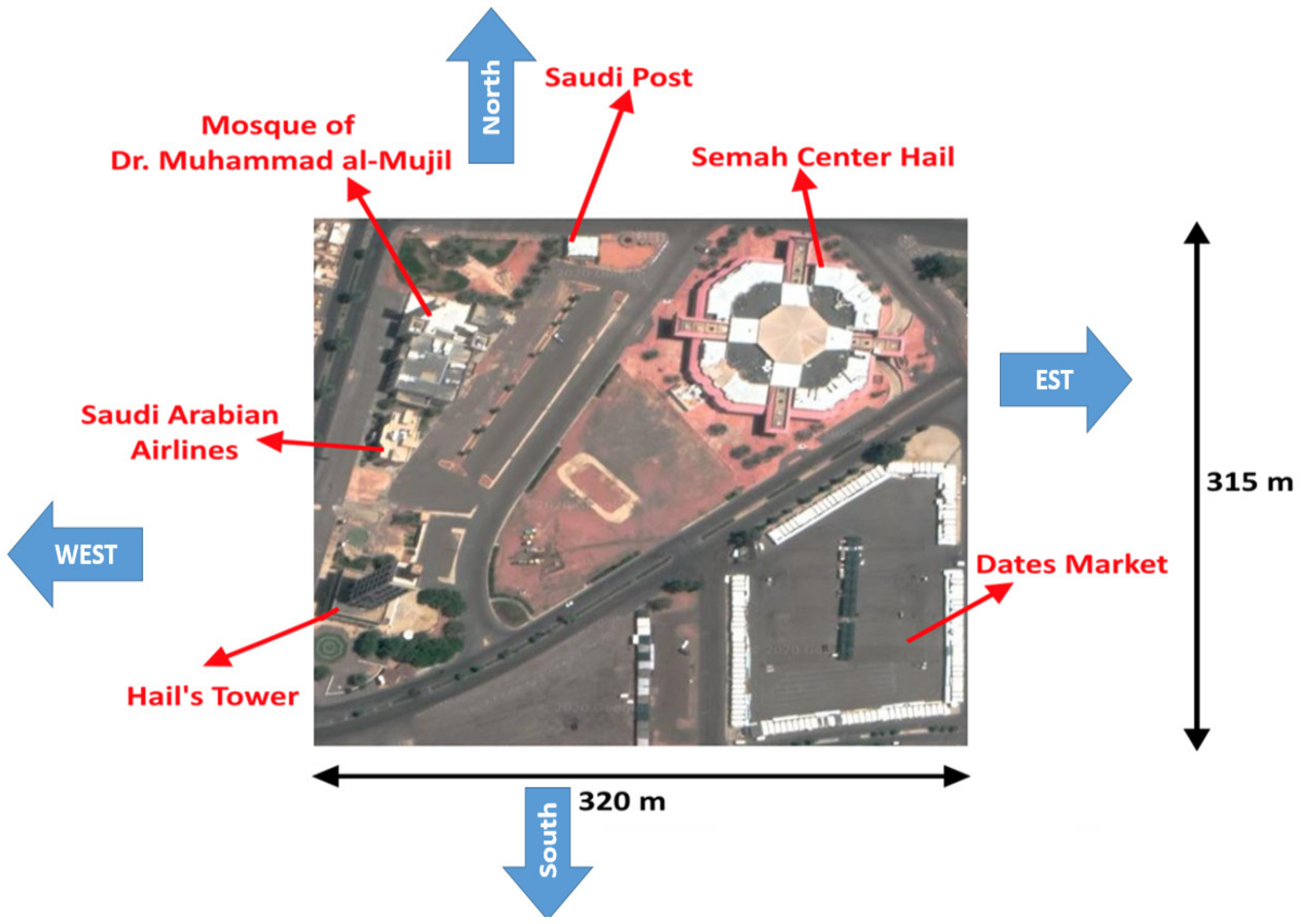
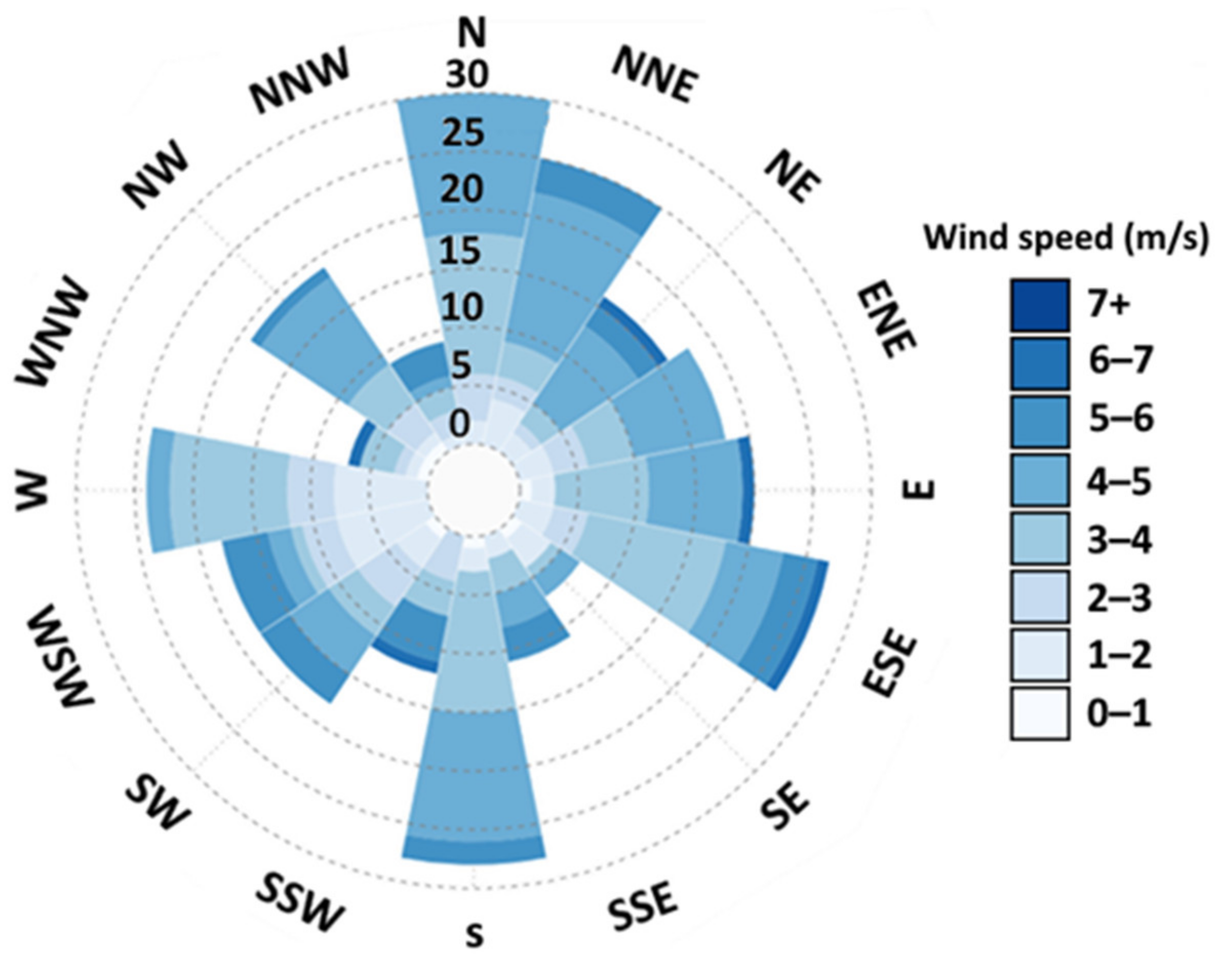
2.1. Real View of the Studied Area

A real view of the studied configuration is shown in Figure 1; this configuration is located at the city center at 27°31′23″ N and 41°41′50″ E and the buildings surrounding the study area are of low height. The site contains six compartments: Dates market, Semah Center Hail, Saudi Post, mosque of Dr. Muhammed al-Mujil, Saudi Arabian Airlines, and the Hail Tower. The ground is mainly composed of sand. Dimensions of the studied domain are 315 m along the axial direction (x-axis) and 320 m along the lateral (y-axis) direction, resulting in a total area of 100,800 m². The four orientations are presented in Figure 1.

2.2. Hypothesis

The considered RANS equations system is written with respect to the Cartesian coordinate with the origin o showed in Figure 2. The considered assumptions for the present investigation are as follows:

• Flow with three-dimensional (3D) aspect in steady state.
• Air is considered as the work fluid with constant physical and thermal properties.
• Flow with turbulent and fully developed aspect.
• Thermal effects due to the thermal gradient between the ground and the ambient air are neglected.

Figure 2. Geometric configuration and numerical domain.

Figure 2. Geometric configuration and numerical domain.

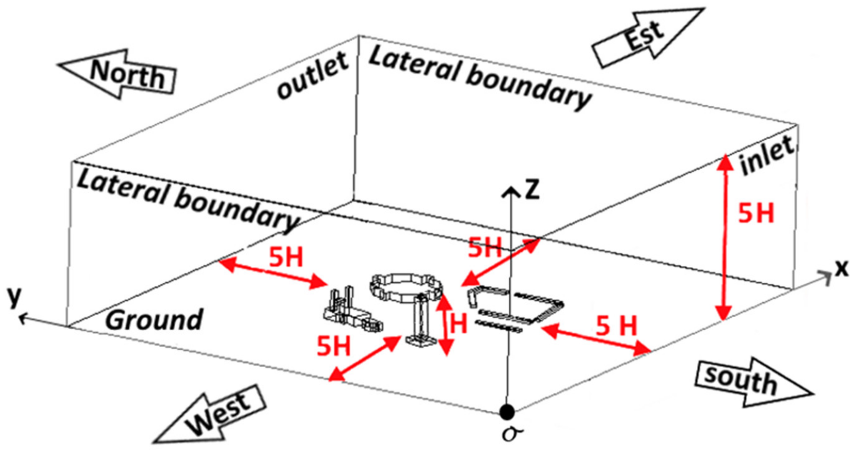
2.3. Geometric Configuration and Numerical Model

Figure 2 shows the numerical domain adapted for the present configuration. The tower height, H = 67 m, is considered as the reference value of all distances. The dimensions of the numerical domain are considered to be $\left(10H\times 10H\times 5H\right)$ along the x, y, and z-axis. The estimated blockage factor is therefore less than 0.3%. It seems important to note that all extensions of this domain have no effect on the present numerical results.

2.4. Governing Equations

The Reynolds-average Navier–Stocks (RANS) equations can be written in Cartesian tensor form as follows:

$$\frac{\partial }{\partial x_i}\left(\rho u_i\right)=0$$

(1)

$$\frac{\partial }{\partial x_j}\left(\rho u_i{u}_j\right)=-\frac{\partial p}{\partial x_i}+\frac{\partial }{\partial x_j}\left[\mu \left(\frac{\partial u_i}{\partial x_j}+\frac{\partial u_j}{\partial x_i}-\frac{2}{3}{\delta }_{ij}\frac{\partial u_l}{\partial x_l}\right)\right]+\frac{\partial }{\partial x_j}\left(-\rho \overline{u_i^{\prime }{u}_j^{\prime }}\right)$$

(2)

Additional terms now appear which represent the effect of turbulence. These Reynolds stresses must be modeled in order to close Equation (2). One common method employs the Boussinesq approximation to relate the Reynolds stress to the mean velocity gradient.

$$-\overline{\rho u_i^{\prime }{u}_j^{\prime }}={\mu }_t\left(\frac{\partial u_i}{\partial x_j}+\frac{\partial u_j}{\partial x_i}\right)-\frac{2}{3}\left(\rho k+{\mu }_t\frac{\partial u_k}{\partial x_k}\right){\delta }_{ij}$$

(3)

The turbulent kinetic energy k and its specific dissipation rate ω are obtained from the following equations:

$$\frac{\partial }{\partial x_i}\left(\rho k{u}_i\right)=\frac{\partial }{\partial x_j}\left({\mathrm{\Gamma }}_k\frac{\partial k}{\partial x_j}\right)+G_k-Y_k+S_k$$

(4)

$$\frac{\partial }{\partial x_i}\left(\rho \omega u_i\right)=\frac{\partial }{\partial x_j}\left({\mathrm{\Gamma }}_w\frac{\partial \omega }{\partial x_j}\right)+G_{\omega }-Y_{\omega }+S_{\omega }$$

(5)

In these equations, G_k and G${}_{\omega }$ represent, respectively, the generation of k and ω due to the mean velocity gradient. ${\mathrm{\Gamma }}_k$ and ${\mathrm{\Gamma }}_{\omega }$ are, respectively, the effective diffusivity for k and ω. Y_k and Y${}_{\omega }$ are the dissipation of k and ω, respectively, due to the turbulence. S_k and S${}_{\omega }$ are the source terms for turbulent kinetic energy and its source dissipation ratio (considered to be zero in the present simulation), respectively. The default value of the turbulent Prandtl number Pr_t is 0.85. The effective diffusivity for the k-ω model is given by the following expression:

$${\mathrm{\Gamma }}_k=\mu +\frac{{\mu }_t}{{\sigma }_k}$$

(6)

$${\mu }_t={\alpha }^{*}\frac{\rho k}{\omega }$$

(7)

$${\mathrm{\Gamma }}_{\omega }=\mu +\frac{{\mu }_{\omega }}{{\sigma }_{\omega }}$$

(8)

where ${\sigma }_k$ and ${\sigma }_{\omega }$ are the turbulent Prandtl numbers, respectively, for k and ω.

$${\alpha }^{*}={\alpha }_{\infty }^{*}\left(\frac{{\alpha }_0^{*}+\raisebox{1ex}{${Re}_t$}\!\left/ \!\raisebox{-1ex}{$R_k$}\right.}{1+\raisebox{1ex}{${Re}_t$}\!\left/ \!\raisebox{-1ex}{$R_k$}\right.}\right)$$

(9)

$${Re}_t=\frac{\rho k}{\mu \omega }$$

(10)

$${\alpha }_0^{*}=\frac{{\beta }_i}{3}$$

(11)

$R_k$ and ${\beta }_i$ constant value (

Table 1. Values of the constant used in Equations (1)–(29).

${\mathit{\alpha }}_{\mathit{\infty }}^{*}$	${\mathit{\alpha }}_{\mathit{\infty }}$	${\mathit{\alpha }}_{\mathbf{0}}$	${\mathit{\beta }}_{\mathit{\infty }}^{*}$	${\mathit{\beta }}_{\mathit{i}}$	${\mathit{R}}_{\mathit{\beta }}$	${\mathit{R}}_{\mathit{k}}$	${\mathit{R}}_{\mathit{w}}$	${\mathit{\zeta }}^{*}$	${\mathit{M}}_{\mathit{t}\mathbf{0}}$	${\mathit{\sigma }}_{\mathit{k}}$	${\mathit{\sigma }}_{\mathit{w}}$
1	0.52	1/9	0.09	0.072	8	6	2.95	1.5	0.25	2	2

). It is noted that for the k-ω model with a high Reynolds number, ${\alpha }^{*}={\alpha }_{\infty }^{*}=1$. The production of turbulent kinetic energy $G_k$ and the production of its specific dissipation $G_w$ in Equations (4) and (5), respectively, are defined by:

$$G_k=-\rho \overline{u_i^{\prime }{u}_j^{\prime }}\frac{\partial u_j}{\partial x_i}$$

(12)

$$G_k={\mu }_t{S}^2$$

(13)

$$S\equiv \sqrt{2S_{ij}{S}_{ij}}$$

(14)

$$G_w=\alpha \frac{w}{k}{G}_k$$

(15)

$$\alpha =\frac{{\alpha }_{\infty }}{{\alpha }^{*}}\left(\frac{{\alpha }_0+\raisebox{1ex}{${Re}_t$}\!\left/ \!\raisebox{-1ex}{$R_w$}\right.}{1+\raisebox{1ex}{${Re}_t$}\!\left/ \!\raisebox{-1ex}{$R_w$}\right.}\right)$$

(16)

where $R_{\omega }$ is constant value (Table 1), ${Re}_t$ and ${\alpha }^{*}$ are given by Equations (10) and (11), respectively. It is noted that for the k-ω model with a high Reynolds number, $\alpha ={\alpha }^{*}=1$. The dissipation of the turbulent kinetic energy $Y_k$ is given by:

$$Y_k=\rho {\beta }^{*}{f}_{{\beta }^{*}}k\omega$$

(17)

$$\begin{gathered} f_{{\beta }^{*}}=1 \mathrm{if} {\chi }_k\le 0 \\ {f}_{{\beta }^{*}}=\frac{1+680{\chi }_k{}^2}{1+400{\chi }_k{}^2} \mathrm{if} {\chi }_k\le 0 \end{gathered}$$

(18)

$${\chi }_k\equiv \frac{1}{{\omega }^3}\frac{\partial k}{\partial x_j}\frac{\partial \omega }{\partial x_j}$$

(19)

$${\beta }^{*}={\beta }_i^{*}\left[1+{\zeta }^{*}F(M_t)\right]$$

(20)

$${\beta }_i^{*}={\beta }_{\infty }^{*}\left(\frac{\raisebox{1ex}{$4$}\!\left/ \!\raisebox{-1ex}{$15$}\right.+{\left(\raisebox{1ex}{${Re}_t$}\!\left/ \!\raisebox{-1ex}{$R_{\beta }$}\right.\right)}^4}{1+{\left(\raisebox{1ex}{${Re}_t$}\!\left/ \!\raisebox{-1ex}{$R_{\beta }$}\right.\right)}^4}\right)$$

(21)

where ${\zeta }^{*}$, $R_{\beta }$, and ${\beta }_{\infty }^{*}$ are constant values (Table 1) and ${Re}_t$ is given by Equation (10). The dissipation of ω is given as follows:

$$Y_w=\rho \beta f_{\beta }{\omega }^2$$

(22)

$$f_{\beta }=\frac{1+70{\chi }_w}{1+80{\chi }_w}$$

(23)

$${\chi }_w=\left|\frac{{\mathsf{\Omega }}_{ij}{\mathsf{\Omega }}_{jk}{\mathsf{\Omega }}_{ki}}{{\left({\beta }_{\infty }^{*}\omega \right)}^3}\right|$$

(24)

$${\mathsf{\Omega }}_{ij}=\frac{1}{2}\left(\frac{\partial u_i}{\partial x_j}-\frac{\partial u_j}{\partial x_i}\right)$$

(25)

$$\beta ={\beta }_i\left[1-\frac{{\beta }_i^{*}}{{\beta }_i}{\zeta }^{*}F(M_t)\right]$$

(26)

$$\begin{gathered} F\left(M_t\right)=1 \mathrm{if} M_t\le M_{t0} \\ F\left(M_t\right)=M_t^2-M_{t0}^2 \mathrm{if} M_t\succ M_{t0} \end{gathered}$$

(27)

$$M_t^2=\frac{2k}{a^2}$$

(28)

$$a=\sqrt{\gamma RT}$$

(29)

For the k-ω turbulence model with a high Reynolds number, ${\beta }_i^{*}={\beta }_{\infty }^{*}$, and for incompressible flow, ${\beta }^{*}={\beta }_i^{*}$. Table 1 summarizes the different constants cited above.

The drag force energy and its specific dissipation rate are obtained from the following equations:

$$F_D=\frac{1}{2}{C}_D\rho V^{2}A$$

(30)

where C_D is the drag coefficient

$$C_D=C_f+C_P$$

(31)

C_f is the friction drag coefficients and C_p is the pressure drag coefficients.

It should be noted that, although the climate of the region under study is particularly warm and the thermophysical properties can vary with temperature, movements due to the natural convection can take place. We tried some simulations using the Boussinesq approximation ($\rho ={\rho }_0+\beta \left(T-T_0\right)$) without noticing any variation in the results. In fact, given the wind speed used in this work of 4 m/s, the inertial forces are predominant and all other thermal forces, such as thermal buoyancy forces, can be neglected.

2.5. Grid Distribution and Boundary Conditions

Refined tetrahedral mesh is adopted in the vicinity of the compartment surfaces and more relaxed mesh elsewhere. Grid is uniformly adopted in all of the compartment segment (Figure 3) with a mesh spacing s = 3. For the numerical domain segment, uniform mesh is used with a spacing s = 15. The volume mesh evolved from the compartment’s surfaces until the domain external surface reached an expansion ratio e = 1.2, giving a final number of cells in all the domains equal to 800 × 103. In the present simulation, the standard k-ω turbulence model, with the enhanced wall treatment employed to resolve the laminar sublayer, y+ at the wall-adjacent cell should be on the order of y+ = 1. However, a higher y+ is acceptable as long as it is well inside the viscous sublayer (y+ < 4 to 5). The present mesh near the wall is fine enough to assure these limit values of y+.

At the inlet, the VELOCITY INLET boundary condition is considered, and the velocity profile (boundary layer profile) at the inlet is chosen to ensure the development of the atmospheric boundary layer. At the “Ground + Building”, the WALL boundary with no slip condition is adopted (u = 0, v = 0, and w = 0). Note that u, v, and w present, respectively, the velocity component along the x, y, and z axis. We also apply the “lateral boundary” PRESSURE INLET condition and, finally, the “outlet” PRESSURE OUTLET boundary condition (Figure 3). At these boundaries (PRESSURE INLET and PRESSURE OUTLET), the pressure is equal to the atmospheric pressure (P = P_a) and $\frac{\partial u}{\partial y}=\frac{\partial v}{\partial y}=\frac{\partial k}{\partial y}=\frac{\partial \omega }{\partial y}=0$.

At the inlet boundary, the turbulent kinetic energy k and its specific dissipation rate ω are given by the following expression:

$$k_0=\frac{3}{2}{\left(I{u}_0\right)}^2$$

(32)

$${\omega }_0=\frac{k_0^{1/2}}{C_{\mu }^{1/4}0.07d}$$

(33)

where I is the turbulence intensity taken from the meteorological condition of Hail City I = 5%, u₀ is the average value of the inlet velocity (in the present study u₀ = 2, 4, 6, and 8 m/s), C_μ is a constant value equal to 0.09, and d is the hydraulic diameter d = 457 m. Based on the different considered inlet velocity, we obtained the following values of k₀ and ω₀. The imposed values of k₀ and ω₀ imposed at the inlet boundary are presented in

Table 2. k₀ and ω₀ values at the inlet boundary.

u0 (m/s)	k0 (m²/s)	ω0 (1/s)
2	0.015	0.007
4	0.06	0.014
6	0.135	0.021
8	0.24	0.028

.

2.6. Numerical Method

The governing equations are numerically solved using ANSYS FLUENT software based on the finite volume method developed by Pantakar [32]. The method of numerical resolution consists of integrating the momentum conservation, the mass conservation, the (TKE) turbulence kinetic energy k, as well as the specific dissipation rate of the turbulent kinetic energy ω equations on each control volume. The discretization of these equations is based on the second-order upwind technique. More detail on this technique can be found in Ref. [33]. The velocity–pressure coupling is based on the “SIMPLEC” algorithm. The considered convergence criterion is 10⁻⁴. We have verified that decreasing this convergence criterion has practically no effect on the results.

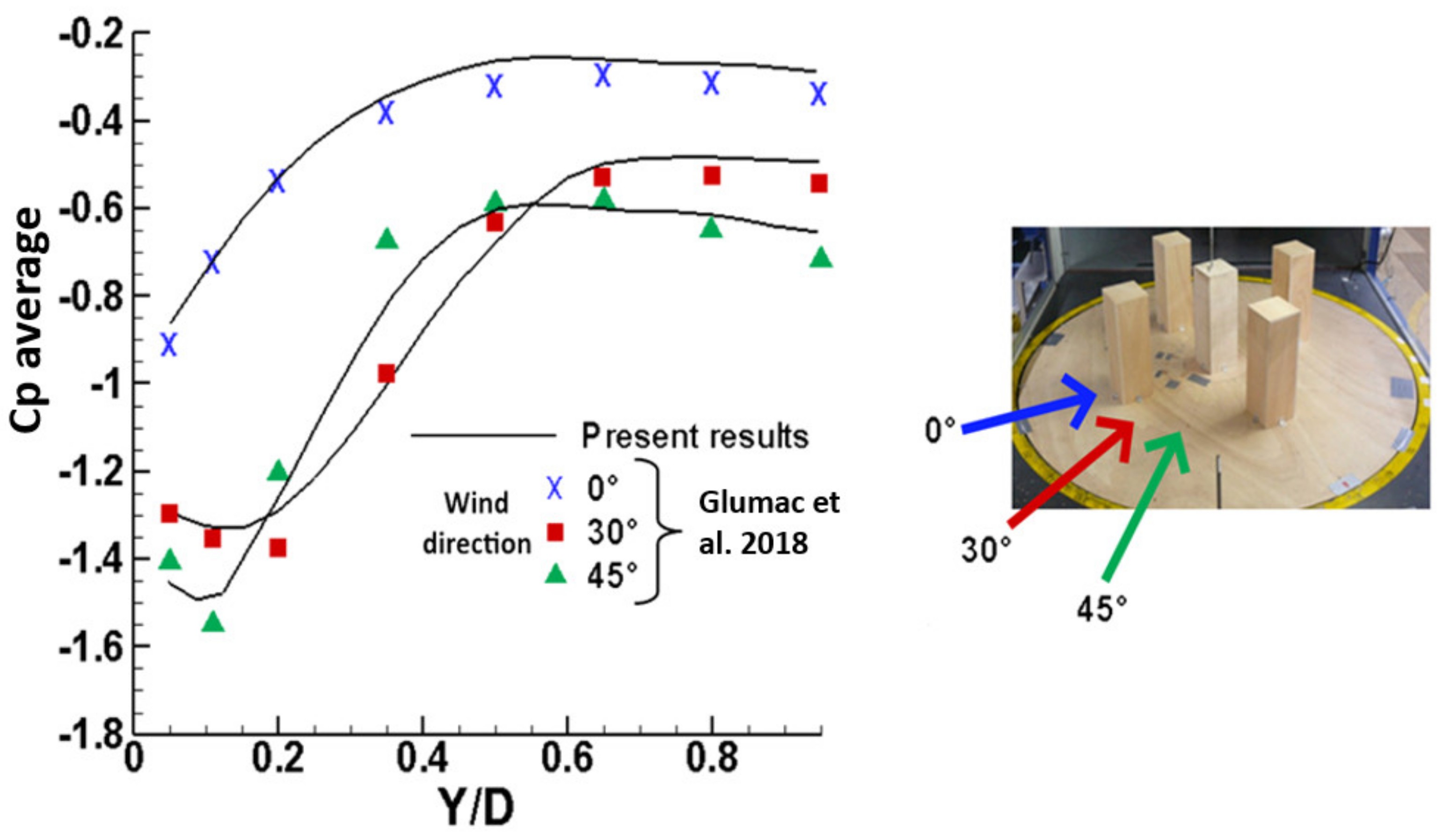
2.7. Validation Test

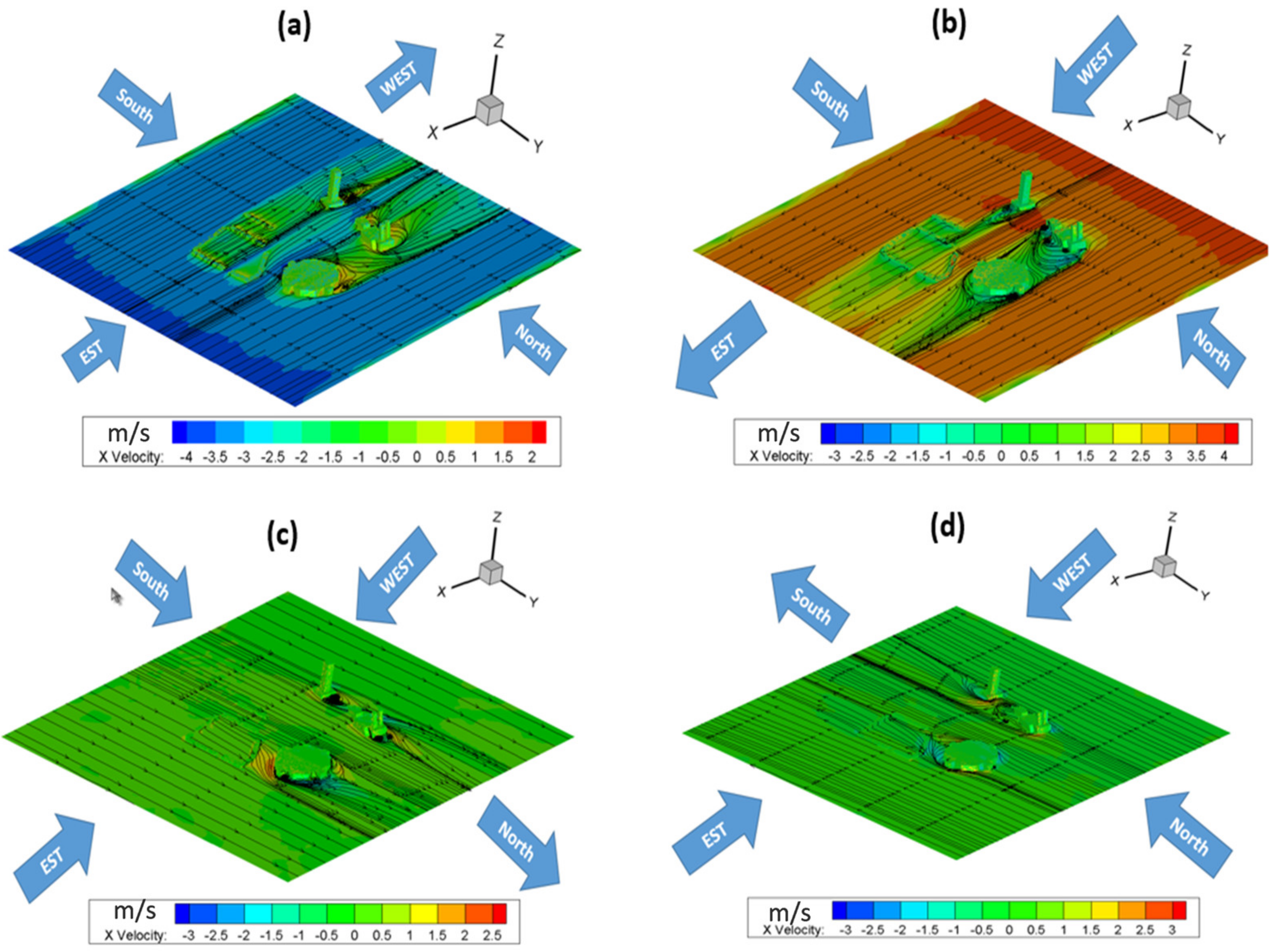
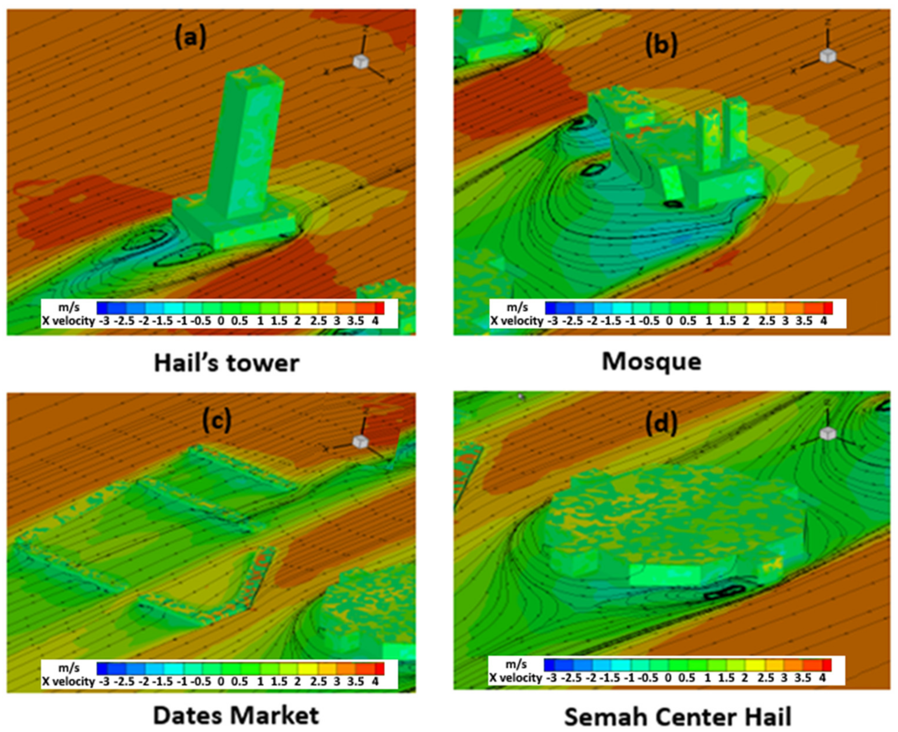
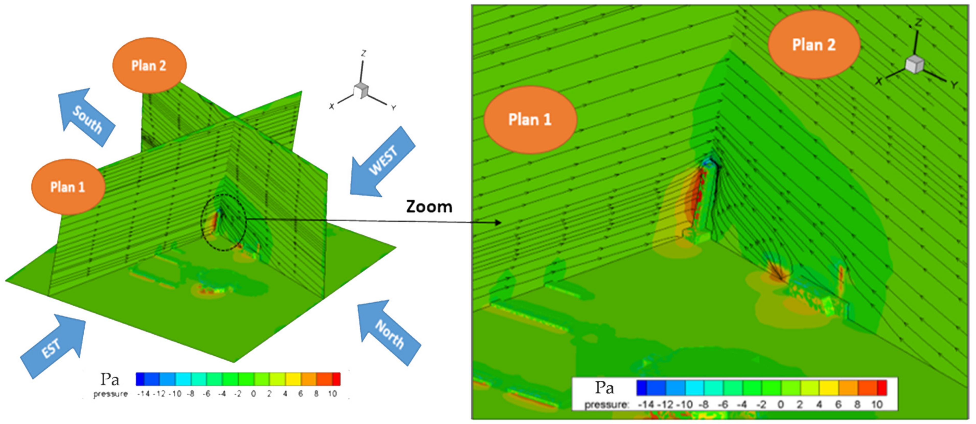
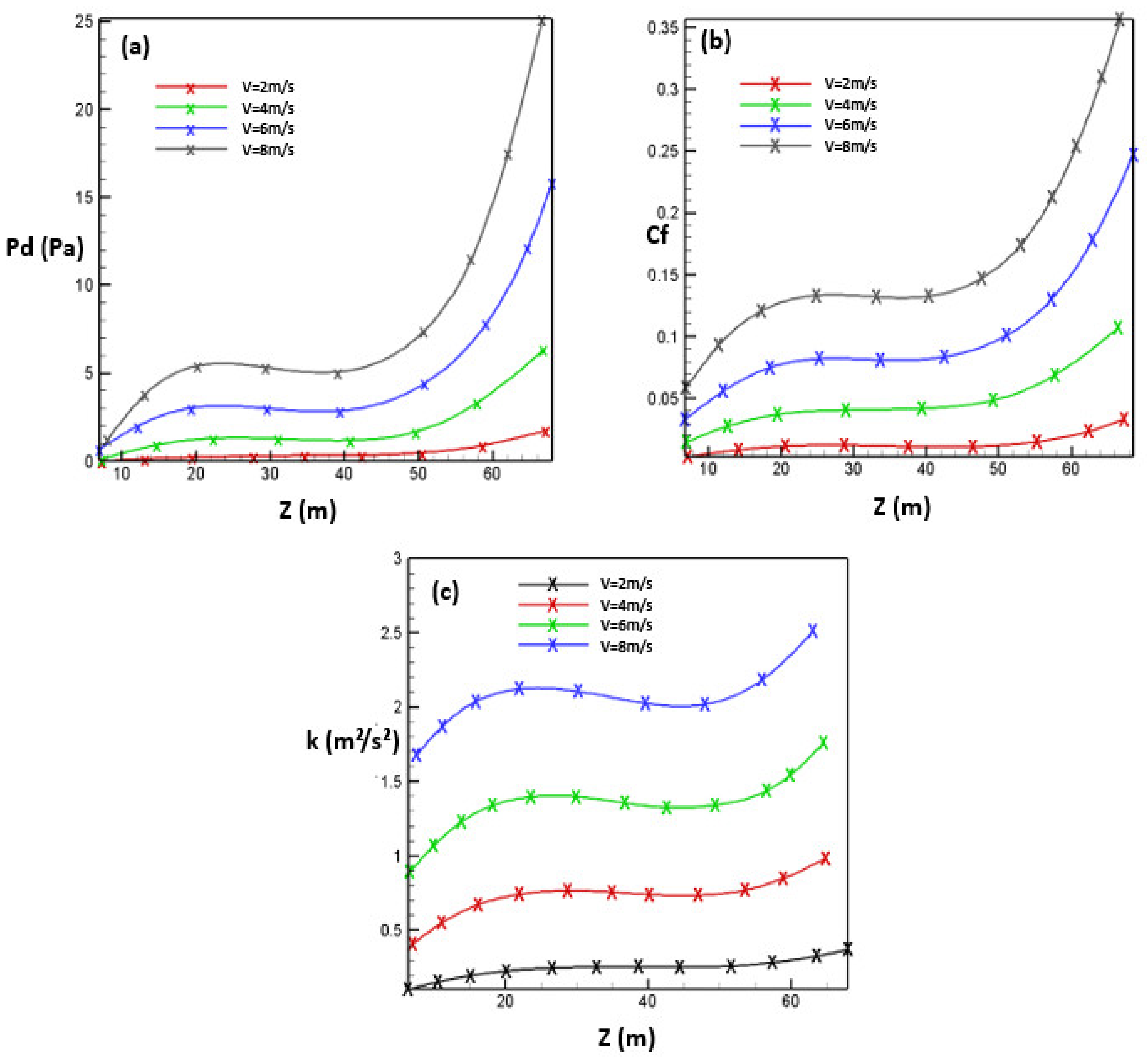
In order to validate our numerical model, we performed simulations under the numerical conditions of Ramponi et al. [13]. This numerical work was carried out on an urban configuration composed of regular arrays of rectangular buildings with a plan area of 16 × 24 m² and heights of 18 m. Two plots are validated in the present section: the axial velocity U (Figure 4a) and the pressure coefficient C_p (Figure 4b). As shown in Figure 4, our chosen model uses the simple algorithm (semi-implicit method for pressure-linked equations) with the k-ω turbulence model and for three different mesh sizes, i.e., 128 × 10³ cells, 400 × 10³ cells, and 600 × 10³ cells. Figure 4a clearly shows a noticeable difference between the plot using 128 × 10³ and 400 × 10³ cells, whereas no significant difference is observed between plots with 400 × 10³ and 600 × 10³ cells. So, the grid-size convergence is reached for the 400 × 10³ cells, which allows reduced calculation times and delivers results in agreement with Ramponi et al. [13], with an error rate of less than 2.5%.

In Figure 4b, we show the pressure coefficient plot for different turbulence models, such as the standard k-ω, SST k-ω, the standard k-ε, as well as the RSM model. It can be construed from Figure 4b that the k-ω turbulence model shows the best agreement with the results of Ramponi et al. [13] compared to other turbulence models.

In Figure 5, further validation tests with the experimental work of Glumac et al. [10] were conducted. These tests were carried out with a wind tunnel using a prototype composed of five high buildings. The pressure coefficient profiles show good agreement in comparison with the experimental measurements, with a maximum error rate of about 8.2%.

3. Results

According to our weather station located at the University of Hail at about 10 m above ground level (Figure 6), the average wind speed throughout the year is estimated to be between 3.5 (September) and 4.4 m/s (March), i.e., an annual average of 4 m/s. The wind rose plotted for the years 2020/2021 (Figure 7) shows that there are no real preferential directions.

In Figure 8, we present the streamlines in addition to the axial velocity contours (along the x-axis) for 4 m/s wind speed coming from different directions: EAST (a), WEST (b), SOUTH (c), and NORTH (d). A zoomed view of the vicinity of the various buildings is presented in Figure 9 to clearly show the vortices formation, as well as the high-velocity zones.

It can be observed from Figure 8 that the streamlines are serried around buildings while they are looser and aligned away from buildings. This is due to the friction of the wind against the surfaces of buildings. The contours of the axial velocity also show red color zones, which indicate an acceleration of the velocity along the corners of the buildings. These regions of high velocity are not very comfortable for pedestrians, and it is not recommended to place restaurants, pedestrian passages, or gardens nearby.

Figure 9 clearly shows that on these corners, the wind tries to escape when it is confronted with building surfaces, which causes a sudden velocity acceleration. The same figure also shows the formation of recirculation vortices in the upstream part of the flow. The zones where vortices are formed are characterized by a reversed flow (negative value of the axial speed) and by a depression (negative value of the pressure).

Behind the Hail Tower, two vortices are formed downstream of the flow; these counter-rotated vortices are identical in the case of symmetrical geometry (Figure 9a). Vortices are also formed at the building’s corners and the velocity acceleration is clear (Figure 9b–d).

On the other hand, a phenomenon called the Venturi effect can also be seen in Figure 9a,b. This phenomenon happens when the flow crosses between the mosque and the Hail Tower (Figure 9b). In this region, we can observe that the streamlines are more compact when the flow passes. Along the latter mentioned zone, an increase in the velocity and a decrease in the pressure (depression zone) constitute negative conditions for pedestrian comfort.

In order to show the flow evolution around the height of the Hail Tower, Figure 10 presents the streamlines in addition to the axial velocity contours around the Hail Tower passing by plans 1 and 2. As clearly shown in Figure 10, in the vicinity of the Hail Tower, the streamline serried due to the shearing effect of the flow on the building surfaces. Red color zones highlight the acceleration of the flow when trying to cross the building surfaces. Open windows in these levels will generate disturbances and violent draughts for the occupants.

To study the characteristics of the flow in the vicinity of the Hail Tower for SOUTH direction wind with different velocities V = 2, 4, 6, and 8 m/s, we show the evolution of dynamic pressure P_d (Figure 11a), the friction coefficient C_f (Figure 11b), and the turbulent kinetic energy k (Figure 11c).

It can be observed that the dynamic pressure, the friction coefficient, and the turbulent kinetic energy, respectively, continue to increase up to the height of 30 m. This clearly shows the increase in the turbulence level on the vicinity of the tower’s surfaces. From a height z = 30 m up to z = 40 m, all the curves have a plateau region; this is expressed by constant values of the dynamic pressure, the friction coefficient, and the turbulent kinetic energy. This clearly shows stabilization in the level of turbulence in the vicinity of the Hail Tower for a height along this intermediate zone. From z = 40 m, the curves continue to increase up to a height z = 67 m.

We can observe that, for the different curves along the first zone (up to z = 30 m), the rate of the dynamic pressure, friction coefficient, and turbulent kinetic energy all increase with the wind velocity. This shows that the intensification of the turbulence level while ascending in height is more pronounced for large values of wind velocity. Along the second zone, between z = 30 and z = 40 m, P_d, C_f, and k remain constant when varying z and increasing amplitude for large values of the wind velocity. Along the third zone (z = 40 up to z = 67 m), the growth rate of the different curves is strongly influenced by the wind speed. We can clearly observe that the slope of the P_d, C_f, and k as a function of z increases with wind velocity, which shows the intensification of the height effect on the turbulence level as the wind speed increases. Thus, the top of the tower has a high turbulence zone when the air speed exceeds 4 m/s. It is therefore strongly discouraged to install a landing zone for helicopters, for example, or to plan any human activity in the open air.

4. Conclusions

A numerical investigation was conducted to study the wind distribution around buildings in a low-density urban community using ANSYS FLUENT software. The city center of Hail in Saudi Arabia was used as the study area. Several wind directions and speeds were considered. In this study, we were able to identify areas of wind discomfort, specifically areas characterized by high depression and high turbulence. Special attention was given to the Hail Tower (the tallest building in the region). We were able to identify and locate the various vortices that arise in the wake of the tower. It was also shown, through the estimation of the dynamic pressure, the friction coefficient, and the turbulent kinetic energy, that from an altitude of 30 m, the level of turbulence near the tower’s surfaces increases considerably. Depending on the wind speed, an intensification of up to 730% of the turbulent kinetic energy was noted for a variation of 2 to 8 m/s. Finally, this work studies the wind comfort of pedestrians in urban areas and confirms that weather conditions (wind speed and direction) and building layout are key parameters for comfort.

References

1. Blocken, B.; Stathopoulos, T.; Carmeliet, J. CFD simulation of the atmospheric boundary layer: Wall function problems. Atmos. Environ. 2007, 41, 238–252. [Google Scholar] [CrossRef]
2. Rezaeiha, A.; Montazeri, H.; Blocken, B. A framework for preliminary large-scale urban wind energy potential assessment: Roof-mounted wind turbines. Energy Convers. Manag. 2020, 214, 112770. [Google Scholar] [CrossRef]
3. Zinat, T.; Al Noman, A.; Sajal, K. An analytical review on the evaluation of wind resource and wind turbine for urban application: Prospect and challenges. Dev. Built Environ. 2020, 4, 100033. [Google Scholar] [CrossRef]
4. Keshavarzian, E.; Jin, R.; Dong, K.; Kwok, K.C.; Zhang, Y.; Zhao, M. Effect of pollutant source location on air pollutant dispersion around a high-rise building. Appl. Math. Model. 2020, 81, 582–602. [Google Scholar] [CrossRef] [PubMed]
5. Tiwari, A.; Prashant, K. Integrated dispersion-deposition modelling for air pollutant reduction via green infrastructure at an urban scale. Sci. Total Environ. 2020, 723, 138078. [Google Scholar] [CrossRef] [PubMed]
6. Sarafrazi, V.; Talaee, M.R. Simulation of wall barrier properties along a railway track during a sandstorm. Aeolian Res. 2020, 46, 100626. [Google Scholar] [CrossRef]
7. Razak, A.A.; Hagishima, A.; Salim, S.A.Z.S. Progress in wind environment and outdoor air ventilation at pedestrian level in urban area. Appl. Mech. Mater. 2016, 819, 236–240. [Google Scholar] [CrossRef]
8. Blocken, B.; Janssen, W.D.; van Hooff, T. CFD simulation for pedestrian wind comfort and wind safety in urban areas: General decision framework and case study for the Eindhoven University campus. Environ. Model. Softw. 2012, 30, 15–34. [Google Scholar] [CrossRef]
9. Liu, Z.; Li, W.; Shen, L.; Han, Y.; Zhu, Z.; Hua, X. Numerical study of stable stratification effects on the wind over simplified tall building models using large-eddy simulations. Build. Environ. 2021, 193, 107625. [Google Scholar] [CrossRef]
10. Glumac, A.Š.; Hemida, H.; Höffer, R. Wind energy potential above a high-rise building influenced by neighboring buildings: An experimental investigation. J. Wind Eng. Ind. Aerodyn. 2018, 175, 32–42. [Google Scholar] [CrossRef] [Green Version]
11. Jin, M.; Zuo, W.; Chen, Q. Simulating natural ventilation in and around buildings by fast fluid dynamics. Numer. Heat Transf. Part A Appl. 2013, 64, 27–289. [Google Scholar] [CrossRef]
12. Chen, Q.; Glicksman, L.R.; Lin, J. Chapter 7: Design of natural ventilation with CFD. In Sustainable Urban. Housing in China; Springer: Berlin/Heidelberg, Germany, 2006; pp. 116–123. [Google Scholar] [CrossRef]
13. Ramponi, R.; Blocken, B.; De Coo, L.B.; Janssen, W.D. CFD simulation of outdoor ventilation of generic urban configurations with different urban densities and equal and unequal street widths. Build. Environ. 2015, 92, 152–166. [Google Scholar] [CrossRef] [Green Version]
14. Sheremet, M.A.; Miroshnichenko, I.V. Numerical study of turbulent natural convection in a cube having finite thickness heat-conducting walls. Heat Mass Transf. 2015, 51, 1559–1569. [Google Scholar] [CrossRef]
15. Miroshnichenko, I.V.; Sheremet, M.A. Turbulent natural convection heat transfer in rectangular enclosures using experimental and numerical approaches: A review. Renew. Sustain. Energy Rev. 2018, 82, 40–59. [Google Scholar] [CrossRef]
16. Liu, S.; Pan, W.; Zhang, H.; Cheng, X.; Long, Z.; Chen, Q. CFD simulations of wind distribution in an urban community with a full-scale geometrical model. Build. Environ. 2017, 117, 11–23. [Google Scholar] [CrossRef]
17. Ricci, A.; Kalkman, I.; Blocken, B.; Burlando, M.; Repetto, M.P. Impact of turbulence models and roughness height in 3D steady RANS simulations of wind flow in an urban environment. Build. Environ. 2020, 171, 106617. [Google Scholar] [CrossRef]
18. Kang, G.; Kim, J.J.; Choi, W. Computational fluid dynamics simulation of tree effects on pedestrian wind comfort in an urban area. Sustain. Cities Soc. 2020, 56, 102086. [Google Scholar] [CrossRef]
19. Chu, A.K.M.; Kwok, R.C.W.; Yu, K.N. Study of pollution dispersion in urban areas using Computational Fluid Dynamics (CFD) and Geographic Information System (GIS). Environ. Model. Softw. 2005, 20, 273–277. [Google Scholar] [CrossRef]
20. Toja-Silva, F.; Pregel-Hoderlein, C.; Chen, J. On the urban geometry generalization for CFD simulation of gas dispersion from chimneys: Comparison with Gaussian plume model. J. Wind Eng. Ind. Aerodyn. 2018, 177, 1–18. [Google Scholar] [CrossRef]
21. Feng, C.; Gu, M. Numerical simulation of wind veering effects on square-section super high-rise buildings under various wind directions. J. Build. Eng. 2021, 44, 102954. [Google Scholar] [CrossRef]
22. Fan, M.; Li, W.J. Parameterised drag model for the underlying surface roughness of buildings in urban wind environment simulation. Build. Environ. 2022, 209, 108651. [Google Scholar] [CrossRef]
23. Tominaga, Y.; Shirzadi, M. Wind tunnel measurement of three-dimensional turbulent flow structures around a building group: Impact of high-rise buildings on pedestrian wind environment. Build. Environ. 2021, 206, 108389. [Google Scholar] [CrossRef]
24. Zheng, S.; Wang, Y.; Zhai, Z.; Xue, Y.; Duanmu, L. Characteristics of wind flow around a target building with different surrounding building layers predicted by CFD simulation. Build. Environ. 2021, 201, 107962. [Google Scholar] [CrossRef]
25. Lee, K.Y.; Mak, C.M. Effects of wind direction and building array arrangement on airflow and contaminant distributions in the central space of buildings. Build. Environ. 2021, 205, 108234. [Google Scholar] [CrossRef]
26. Kim, B.; Lee, D.E.; Preethaa, K.R.S.; Hu, G.; Natarajan, Y.; Kwok, K.C.S. Predicting wind flow around buildings using deep learning. J. Wind Eng. Ind. Aerodyn. 2021, 219, 104820. [Google Scholar] [CrossRef]
27. Sumei, L.; Pana, W.; Zhaoa, X. Influence of surrounding buildings on wind flow around a building predicted by CFD simulations. Build. Environ. 2018, 140, 1–10. [Google Scholar] [CrossRef]
28. Tamura, Y.; Xu, X.; Yang, Q. Characteristics of pedestrian-level Mean wind speed around square buildings: Effects of height, width, size and approaching flow profile. J. Wind Eng. Ind. Aerodyn. 2019, 192, 74–87. [Google Scholar] [CrossRef]
29. Zheng, C.; Wang, Z.; Zhang, J.; Wu, Y.; Jin, Z.; Chen, Y. Effect of the combined aerodynamic control on the amplitude characteristics of wind loads on a tall building. Eng. Struct. 2021, 245, 112967. [Google Scholar] [CrossRef]
30. Zhou, L.; Hu, G.; Tse, K.T.; He, X. Twisted-wind effect on the flow field of tall building. J. Wind Eng. Ind. Aerodyn. 2021, 218, 104778. [Google Scholar] [CrossRef]
31. Han, M.; Ooka, R.; Kikumoto, H. Validation of lattice Boltzmann method-based large-eddy simulation applied to wind flow around single 1:1:2 building model. J. Wind Eng. Ind. Aerodyn. 2020, 206, 104277. [Google Scholar] [CrossRef]
32. Patankar, S. Numerical Heat Transfer and Fluid Flow; CRC Press: Boca Raton, FL, USA, 1980. [Google Scholar] [CrossRef]
33. Liu, W.; Sun, H.; Lai, D.; Xue, Y.; Kabansh, A.; Hu, S. Performance of fast fluid dynamics with a semi-Lagrangian scheme and an implicit upwind scheme in simulating indoor/outdoor airflow. Build. Environ. 2021, 207, 108477. [Google Scholar] [CrossRef]
Figure 1. Real view of the studied area.
Mathematics 10 01118 g001
Figure 3. Mesh and boundaries conditions.
Mathematics 10 01118 g003
Figure 4. Wind speed and pressure coefficient validation (a) Vertical profile of stream-wise wind speed (b) Pressure coefficient.
Mathematics 10 01118 g004
Figure 5. Comparison of the pressure coefficient profiles for different wind angles with Glumac et al. [10].
Mathematics 10 01118 g005
Figure 6. Weather station at Hail University (KSA).
Mathematics 10 01118 g006
Figure 7. Wind rose at Hail University (10 m above ground level).
Mathematics 10 01118 g007
Figure 8. Streamlines and X velocity contours on the plane Z = 1.5 m: V = 4 m/s for the EST direction inlet (a), the WEST direction inlet (b), the SOUTH direction inlet (c), and the NORTH direction inlet (d).
Mathematics 10 01118 g008
Figure 9. Zoomed view streamlines and X velocity contours: V = 4 m/s, SOUTH direction inlet (a) Hail’s tower, (b) Mosque, (c) Dates Market, (d) Semah Center Hail.
Mathematics 10 01118 g009
Figure 10. Streamline and axial velocity contours in the vicinity of the Hail Tower.
Mathematics 10 01118 g010
Figure 11. Dynamic pressure (a), friction coefficient (b), and the turbulent kinetic energy (c) as function of altitude z.
Mathematics 10 01118 g011