Article

A Novel Intelligent ANFIS for the Dynamic Model of Photovoltaic Systems

1
Department of Electrical Engineering, Faculty of Engineering, Aswan University, Aswan 81542, Egypt
2
Department of Electrical Engineering, Faculty of Engineering, South Valley University, Qena 83523, Egypt
3
Department of Electrical Engineering, College of Engineering, Northern Border University, Arar 1321, Saudi Arabia
4
Prince Faisal bin Khalid bin Sultan Research Chair in Renewable Energy Studies and Applications (PFCRE), Northern Border University, Arar 1321, Saudi Arabia
*
Author to whom correspondence should be addressed.
Mathematics 2022, 10(8), 1286; https://doi.org/10.3390/math10081286
Submission received: 18 March 2022 / Revised: 5 April 2022 / Accepted: 6 April 2022 / Published: 12 April 2022
(This article belongs to the Special Issue Mathematical Methods in Energy Economy)

Abstract

:
Developing accurate models for photovoltaic (PV) systems has a significant impact on the evaluation of the accuracy and testing of PV systems. Artificial intelligence (AI) is the science of developing machine jobs to be more intelligent, similar to the human brain. Involving AI techniques in modeling has a significant modification in the accuracy of the developed models. In this paper, a novel dynamic PV model based on AI is proposed. The proposed dynamic PV model was designed based on an adaptive neuro-fuzzy inference system (ANFIS). ANFIS is a combination of a neural network and a fuzzy system; thus, it has the advantages of both techniques. The design process is well discussed. Several types of membership functions, different numbers of training, and different numbers of membership functions are tested via MATLAB simulations until the AI requirements of the ANFIS model are satisfied. The obtained model is evaluated by comparing the model accuracy with the classical dynamic models proposed in the literature. The root mean square error (RMSE) of the real PV system output current is compared with the output current of the proposed PV model. The ANFIS model is trained based on input–output data captured from a real PV system under specified irradiance and temperature conditions. The proposed model is compared with classical dynamic PV models such as the integral-order model (IOM) and fractional-order model (FOM), which have been proposed in the literature. The use of ANFIS to model dynamic PV systems achieves an accurate dynamic PV model in comparison with the classical dynamic IOM and FOM.
MSC:
47H10-47J25

1. Introduction

In recent years, significant progress has been made in the application of artificial intelligence (AI) in different fields. Most of the applications that have been influenced by the development of artificial intelligence are automobiles, medical sciences, robotics, and agriculture [1,2]. AI is also having an impact in the energy sector, especially in renewable energy. An example of the application of AI in energy is the energy internet. AI has been mobilized to enhance energy internet systems to increase the efficiency and cleanliness of energy production [3]. Another application of AI in energy is fault detection and analysis in PV systems [4]. The diagnosis of faults in PV systems achieved by AI techniques helps reduce the causes of these faults and thus improve system performance. The adaptive neuro-fuzzy inference system (ANFIS) is considered one of the best AI techniques in the application of modeling and control [5]. The ANFIS model was developed by [6] to predict financial affairs such as stock market time series. This proposed ANFIS model has been used to present the effect of history on prediction performance over time. A comparative study was presented by [7] between artificial neural network (ANN) and ANFIS models to predict the strength of a cement product based on its selected components. Another application of ANFIS was proposed by [8]. This application concerns utilizing the ANFIS model to predict water quality in a river.
Neural networks are composed of multiple nodes, similar to human neurons [9]. Each neuron performs a specific input operation, and the output is connected to other neurons [10]. The fuzzy system is an AI technique that was developed to obtain accurate decisions based on rules for inaccurate input data [11,12]. ANFIS is a combination of a neural network and a fuzzy system [13]. The ANFIS structure has five main layers between the inputs and outputs [14]. The inputs are converted to fuzzy inputs using membership functions through the first layer, which is called fuzzifying. After processing, the fuzzy output is converted to a normal output. This process is called defuzzifying. The normal fuzzy consist of three main layers. The first and final layers are fuzzifying and defuzzifying, respectively. The in-between layer is for decision making through user-built rules. In the case of ANFIS, the five layers are fuzzifying layer, implication layer, normalizing layer, defuzzifying layer, and combining layer [15].
PV modeling is a challenging topic, and it is important in the design and manufacturing of PV systems. In the literature, different models have been proposed to simulate real PV systems [16]. The latest popular approaches are based on electrical-circuit-like diode-based models. An application of the self-adaptive multipopulation Rao optimization algorithm for parameter estimation of the single-diode model (SDM) and double-diode model (DDM) was presented by [17]. Ref. [18] presents an application of a wild horse optimizer for parameter estimation of the DDM and modified double-diode model (MDDM). Ref. [19] presents a different validation to assess the performance of different diode-based models. Different applications of the three-diode model (TDM) have been proposed in recent years [20,21]. The main difference between these models is the number of diodes in the models. The SDM is considered a basic and simple model in diode-based models. The SDM is an electrical circuit containing a single diode, current source, resistance connected in parallel with the diode, and resistance connected in series [22]. Each component in the model represents a different factor in the cell. The DDM and three-diode model (TDM) are the same as the SDM but have two diodes and three diodes, respectively.
Dynamic PV models are models concerning PV in the simulation of PV systems, attached load, and connection cables. The most popular dynamic PV models in the literature are the integral-order model (IOM) and fractional-order model (FOM) [23]. Different applications of modified optimization algorithms have been presented for the parameter estimation of these models [24,25]. Dynamic PV models depend on the type of dynamics to be presented [26,27,28]. In the IOM electrical circuit, the PV module, represented by the static model, is replaced by a constant voltage source and series resistance. The load is represented by the resistance connected to the static model through a simulated junction cable. The simulated junction cables in the model are the resistance, capacitor, and coil, representing the different effects of the junction cables. The IOM is the equivalent transfer function between the voltage source and output current. The FOM model differs from the IOM, as it considers the fractional inductance and fractional capacitor.
In this paper, ANFIS is used to model a dynamic PV system, and the accuracy of the proposed model is compared with the classical IOM and FOM proposed in the literature. The design of the ANFIS model considers different effective parameters in ANFIS. Each parameter is discussed separately in detail. A comparative study is proposed to select the best choice in each parameter, followed by the best model accuracy.
The main contributions of this paper are described as follows:
  • AI is used to develop a novel dynamic PV model based on ANFIS;
  • The proposed ANFIS model is designed considering different effective parameters;
  • The proposed model accuracy is compared with the accuracy of the classical dynamic IOM and FOM.
The remainder of this paper consists of the following sections:
Section 2 presents the classical dynamic PV models. The proposed dynamic PV model based on ANFIS is discussed in Section 3. The obtained results and comparative study are discussed in Section 4. Section 5 presents the conclusions.

2. Classical Dynamic PV Models

Dynamic PV models are proposed to include the variation of load connected to the PV system and the effect of cable connection. The classical dynamic model is based on an electrical circuit, as discussed before. The equivalent IOM circuit is presented in Figure 1 and described by (1) [24]. The main components of the IOM are as follows:
(a)
Static components
  • V S : Supply voltage from the static model is represented by a constant voltage source;
  • R S : The resistance of the static model is represented by series resistance connected to the voltage source.
(b)
Dynamic components
  • R L : A resistive load is used and represented by parallel resistance connected to the dynamic model;
  • C : Capacitor for representing the junction capacitance;
  • R c : Resistance for representing the conductance.
  • L : Coil for representing the inductance of the connected cables.
The main difference between the FOM and IOM is that the FOM considers the fractional components in capacitance and inductance, which are represented by α and β, respectively, as shown in (2) [24].
i L ( s ) = V S s a 11 ( s   +   b 1 ) +   b 2 ( s a 11 ) ( s a 22 ) ( s a 11 ) a 12 a 21
where
( a 11     a 12 a 21     a 22 ) = ( 1 C ( R c +   R s ) R S C ( R c +   R s ) R S L ( R c +   R s ) ( R L R c +   R s R c +   R L R s ) L ( R c +   R s ) ) ,   ( b 1   b 2 ) = ( 1 C ( R c +   R s ) R c L ( R c +   R s ) )

3. Adaptive Neuro-Fuzzy Inference System (ANFIS)

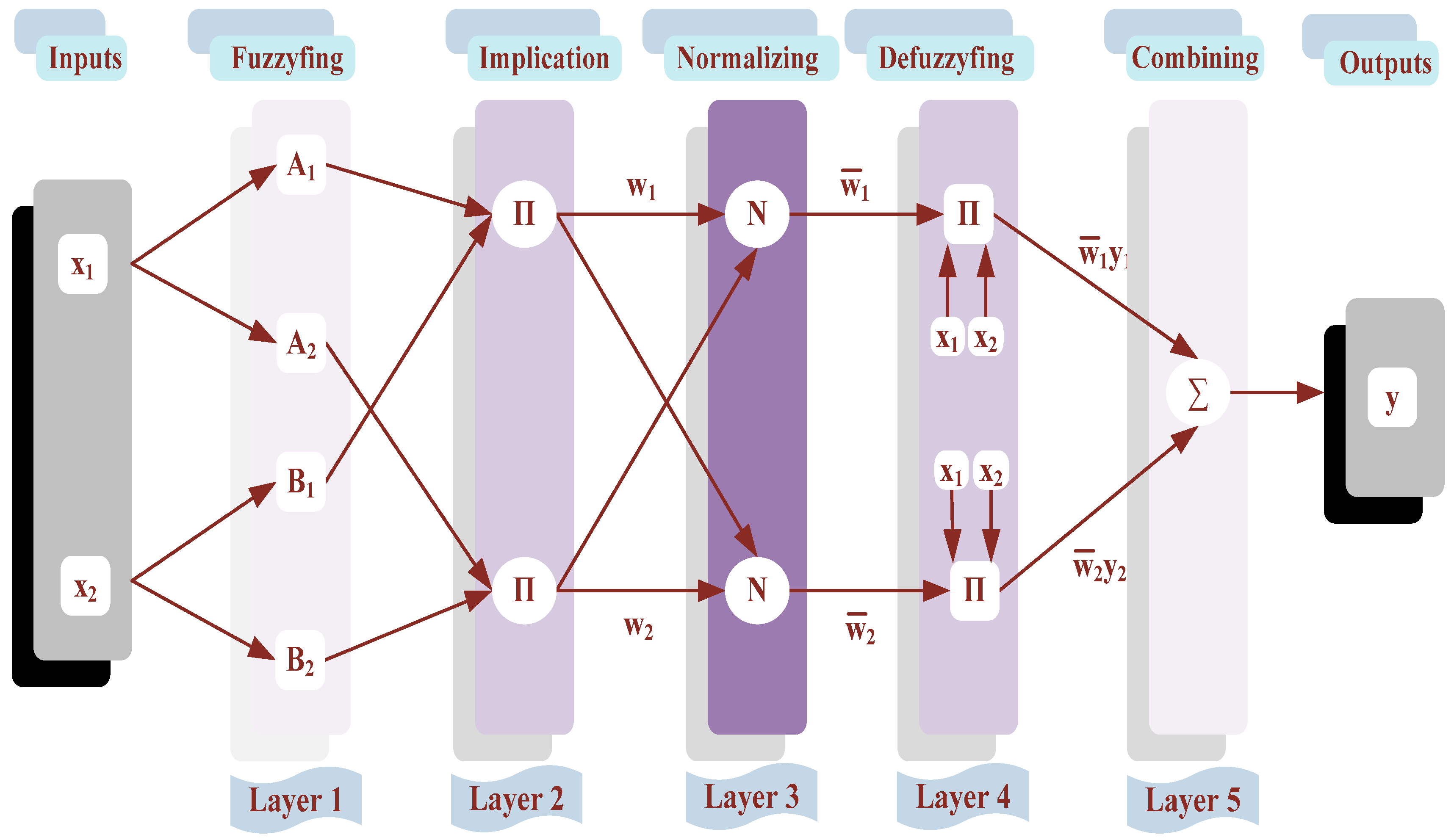
ANFIS is a combination intelligent technique that consists of both a fuzzy inference system and an artificial neural network. In addition, ANFIS is able to combine the advantages of both models into a unified solution technique to solve engineering problems [29]. A schematic diagram of the ANFIS architecture is depicted in Figure 2. ANFIS is a nonlinear model that describes the input–output relationship of a real system using the advantages of the learning capability of a neural network within the framework of a fuzzy system [30].
The basic rule of ANFIS with two inputs x1 and x2, and one output y can be defined as follows [30]:
Rule 1:
  if   x 1   is   A 1   and   x 2   is   B 1 ,   then   y 1 = p 1 x 1 +   q 1 x 2 +   r 1
Rule 2:
  if   x 1   is   A 2   and   x 2   is   B 2 ,   then   y 2 = p 2 x 1 +   q 2 x 2 +   r 2
Ai and Bi are the parameters of fuzzy sets of each input in part-if (premise part), while pi, qi, and ri are the linear parameters in part-then (consequent part).
The five layers comprising the ANFIS structure are involved for two inputs and a single output.
  • Fuzzifying Layer 1: Every node i in this layer is considered an adaptive node, where the output is defined as follows [30]:
    O i 1 = μ A i ( x 1 )   , for   i = 1 ,   2
    O i 1 = μ B i 2 ( x 2 )   , for   i = 3 ,   4
  • Implication Layer 2: The nodes are fixed nodes, labeled as π, and indicate that they act as a simple multiplier. The output of each node represents wi the firing strength of a rule and is formed based on incoming signals as follows [30]:
    O i 2 = w i = μ A i ( x 1 ) μ B i ( x 2 )   , for   i = 1 ,   2
  • Normalizing Layer 3: Every node in this layer is a fixed node labeled as N. The output signal w i ¯ of the ith node is calculated by the ratio of the ith rule’s firing strength to the sum of the firing strength for all rules as follows [30]:
    O i 3 = w i ¯ = w i w 1 +   w 2   , for   i = 1 ,   2
  • Defuzzifying Layer 4: Every node i in this layer is an adaptive node with a node function containing the resulting parameters (pi, qi, ri), and w i ¯ is a normalized firing strength from the previous layer as follows [30]:
    O i 4 = w i ¯ y i = w i ¯ ( p i x   +   q i y   +   r i )   , for   i = 1 ,   2
  • Combining Layer 5: This last layer contains a single fixed node labeled as Ʃ, which adds all the input signals to calculate the total final output as follows [30]:
    O i 5 = y = i ( w i ¯ y i ) = i w i y i i w i

Proposed PV Model Based on ANFIS

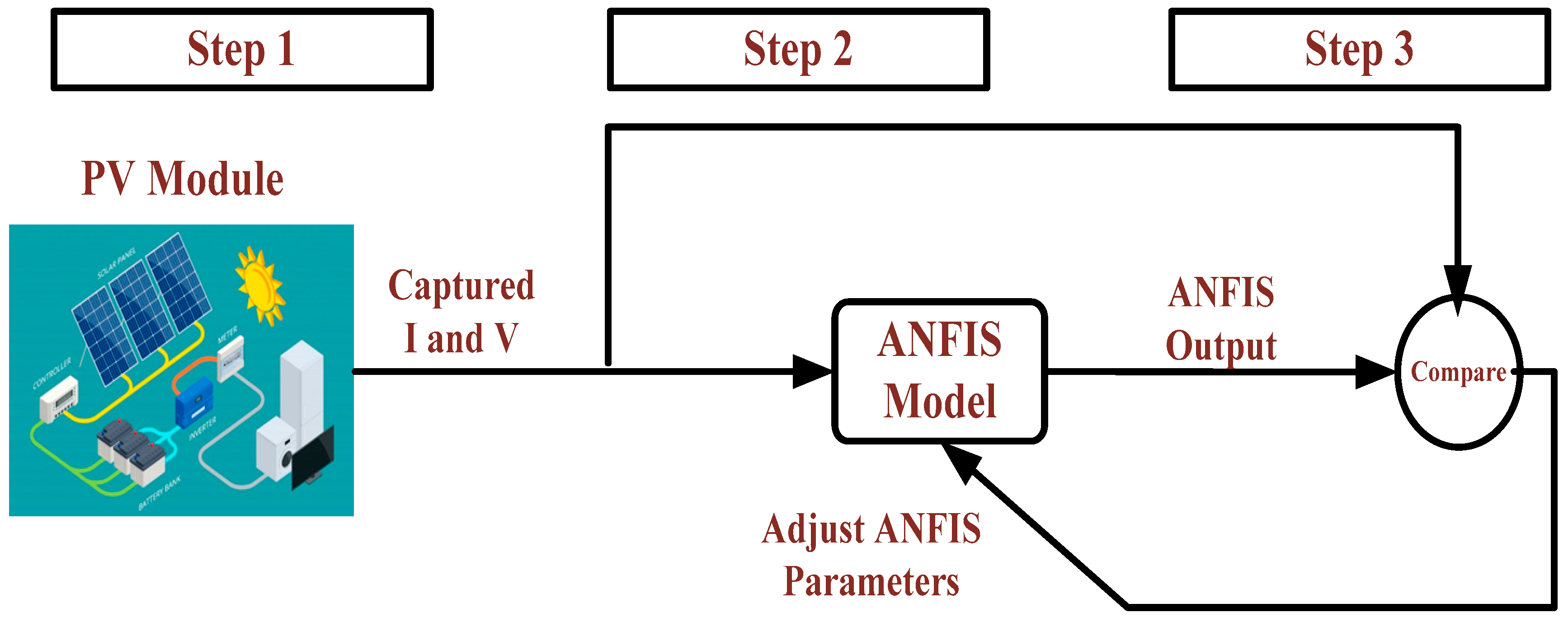
The proposed dynamic ANFIS PV model is based on learning the ANFIS model from the captured output current and voltage of the real PV module. Data are captured at a selected irradiance level and temperature. The real data used in this paper are the data of the PV module captured at a temperature of 25 °C and an irradiance level of 655 W/m2, which are used to learn the ANFIS model [24]. The learning method selected for ANFIS learning is a hybrid method between backpropagation for the parameters associated with the input membership functions and least-squares estimation for the membership functions of the output parameters. After learning the ANFIS model, the ANFIS output, which represents the output current of the PV module, is compared with the real output current, and the root mean square error (RMSE) is calculated using (9) [25] between the two compared values. The RMSE is one of the most commonly used measures for evaluating model quality. To compute the RMSE, the square of the difference between the real current (I) and the estimated ANFIS model output current for each data point is computed, then the means of these last computed values are computed. Based on the value of the calculated RMSE, the ANFIS parameters are readjusted to achieve the required value of the objective function. The main objective is to minimize this RMSE. The learning process is presented in Figure 3 and can be summarized as follows:
Step 1: Collect the required input and output data from the real PV system.
Step 2: Learn the ANFIS model based on the input and output data through the initial parameters for ANFIS.
Step 3: Compare the real output with the estimated output of the ANFIS. Based on the error, readjust the ANFIS parameters until the optimum ANFIS output is obtained.
RMSE = 1 N K = 1 N ( I   I ANFIS ) 2
where I and I ANFIS are the measured output current captured from the real system and the output current of the ANFIS model, respectively, and N is the number of the measured data.

4. Results

In this section, the steps of the designed ANFIS model are discussed. The ANFIS model accuracy is influenced by the three main parameters of the model. These parameters are number of MFs, MF type, and number of epochs. The effect of each parameter is tested individually, then the best choice is used in the final model. The initial values are as follows: number of MFs = 3; number of epochs = 5. The real data from the PV module captured at a temperature of 25 °C and an irradiance level of 655 W/m2 are used to learn the ANFIS model [24]. Model accuracy is tested by calculation of the RMSE and comparing for each test, as well as the absolute error. The absolute error is the absolute value between the estimated quantity and the real quantity. It is commonly used to measure the difference between the estimated and real values. The absolute error is calculated using (10) [25] between the output current captured from the real system and the output current from the ANFIS model and verified in different tests. All simulations are carried on MATLAB (R2016 a) based on a computer with an 8 GB RAM environment and with an Intel(R) Core(TM) i7–3520 M CPU @ 2.90 GHz.
  Absolut   error   of   current = ( I   I ANFIS ) 2

4.1. Performance of ANFIS at Different Types of MFs

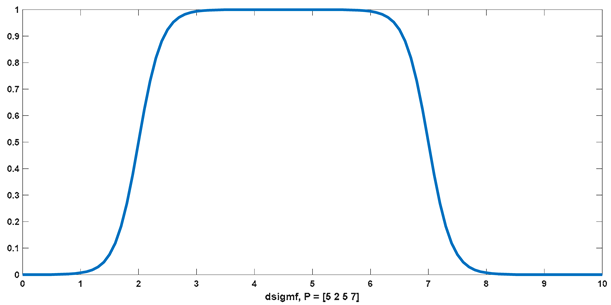
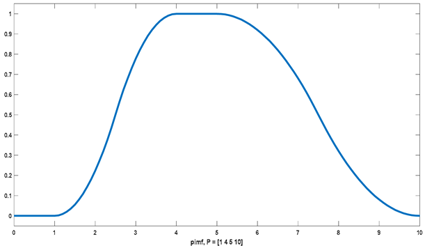
In this subsection, the ANFIS model is tested through different types of MFs. The initial values used for the number of MFs and number of epochs are 3 and 5, respectively. A list of each MF and obtained RMSE is presented in Table 1. The RMSE values are arranged in a descending sort, whereby the minimum RMSE is obtained by the difference between two sigmoidal MFs, as listed in the first row in Table 1, and the maximum RMSE is obtained by the product of two sigmoidal MFs, as listed in the final row. A description of the four best MFs is presented in Table 2. Table 2 presents the equation and shape of each MF. Each function has an independent variable (x) and some constants. The function output f(x) mainly depends on the value of (x). The shape of each function is based on the value and sign of the function’s constants such as a , b , c , d ,   and   σ . dsigmf has the best RMSE with the same initial values as the number of MFs and number of epochs when compared to the other MFs. The output current of the ANFIS model at different MFs and the real output current are compared and presented in Figure 4. The calculated absolute error of the output current at different MFs is presented in Figure 5.

4.2. Performance of ANFIS at Different Numbers of Epochs

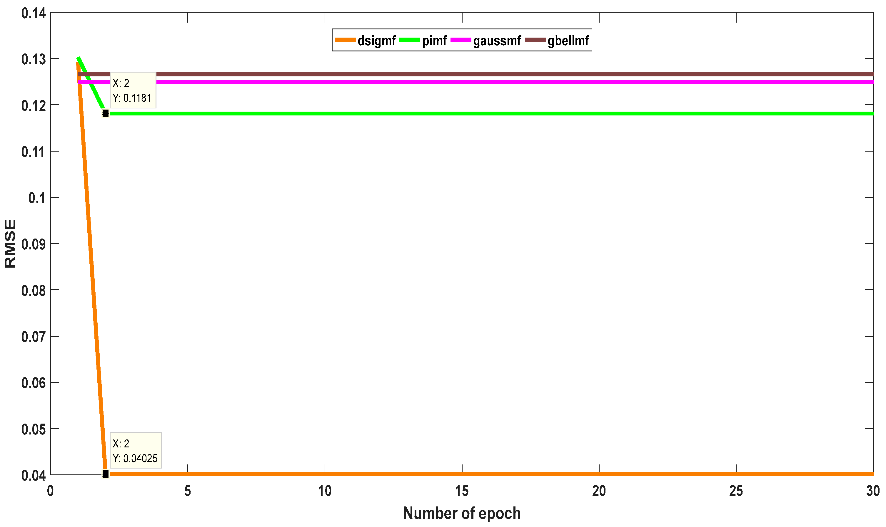
In this subsection, the ANFIS model is tested through different numbers of epochs. The initial value used for the number of MFs is 3. This test aims to test the effect of increasing the number of learning epochs on the ANFIS model accuracy. The test is repeated with each MF by changing the number of epochs from 1 to 30. The RMSE value is recorded with each number of epochs and is presented in Figure 6. Figure 6 presents the test for the different MFs. From Figure 6, the RMSE reaches the steady state at Epoch 2 for dsigmf and pimf, but for the other MFs, the change in epoch does not have any effect on the RMSE. From this test, the optimum epoch number is selected to be 5 as the initial condition.

4.3. Performance of ANFIS at Different Numbers of MFs

In this subsection, the ANFIS model is tested through different numbers of MFs. The best value for the number of epochs to be used is 5. This test aims to test the effect of increasing the number of MFs on the ANFIS model accuracy. The test is repeated with each MF by changing the number of MFs from 3 (initial value) to 150 MF. The maximum number of MFs (150) is selected, as all the four MFs compared reach the steady state at this limit. The RMSE value is recorded with each number of MFs and presented and discussed for each type of MF individually.

4.3.1. dsigmf

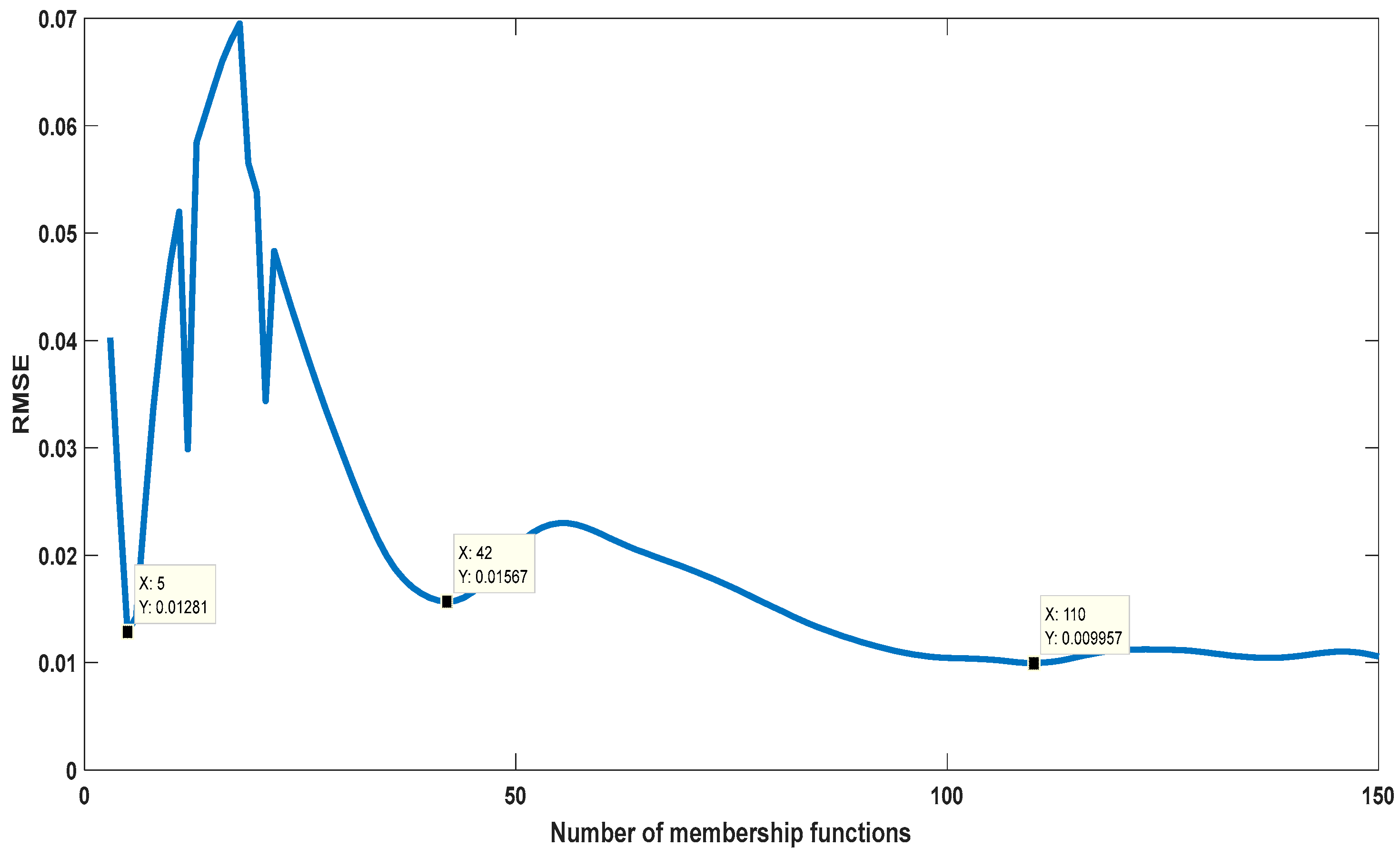
In this test, the MF type selected for the input variables is dsigmf. Figure 7 presents a curve for the obtained RMSE between the real output current and ANFIS model output. The points at which the better RMSE values are obtained are highlighted in the figure for each test and can be described as follows: the first best RMSE value = 0.01281, obtained when the number of MFs = 5. Increasing the number of MFs to more than 5 has a bad effect on the RMSE until the first peak when the number of MFs = 42 with the RMSE = 0.0156, which is still better than the first value. The best RMSE is obtained when the number of MFs = 110 (0.009957), as shown in Figure 7. From this test, dsigmf is selected as the input variable. The ANFIS model is more suitable for the real system when the number of MFs = 110.

4.3.2. pimf

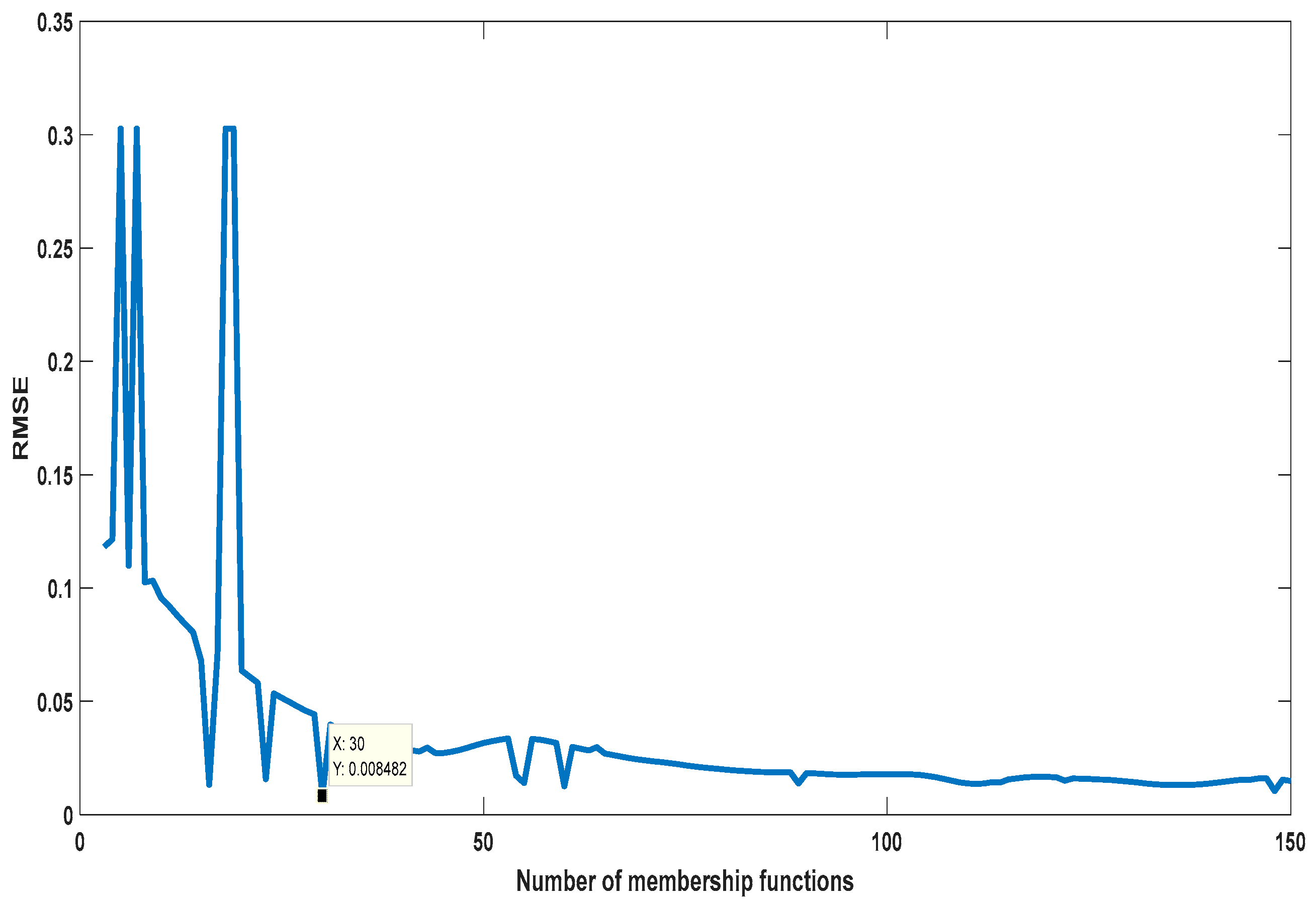
In this test, the selected MF type for the input variables is Pimf. Figure 8 presents the curve for the obtained RMSE between the real output current and the ANFIS model output. The points at which the better RMSE values are obtained are highlighted in the figure for each test and can be described as follows: different peaks are obtained with the increasing number of MFs, but the best RMSE value (0.008482) is obtained when the number of MFs = 30. Other peaks have an RMSE value greater than that obtained when the number of MFs = 30, as presented in Figure 8.

4.3.3. gaussmf

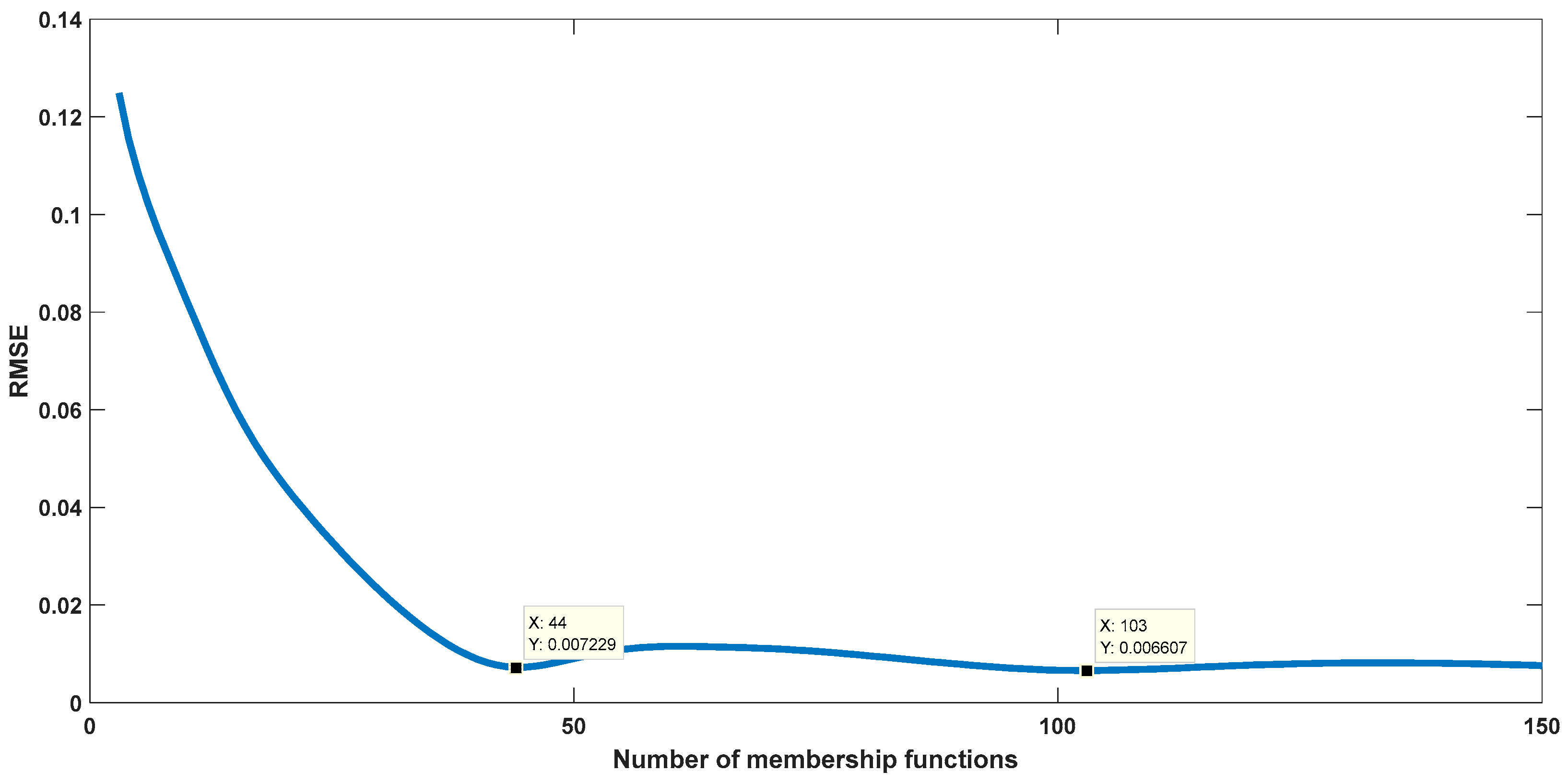
In gaussmf, the first best RMSE value = 0.007229 is obtained when the number of MFs = 44. The increasing number of MFs to more than 44 has a bad effect on the RMSE until the best RMSE when the number of MFs = 103 (0.0096607) is obtained, as shown in Figure 9.

4.3.4. gbellmf

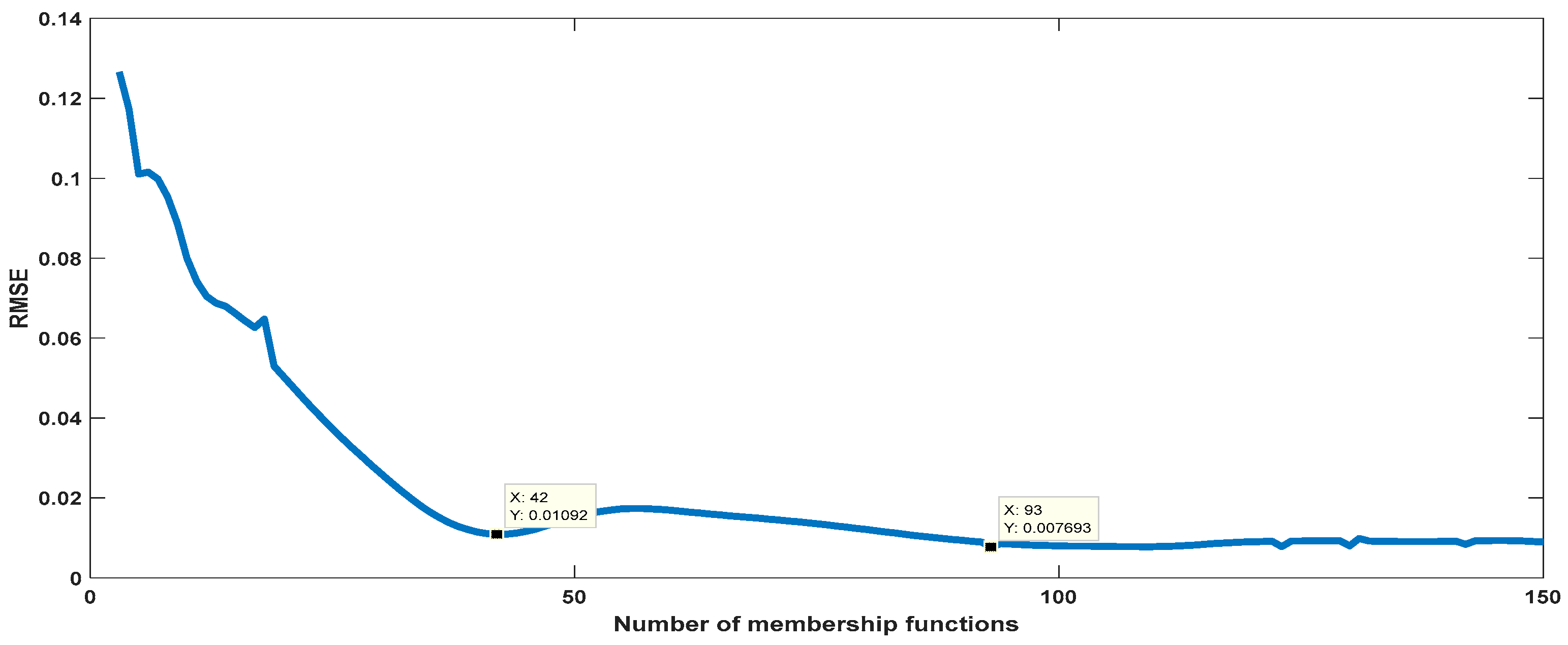
The behavior of the gbellmf function is similar to gaussmf but with different values. In gbellmf, the first best RMSE value = 0.01092 is obtained when the number of MFs = 42. Increasing the number of MFs to more than 42 has a bad effect on the RMSE until the best RMSE when the number of MFs = 93 (0.007693) is obtained, as shown in Figure 10.

4.4. Comparative Study and Discussion

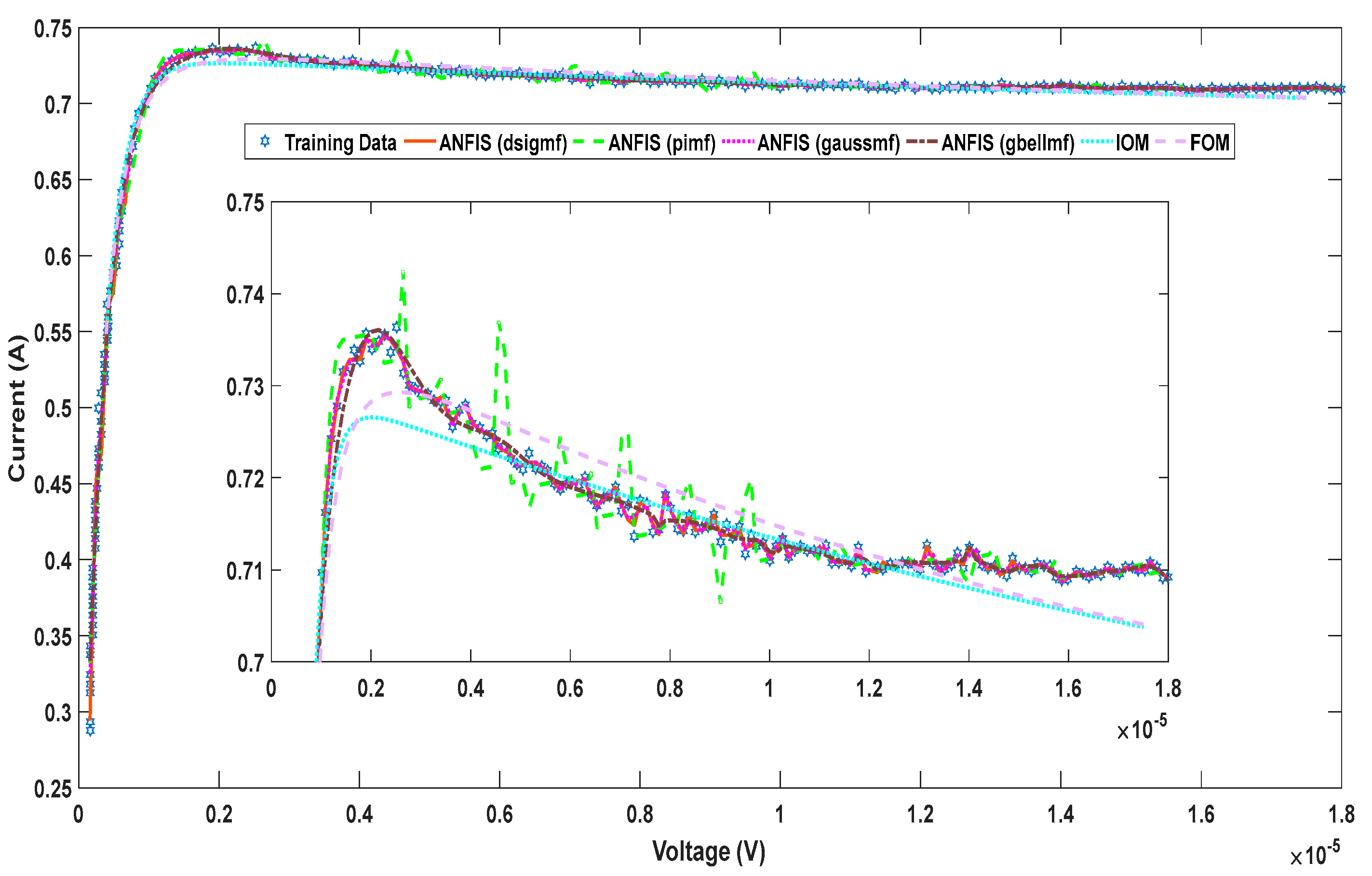
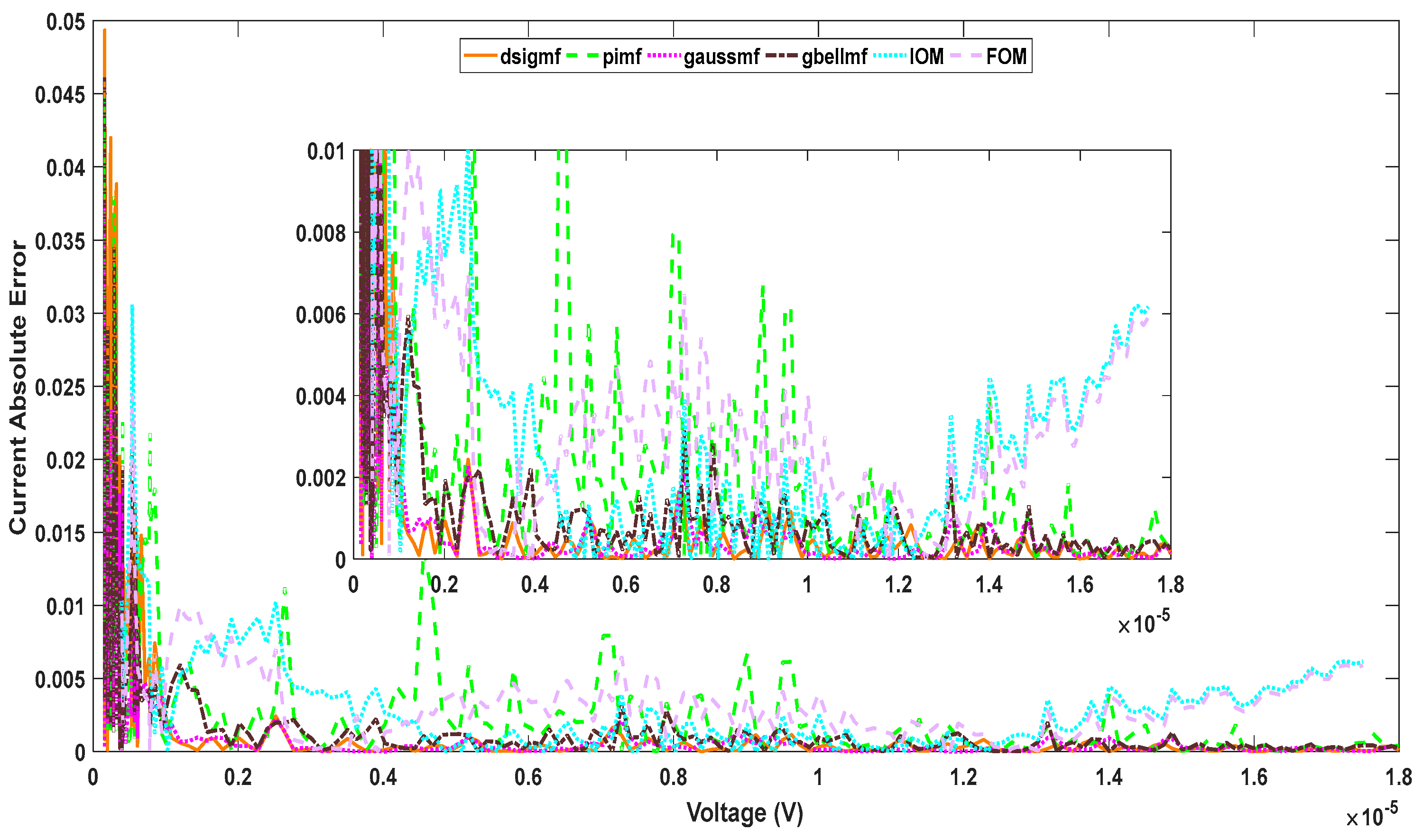
The ANFIS model accuracy is tested in three tests, each of which is concerned with discussing the effect of one of the three main parameters of the ANFIS design. The first test examined the effect of changing the MF type. The second and third tests consider the first best MFs. The first four best MFs started with the best MF are dsigmf, pimf, gaussmf, and gbellmf. The second test concerns selecting the optimum number of epochs to use in the other tests. The optimum number is chosen to be five epochs, as no change in RMSE value is recorded for numbers larger than five in all compared MFs. The third test concerns examining the effect of increasing the number of MFs on the ANFIS model accuracy. From the obtained results for the four compared MFs, although increasing the number of MFs has a variable effect on the RMSE value, the main behavior is the decrease in the RMSE, as well as the model accuracy. Better RMSE values are obtained at a high number of MFs. The limit of the high value of MFs changes with the type of MF, as shown in Table 3. Table 3 presents each MF and the number of MFs that achieve the best RMSE. Although the best RMSE when the number of MFs = 3 is obtained using dsigmf (see Table 1), the best RMSE is obtained using gaussmf when the number of MFs = 103. The lowest MFs number (30) is obtained using pimf with a satisfactory RMSE; thus, it takes advantage of the simplest model. The output current of the ANFIS model at different MFs with the best number of MFs and the real output current are compared and presented in Figure 11. The calculated absolute error of the output current at different MFs with the best number of MFs is presented in Figure 12. In order to compare the ANFIS model with the classical models in the literature, the RMSEs obtained by [23] for the IOM and FOM are presented in Table 3. The obtained RMSEs using gaussmf and gbellmf are better than both the IOM and FOM. For comparison, the output current and the current absolute error of IOM and FOM are presented in Figure 11 and Figure 12, respectively.

5. Conclusions

A novel dynamic PV model based on ANFIS is proposed in this paper. The proposed model has been designed considering different effective parameters in ANFIS. The design procedure tests different MF types. Based on the comparison of the obtained RMSE for all MF types, the best four types are dsigmf, pimf, gaussmf, and gbellmf, which are used in the other design steps. The proposed model has been designed to simulate a real PV module. The design of the ANFIS model includes testing different numbers of epochs and different numbers of MFs. The best ANFIS design for this PV module is a Gaussian MF with 103 MFs. The obtained RMSE is 0.0066, which is better than the RMSE obtained by the classical dynamic models (IOM and FOM). The output current from the ANFIS model is compared in case of using different number of MFs, to determine the best number of MFs. The output current from the ANFIS model is also compared with the output current obtained from the IOM and FOM. The output current obtained from the Gaussian MFs is more suitable than the real output current; moreover, it has a lower current absolute error curve in comparison to the other models. From the obtained results, the accuracy of the dynamic PV model based on ANFIS is better than the other classical dynamic PV models, which is simply due to the absence of complex mathematical equations. For future work, the proposed methodology in the ANFIS design can be used to develop an ANFIS model for complex dynamic PV systems, as well as optimize the best design parameters of the ANFIS model.

Author Contributions

Conceptualization, A.R. and S.K.; methodology, I.H. and A.M.A.; software, A.R. and S.K.; validation, I.H. and A.M.A.; formal analysis, A.R. and S.K.; investigation, I.H. and A.M.A.; resources, A.R. and S.K.; data curation, I.H. and A.M.A.; writing—original draft preparation, A.R. and S.K.; writing—review and editing, I.H. and A.M.A.; visualization, I.H. and A.M.A.; supervision, A.R. and S.K.; project administration, I.H. and A.M.A. All authors have read and agreed to the published version of the manuscript.

Funding

This research was funded by the Deputyship for Research & Innovation, Ministry of Education in Saudi Arabia through the project number “IF_2020_NBU_415”.

Institutional Review Board Statement

Not applicable.

Informed Consent Statement

Not applicable.

Data Availability Statement

Not applicable.

Acknowledgments

The authors extend their appreciation to the Deputyship for Research & Innovation, Ministry of Education in Saudi Arabia for funding this research work through the project number “IF_2020_NBU_415”. The authors gratefully thank the Prince Faisal bin Khalid bin Sultan Research Chair in Renewable Energy Studies and Applications (PFCRE) at Northern Border University for their support and assistance.

Conflicts of Interest

The authors declare no conflict of interest.

References

  1. Kumar, R.; Khan, F.U.; Sharma, A.; Aziz, I.B.A.; Poddar, N.K. Recent Applications of Artificial Intelligence in the Detection of Gastrointestinal, Hepatic and Pancreatic Diseases. Curr. Med. Chem. 2022, 29, 66–85. [Google Scholar] [CrossRef] [PubMed]
  2. Pujari, V.; Sharma, Y.; Burate, O. Application in artificial intelligence. Contemp. Res. 2021, 39–44, ISSN 2231-2137. [Google Scholar]
  3. Xiao, Z.; Hua, H.; Cao, J. Overview of the Application of Artificial Intelligence in Energy Internet. Electr. Power Constr. 2019, 40, 63–70. [Google Scholar]
  4. Mellit, A. Recent Applications of Artificial Intelligence in Fault Diagnosis of Photovoltaic Systems. In A Practical Guide for Advanced Methods in Solar Photovoltaic Systems; Springer: Berlin/Heidelberg, Germany, 2020; Volume 128. [Google Scholar]
  5. Uthathip, N.; Bhasaputra, P.; Pattaraprakorn, W. Application of ANFIS Model for Thailand’s Electric Vehicle Consumption. Comput. Syst. Sci. Eng. 2022, 42, 69–86. [Google Scholar] [CrossRef]
  6. Xue-bo, J.; Jiang-feng, W.; Hui-yan, Z.; Li-hong, C. ANFIS model for time series prediction. Appl. Mech. Mater. 2013, 386, 1411–1414. [Google Scholar]
  7. Armaghani, D.J.; Asteris, P.G. A comparative study of ANN and ANFIS models for the prediction of cement-based mortar materials compressive strength. Neural Comput. Appl. 2021, 33, 4501–4532. [Google Scholar] [CrossRef]
  8. Tiwari, S.; Babbar, R.; Kaur, G. Performance Evaluation of Two ANFIS Models for Predicting Water Quality Index of River Satluj (India). Adv. Civ. Eng. 2018, 2018, 8971079. [Google Scholar] [CrossRef] [Green Version]
  9. Kurtgoz, Y.; Deniz, E. Comparison of ANN, Regression Analysis, and ANFIS Models in Estimation of Global Solar Radiation for Different Climatological Locations. In Exergetic, Energetic and Environmental Dimensions; Elsevier: Amsterdam, The Netherlands, 2018; Chapter 1.8; pp. 133–148. [Google Scholar]
  10. Naresh, C.; Bose, P.S.C.; Rao, C.S.P. Artificial neural networks and adaptive neuro-fuzzy models for predicting WEDM machining responses of Nitinol alloy: Comparative study. SN Appl. Sci. 2020, 2, 314. [Google Scholar] [CrossRef] [Green Version]
  11. Gadeo-Martos, M.A.; Yuste-Delgado, A.J.; Cruz, F.A.; Prieto, J.F.; Bago, J.C. Modeling a High Concentrator Photovoltaic Module Using Fuzzy Rule-Based Systems. Energies 2019, 12, 567. [Google Scholar] [CrossRef] [Green Version]
  12. Buriboev, A.; Kang, H.K.; Ko, M.C.; Oh, R.; Abduvaitov, A.; Jeon, H.S. Application of Fuzzy Logic for Problems of Evaluating States of a Computing System. Appl. Sci. 2019, 9, 3021. [Google Scholar] [CrossRef] [Green Version]
  13. Badde, D.S.; Gupta, A.k.; Patki, V.K. Comparison of Fuzzy Logic and ANFIS for Prediction of Compressive Strength of RMC. IOSR J. Mech. Civil. Eng. 2013, 3, 7–15. [Google Scholar]
  14. Aengchuan, P.; Phruksaphanrat, B. Comparison of fuzzy inference system (FIS), FIS with artificial neural networks (FIS + ANN) and FIS with adaptive neuro-fuzzy inference system (FIS + ANFIS) for inventory control. J. Intell. Manuf. 2018, 29, 905–923. [Google Scholar] [CrossRef]
  15. Lincy Luciana, M.; Senthil Kumar, R. Comparison Analysis of Fuzzy Logic and Anfis Controller for Mitigation of Harmonics. In Proceedings of the 2018 4th International Conference on Electrical Energy Systems (ICEES), Chennai, India, 7–9 February 2018; 2018; pp. 578–583. [Google Scholar] [CrossRef]
  16. Nigam, A.; Sharma, K.K. Modeling Approach for Different Solar PV System: A Review. In Advances in Systems, Control and Automations; Lecture Notes in Electrical Engineering; Bhoi, A.K., Mallick, P.K., Balas, V.E., Mishra, B.S.P., Eds.; Springer: Singapore, 2021; Volume 708. [Google Scholar] [CrossRef]
  17. Ramadan, A.; Kamel, S.; Ibrahim, A.A. Parameters Estimation of Photovoltaic Cells Using Self-adaptive Multi-population Rao Optimization Algorithm. Aswan Univ. J. Sci. Technol. 2021, 1, 26–40. [Google Scholar]
  18. Ramadan, A.; Kamel, S.; Taha, I.B.M.; Tostado-Véliz, M. Parameter Estimation of Modified Double-Diode and Triple-Diode Photovoltaic Models Based on Wild Horse Optimizer. Electronics 2021, 10, 2308. [Google Scholar] [CrossRef]
  19. Castro, R.; Silva, M. Experimental and Theoretical Validation of One Diode and Three Parameters–Based PV Models. Energies 2021, 14, 2140. [Google Scholar] [CrossRef]
  20. Ramadan, A.; Kamel, S.; Khurshaid, T.; Oh, S.; Rhee, S.-B. Parameter Extraction of Three Diode Solar Photovoltaic Model Using Improved Grey Wolf Optimizer. Sustainability 2021, 13, 6963. [Google Scholar] [CrossRef]
  21. El-Dabah, M.A.; El-Sehiemy, R.; Becherif, M.; Ebrahim, M.A. Parameter estimation of triple diode photovoltaic model using an artificial ecosystem-based optimizer. Int Trans. Electr. Energ. Syst. 2021, 31, e13043. [Google Scholar] [CrossRef]
  22. Abdelghany, R.Y.; Kamel, S.; Ramadan, A.; Sultan, H.; Rahmann, C. Solar Cell Parameter Estimation Using School-Based Optimization Algorithm. In Proceedings of the IEEE International Conference on Automation/XXIV Congress of the Chilean Association of Automatic Control (ICA-ACCA), Santiago, Chile, 22–26 March 2021. [Google Scholar]
  23. Ramadan, A.; Kamel, S.; Hassan, M.H.; Tostado-Véliz, M.; Eltamaly, A.M. Parameter Estimation of Static/Dynamic Photovoltaic Models Using a Developed Version of Eagle Strategy Gradient-Based Optimizer. Sustainability 2021, 13, 13053. [Google Scholar] [CrossRef]
  24. Yousri, D.; Allam, D.; Eteibaa, M.B.; Suganthanb, P.N. Static and dynamic photovoltaic models’ parameters identification using Chaotic Heterogeneous Comprehensive Learning Particle Swarm Optimizer variants. Energy Convers. Manag. 2019, 182, 546–563. [Google Scholar] [CrossRef]
  25. Ramadan, A.; Kamel, S.; Hassan, M.H.; Ahmed, E.M.; Hasanien, H.M. Accurate Photovoltaic Models Based on an Adaptive Opposition Artificial Hummingbird Algorithm. Electronics 2022, 11, 318. [Google Scholar] [CrossRef]
  26. Go, S.-E.; Choi, J.-O. Design and Dynamic Modelling of PV-Battery Hybrid Systems for Custom Electromagnetic Transient Simulation. Electronics 2020, 9, 1651. [Google Scholar] [CrossRef]
  27. Batzelis, E.I.; Anagnostou, G.; Cole, I.R.; Betts, T.R.; Pal, B.C. A State-Space Dynamic Model for Photovoltaic Systems with Full Ancillary Services Support. IEEE Trans. Sustain. Energy 2018, 10, 1399–1409. [Google Scholar] [CrossRef] [Green Version]
  28. Parida, S.M.; Rout, P.K. Differential evolution with dynamic control factors for parameter estimation of photovoltaic models. J. Comput. Electron. 2021, 20, 330–343. [Google Scholar] [CrossRef]
  29. Bensaber, B.A.; Diaz, G.P.; Lahrouni, Y. Design and modeling an Adaptive Neuro-Fuzzy Inference System (ANFIS) for the prediction of a security index in VANET. J. Comput. Sci. 2020, 47, 101234. [Google Scholar] [CrossRef]
  30. Haznedar, B.; Kalinli, A. Training ANFIS structure using simulated annealing algorithm for dynamic systems identification. Neurocomputing 2018, 302, 66–74. [Google Scholar] [CrossRef]
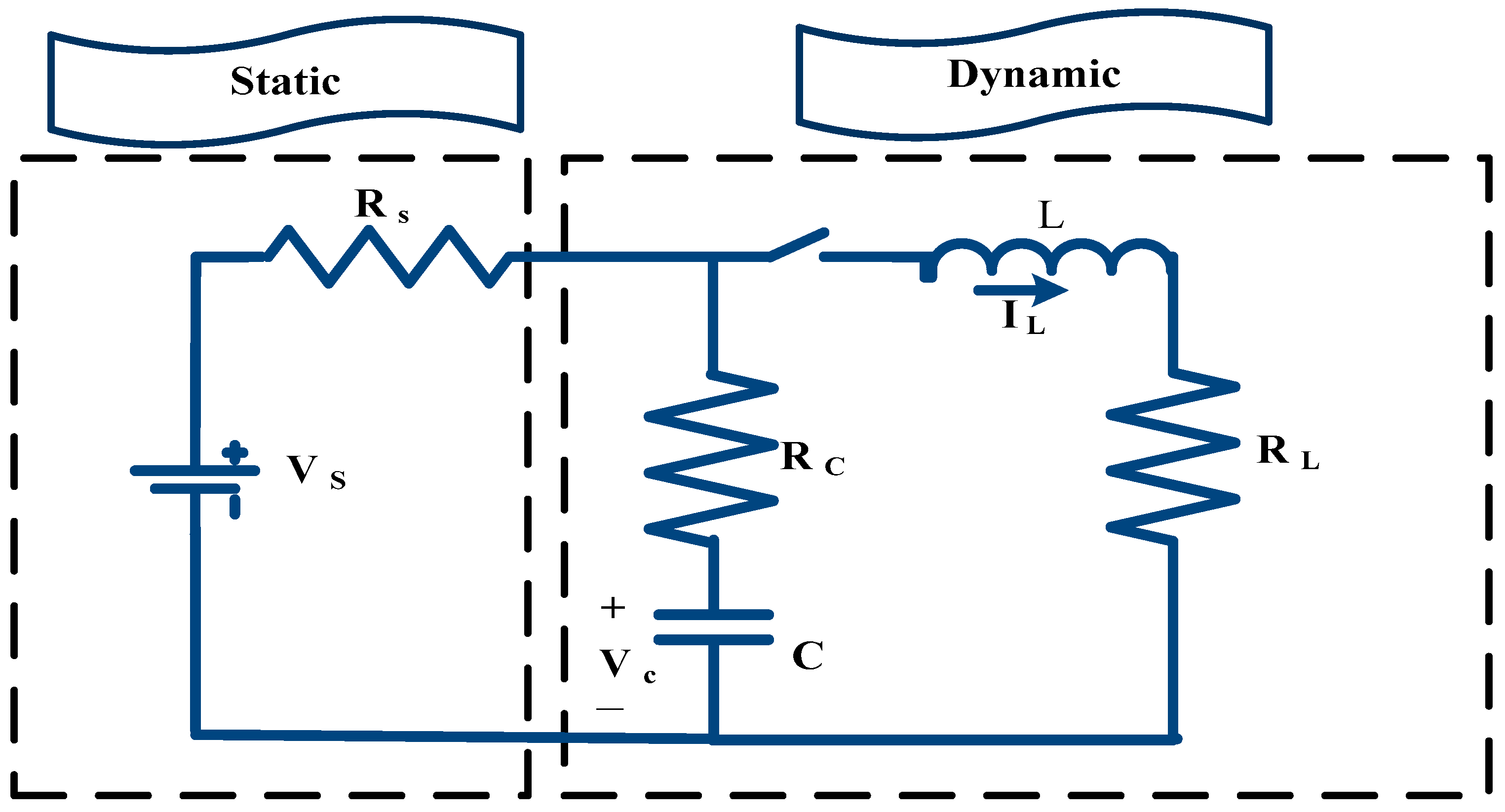
Figure 1. Integral-order model for PV system.
Mathematics 10 01286 g001
Figure 2. Schematic diagram of ANFIS architecture.
Mathematics 10 01286 g002
Figure 3. Learning process of PV model based on ANFIS.
Mathematics 10 01286 g003
Figure 4. Output current of the real system and ANFIS model at different MFs.
Mathematics 10 01286 g004
Figure 5. Absolute error between the output current of the real system and ANFIS model at different MFs.
Mathematics 10 01286 g005
Figure 6. RMSE values for the ANFIS model at different MFs and different numbers of epochs.
Mathematics 10 01286 g006
Figure 7. RMSE values for the ANFIS model at different numbers of MFs with dsigmf.
Mathematics 10 01286 g007
Figure 8. RMSE values for the ANFIS model at different numbers of MFs with pimf.
Mathematics 10 01286 g008
Figure 9. RMSE values for the ANFIS model at different numbers of MFs with gaussmf.
Mathematics 10 01286 g009
Figure 10. RMSE values for the ANFIS model at different numbers of MFs with gbellmf.
Mathematics 10 01286 g010
Figure 11. Output current of the real system and ANFIS model at different MFs with the best number of MFs.
Mathematics 10 01286 g011
Figure 12. Absolute error between the output current of the real system and ANFIS model at different MFs with the best number of MFs.
Mathematics 10 01286 g012
Table 1. MF type and obtained RMSE.
MF TypeRMSE
Difference between two sigmoids (dsigmf)0.04025089
Π-shaped (pimf)0.11812001
Symmetric Gaussian (gaussmf)0.12486303
Generalized bell-shaped (gbellmf)0.12657520
Gaussian combination (gauss2 mf)0.12901611
Product of two sigmoidal (psigmf)0.12927727
Trapezoidal-shaped (trapmf)0.34173833
Table 2. Description of MF types.
MF TypeEquationShape
dsigmfsigmf
f ( x ; a , c ) = 1 1 +   e a ( x c )
dsigmf
f ( x ; a 1 , c 1 , a 2 , c 2 ) = f ( x ; a 1 , c 1 ) f ( x ; a 2 , c 2 )
Mathematics 10 01286 i001
pimf f ( x ; a , b , c , d ) = { 0 , x a 2 ( x a b a ) 2 , a x a + b 2 1 2 ( x b b a ) 2 , a + b 2 x b 1 , b x c 1 2 ( x c d c ) 2 , c x c + d 2 2 ( x d d c ) 2 , c + d 2 x d 0 , d x } Mathematics 10 01286 i002
gaussmf f ( x ; σ , c ) = e ( x c ) 2 2 σ 2 Mathematics 10 01286 i003
gbellmf f ( x ; a , b , c ) = 1 1 + | x c a | 2   b Mathematics 10 01286 i004
Table 3. RMSE for each MF type with the best number of MFs.
MF TypedsigmfpimfgaussmfgbellmfIOM [23]FOM [23]
Best number of MF1103010393------
RMSE0.0099570.0084820.0066070.007690.0082590.007951
Publisher’s Note: MDPI stays neutral with regard to jurisdictional claims in published maps and institutional affiliations.