Abstract
This study investigates a supply chain of fresh produce with consideration of option contracts and where stochastic market demand depends on freshness-keeping effort. Firstly, we investigate a benchmark scenario of an integrated supply chain with freshness effort and consideration of decreases in both the quality and quantity of produce while in the supply chain. Secondly, we introduce call, put, and bidirectional option contracts to mitigate risks of the retailer. A call option contract can reduce the underage risk, while a put option contract can reduce the overage risk, and a bidirectional option contract can reduce bilateral risks. We derive the optimal ordering decisions and freshness-keeping effort for a retailer in a supply chain of fresh produce with option contracts, and the conditions for achieving coordination of the supply chain. We find that the bidirectional option results in the highest option price and lowest option order quantity, while the call option results in the lowest initial order quantity and the put option results in the highest initial order quantity. Finally, numerical examples are given to demonstrate the impacts of various parameters on optimal decision-making. This paper provides managerial insights for reducing risk in fresh produce supply chains.
MSC:
90B06
1. Introduction
Fresh produce, such as vegetables, fruits, meat, eggs, milk and seafood, plays an increasingly crucial role in people’s daily life (Wang and Chen, 2016 [1]). As a perishable product, fresh produce has a short shelf life, in addition to long lead times, high freshness requirements, large circulation losses, and almost zero salvage value at the end of the selling season. Its production is regional and seasonal, while its consumption is global and regular (Wang and Chen, 2021 [2]). Therefore, efficient supply chains are required to transport fresh produce from its origins to different destinations, some of them distant. However, unlike non-perishable goods, such as industrial products and consumer electronics, fresh produce easily suffers reductions in quantity and quality during transportation in the supply chain, resulting in significant losses. For instance, retailers in advanced Western economies can lose nearly 15% of their fresh produce to spoilage and damage. In China, the annual circulation loss of fruits and vegetables is about 30% of annual production (Xiao and Chen, 2012 [3]). Furthermore, the management of fresh produce supply chains is challenging due to random yields, stochastic demands and supply price fluctuations.
Cai et al. (2010) [4] pointed out that fresh products are subject to both “quantity loss” and “quality drop” during logistics and transportation, which can affect the amount and freshness of products, respectively, that reach the target market. Hence, preventing the deterioration of fresh produce is an important priority for suppliers and retailers, especially when the long-distance logistics and transportation is involved in the supply chain. For this reason, perishable fresh produce needs to be transported through cold chains in the process of circulation to maintain freshness and quantity during the logistics and sales processes to optimise profits. This effort to maintain the freshness of fresh produce is defined as “freshness-keeping effort”. Better packaging and cooling facilities and faster transportation can help reduce losses but increase the cost of the freshness-keeping effort to the supplier or the retailer (Wu et al., 2015 [5]). While increased freshness-keeping effort can maintain the quality of fresh produce at a higher price, supply chain members need to consider the trade-off between cost and profit.
In traditional supply chain management, retailers face the risks of underage and overage. Many studies have shown that a wholesale price contract cannot coordinate a supply chain that is decentralized. In the newsvendor model, a revenue-sharing contract is equivalent to a buyback contract, which is equivalent to a price discount contract in pricing analysis. Compared with a wholesale price contract, a revenue-sharing contract is slightly better (Cachon and Lariviere, 2005 [6]) in coordinating a supply chain. In recent years, the flexibility of option contracts has received theoretical attention from scholars who have utilized option derivatives to hedge the risks associated with supply chain uncertainty. They have gradually introduced option contracts into agricultural supply chains to reduce demand uncertainty risk. Option contracts are being used by a growing number of Chinese companies (e.g., the food processing, automobile, and high-tech industries) to mitigate the risks of unpredictably high demand, fluctuating pricing, and unreliable supplies (Chen et al., 2014 [7]). For instance, option contracts have been used in the fruit supply chains of Australian supermarkets (Wan et al., 2021 [8]). In addition, some flower operating companies in the Hainan province of China have provided flower options for international customers. Customers can pay 5% of the option price for a certain number of flowers before they are marketed, and then pay the remaining 95% at a pre-negotiated exercise price after the flowers are marketed. (Wang and Chen, 2016 [1]).
Option contracts provide a right (not an obligation) to the retailer to buy one more unit of fresh produce by a certain date at a pre-negotiated exercise price, subject to an advance payment of the option premium to the supplier. This contract brings flexibility to the retailer without harming the supplier. Option contracts have been proved in academic research to alleviate the impact of stochastic demand and decrease losses in the process of circulation (Wang and Chen, 2016 [1]). Call, put, and bidirectional options are the three types of options. A buyer can purchase a certain number of options from the provider who offers options by paying a retention fee before the demand is realized. After the demand is realized, the buyer has a right, but not an obligation, to exercise the option at a pre-negotiated price according to the reserved quantity or actual demand, whichever is lower. As one of the most commonly used instruments to hedge the risk of underage, the call option gives the buyer the right to reorder products from the supplier when the realized demand is high. Many scholars have thoroughly studied optimal ordering strategies and production decisions [1,7,9,10,11,12]. The put option allows a buyer to return unsold products to the supplier to reduce losses when the realized demand is low (Chen and Parlar, 2007 [13]). Some scholars have introduced the bidirectional option, which can be exercised as either call or put options, in order to improve the supply chain flexibility. Therefore, the bidirectional option not only ensures the supply of the buyer’s demand but also provides the buyer with supply flexibility (Chen et al., 2017 [14]; Wang et al., 2019 [15]). Yang et al. (2017) [16] compared and analysed the retailer’s optimal ordering decisions under a wholesale price contract and call, put, and bidirectional option contracts. Studies have found obvious differences in the exercise conditions and functions of various option contracts. How these similarities and differences affect the supply chain deserves our further study.
This paper establishes a newsvendor model based on option contracts to study the retailer’s optimal ordering decisions in a fresh produce supply chain, where circulation loss and freshness are dependent on the freshness-keeping effort. Three essential questions remain to be answered:
- (1)
- What are the optimal ordering decisions and freshness-keeping effort of the retailer for each of the three option contracts in a supply chain of fresh produce?
- (2)
- Among the three option contracts, what are the differences in the optimal initial order quantity and optimal option order quantity for a supply chain of fresh produce when the retailer is dedicated to freshness-keeping effort?
- (3)
- What are the coordination conditions for each of the three option contracts?
Our contributions are as follows. Firstly, we simultaneously consider the quality drop and quantity losses of fresh produce in the circulation process. A freshness level index and effective supply rate are introduced to characterize the freshness and circulation loss of fresh produce, respectively. Secondly, we introduce call, put, and bidirectional option contracts to reduce the retailer’s risk and derive their optimal ordering decisions. In addition, we also compare initial order and option order quantities and option prices for call, put, and bidirectional option contracts.
The rest of this paper is arranged as follows. Section 2 reviews the related literature. The model description, assumptions and integrated system analysis are presented in Section 3. In Section 4, we analyse the optimal ordering decisions and optimal freshness-keeping effort levels of the fresh produce retailer under call, put and bidirectional option contracts. Numerical examples are presented in Section 5. We discuss and conclude our work as well as give possible further research directions in Section 6.
2. Literature Review
This study is particularly interested in two main research streams. One is on fresh produce supply chain management, which considers freshness-keeping effort, and the other is on supply chain contracts with options.
2.1. Fresh Produce Supply Chain Management and Freshness-Keeping Effort
Recently, the supply chain management of fresh produce has attracted widespread attention from academics. A great number of studies have considered the characteristics of the deterioration of fresh produce over time when investigating the ordering decisions of a fresh produce supply chain. Blackburn and Scudder (2009) [17] introduced the marginal value of time (MVT) metric into fresh produce supply chain management to characterize the deterioration of fresh produce over time. For fresh produce, Bai et al. (2008) [18] developed a multi-item shelf space allocation and inventory management system. They found that, compared with heuristic and meta-heuristic methods, hyper-heuristic methods are more effective at larger problem scales. Xiao and Chen (2012) [3] observed fresh produce quantity losses during transportation over a vast distance and evaluated pull and push models to derive the optimal ordering decision and pricing strategy for both members of the supply chain. They also suggested using a fixed inventory plus factor (FIPF) strategy to achieve Pareto improvement over the pull model and push model. Many perishable goods considered in quality and physical quantity, such as fresh produce and other food, deteriorate proportionally over time, according to Qin et al. (2014) [19]. Taking into account that perishable food demand is price-quality sensitive, Liu et al. (2015) [20] investigated the optimal joint pricing and preservation investment strategy of the retailer for a given initial inventory. He et al. (2019) [21] investigated a competitive online presale model of fresh produce, and compared and analysed the pricing strategies of online grocery and physical stores. Yu et al. (2019) [22] considered an organic food supply chain with supplier competition. They studied the effect of suppliers conducting organic certification on wholesale pricing strategies, and then studied the retailer’s supplier selection decisions and pricing strategies. Chakraborty et al. (2017) [23] focused on different kinds of three-level supply chain models under inflation for the non-instantaneous deteriorating items (e.g., fresh produce etc.) and the retailer has a pre-specified time to settle the account with the supplier. Garai and Garg (2019) [24] solved a multi-objective linear fractional inventory problem with a generalized intuitionistic fuzzy environment.
While the above studies have considered the characteristics of fresh produce that deteriorate over time, they have not considered the effect of freshness-keeping effort on quality and freshness. Cai et al. (2010) [4] pointed out that there are “quantity losses” and “quality drops” (where quality refers to freshness) during the transportation of fresh products, and that both retail price and freshness have an impact on market demand. To ensure higher earnings, supply chain members must reduce the rates of quality drop and quantity loss via freshness-keeping effort. Cai et al. (2010) [4] studied a fresh product supply chain consisting of a supplier and a distributor that undertakes freshness-keeping efforts to maintain the products’ quality and quantity. They investigated the distributor’s optimal ordering quantity, market price and effort level, as well as the supplier’s optimal wholesale price, and the coordination condition of the supply chain. Some literature (Cai et al., 2013 [25]; Wu et al., 2015 [5]; Yu and Xiao, 2017 [26]; Song and He, 2019 [27]) has considered fresh produce outsourcing issues with a third-party logistics service provider (3PL, TPLSP) whose cold-chain service has an impact on the quantity and quality of perishable products that can be sold. Optimal decisions for the three supply chain members were derived. They also designed coordinating mechanisms such, as freshness-keeping cost-sharing and revenue-sharing contracts, to coordinate the supply chain. Mohammadi et al. (2018) [28] developed a novel coordination mechanism called the revenue-and-preservation-technology-investment-sharing contract (RPTIS) based on preservation-technology investment to coordinate a fresh product supply chain. They found that RPTIS not only decreases the amount of waste but also increases the profits of independent fresh-product supply chain members. None of these studies, however, have considered option contracts for fresh produce supply chains. As mentioned above, option contracts have been applied in practice in the food processing industry and agriculture. It is very important and necessary to utilize the flexibility of option contracts to reduce risks of underage and overage in the supply chain of fresh produce.
2.2. Supply Chain Contracts with Options
Option contracts are divided into three types: call, put, and bidirectional, as mentioned before. Regarding supply chain contracts with call options, Zhao et al. (2010) [29] utilized a cooperative game method using option contracts to investigate supply chain coordination issues, and option contracts were shown to be effective in achieving supply chain coordination and Pareto improvement. Under various assumptions, Fu et al. (2012) [30], Lee et al. (2013) [9], and Luo et al. (2019) [31] studied optimal ordering decisions and optimal production policies in a multiple-supplier situation with a spot market. Gomez-Padilla and Mishina (2009) [32] considered the impacts of option contracts on supply chain members in cases of (1) multiple suppliers and one retailer and (2) one supplier and one retailer. Xu (2010) [33] studied the optimal production policies of the supplier and the optimal ordering decisions of the manufacturer in a supply chain consisting of the supplier with random yield and the manufacturer with stochastic demand based on option contracts. Chen and Shen (2012) [10] analysed a supply chain with service requirements and option contracts, and demonstrated that option contracts are beneficial to both members of the supply chain. Option contracts were incorporated into the relief material supply chain management by Liang et al. (2012) [34], and they studied the pricing strategies of supply chain members. Wang and Chen (2015) [11] studied the optimal ordering decisions and pricing strategies, and compared the difference between single ordering (when the retailer uses an option contract or a wholesale price contract to place an order) and mixed ordering (when the retailer places an order under an option contract and a wholesale price contract simultaneously) of call options in a newsvendor model with uncertain demand. Under asymmetric information of supply cost, Nosoohi and Nookabadi (2015) [35] investigated an outsourcing plan based on option contracts. Arani et al. (2016) [36] studied a coordination for a supply chain of retailer-manufacturer through a revenue-sharing option contract. They derived the optimal ordering quantity of the retailer and the optimal production quantity of the manufacturer under the Nash equilibrium. Cai et al. (2017) [37] investigated the relationship between option contracts and subsidy contracts based on a supply chain of vendor-managed inventory (VMI) under random yield. Hu et al. (2018) [38] investigated the coordination issue in a supply chain with option contracts and joint pricing, as well as optimized the order quantity, market price, option price, and option exercise price. In the scenario of price-dependent stochastic demand and the option of purchasing option contracts, Wang et al. (2017) [12] created a newsvendor model to explore how customer returns affect pricing strategies and ordering decisions of a firm. They calculated the optimal initial ordering quantity, option order quantity and market price for the retailer simultaneously. Luo and Chen (2015) [39] studied the impact of call options on a supply chain of supplier-manufacturer with random yield and a spot market. The conditions of supply chain coordination and Pareto improvement for both supply chain members were determined. Sharma et al. (2019) [40] studied the fairness concerns of chain members in an option supply chain, finding that under certain pricing conditions, the supply chain can be coordinated through an option contract. Biswas and Avittathur (2019) [41] demonstrated that options contracts coordinate single-supplier–multiple-buyer supply chain networks and can eliminate the channel conflict that stems from simultaneous price and inventory competition. This provides suppliers with greater flexibility in profit distribution compared to buyback contracts. Some scholars (Chen et al., 2014 [7]; Fan et al., 2020 [42]; Liu et al., 2020 [43]; Jia and Wang, 2022 [44]) have studied the option ordering decisions, option pricing strategies, and conditions of the coordination of risk-averse supply chain members under option contracts. Xue et al. (2018) [45] investigated how a core company uses option contracts and order-commitment contracts to mitigate the supply disruption risk. They derived the optimal production policies and optimal procurement strategies under these two types of contracts, as well as the optimal contract selection strategy of the core company. While research on put options is rare, to mitigate losses caused by low demand, Chen and Parlar (2007) [13] utilized put options in a supply chain with stochastic demand and a risk-averse newsvendor. Luo et al. (2018) [46] found that put options not only promote the ordering quantity of the manufacturer but also promote the production quantity of the supplier. When used in combination with a protocol, put options can coordinate the supply chain. Hu et al. (2019) [47] studied the conditions under which put option contracts coordinate a relief supply chain. They explained the superiority of put option contracts compared with wholesale price contracts and buyback contracts. Wang et al. (2019) [48] explored the effects of customer returns on ordering decisions and optimal pricing strategies under a put option contract, as well as the profits of the supplier and the retailer. They also discussed a coordination mechanism for the supply chain to ensure greater profits for the supplier and the retailer. Chen et al. (2020) [49] derived the optimal ordering decisions and production policies for a supply chain with put options under a service level constraint. They also found that retailers can make greater profits and offer higher service levels by using a put option. Guo et al. (2021) [50] proposed a flexible return policy under stochastic demand, where the retailer can independently select the return quantity through put options after the end of the selling season. They estimated the optimal pricing strategies and ordering decisions of the supply chain members. Bakhshi and Heydari (2021) [51] analysed a two-echelon reverse supply chain (RSC) that included a re-manufacturer facing uncertainty in remanufacturing capabilities. Regarding supply chain contracts with bidirectional options, Zhao et al. (2013) [52] derived the retailer’s optimal initial ordering strategy and optimal option ordering strategy in a supply chain with a bidirectional option contract. They further discussed how the bidirectional option contract achieves supply chain coordination. In the presence of a service requirement and bidirectional option contract, Chen et al. (2017) [14] showed that bidirectional option contracts are beneficial to both members of the supply chain, and proposed a coordination condition of distribution-free to achieve Pareto improvement. Wang et al. (2019) [15] investigated the impact of customer returns and a bidirectional option contract on a newsvendor firm’s refund prices and ordering decisions. They proved that a bidirectional option contract can increase the firm’s profit and reduce the negative influence of customer returns when there is high demand uncertainty. Luo et al. (2021) [53] investigated the unique optimal ordering decision and production policy of a decentralized system with a bidirectional option contract under the conditions of random yield, uncertain demand and spot prices. They analysed and designed a coordination mechanism for the decentralized system under a bidirectional option contract. However, the studies on option contracts reviewed above have not considered fresh produce supply chains. Table 1 presents the similarities and differences of the above studies.

Table 1.
Summary of relevant literature under option contracts.
To the best of our knowledge, there has been relatively little research on the supply chain of fresh produce with option contracts. Wang and Chen (2016 [1], 2018 [54], 2021 [2]) studied the optimal ordering decisions and optimal pricing strategies of the retailer based on call, put, and bidirectional option contracts in a supply chain of fresh produce with consideration of circulation losses. Yang et al. (2017) [16] investigated the ordering decisions with option contracts in an agricultural supply chain in which market demand depends on sales effort. They found that call option contracts can mitigate the risk of underage, while the put option contract can mitigate the risk of overage and the bidirectional option contract can mitigate bilateral risks. Wan and Chen (2017) [55] investigated portfolio contracts with put options in a perishable product supply chain with long lead times under inflation. They derived the optimal ordering decisions of the retailer and optimal production policy of the supplier. In a supply chain of fresh agri-food with stochastic demand, Zhou et al. (2018) [56] proposed a mechanism for achieving information sharing and supply chain coordination at the same time. Wan et al. (2021) [8] analysed the issue of option contract coordination in two fresh agricultural product supply chains with different structures where the loss rates and the production costs are both disrupted simultaneously.
To our knowledge, no scholars have studied ordering decisions and freshness-keeping effort level strategies in a fresh produce supply chain with option contracts. This paper contributes to the literature by exploring the retailer’s optimal ordering decisions and optimal freshness-keeping effort levels under call, put, and bidirectional option contracts in a fresh produce supply chain with freshness-keeping effort.
3. Model Description and Integrated System
3.1. Model and Assumptions
A single period two-party supply chain of fresh produce with a retailer and a supplier is being considered. During the selling season, the retailer orders fresh produce from the supplier and sells it to customers with stochastic demand. Before the selling season, the retailer orders units of fresh produce from the supplier at a wholesale price (), which is called the initial order and, at the same time, orders units of options from the supplier at an option price (), which is called the option order. After demand has been observed, each option offers the retailer a right (not an obligation) to reorder or return a unit of fresh produce at an exercise price () to the supplier. The retailer’s option exercise quantity cannot be greater than the option order quantity. The supplier guarantees supply, in other words, the supply quantity of the supplier will not be less than the total order quantity () placed by the retailer. The fresh produce incurs quality and quantity decreases during transportation, which are collectively referred to as circulation losses and are borne by the retailer. The retailer’s freshness-keeping effort () affects the market demand and actual supply of fresh produce. Similar to Cai et al. (2010) [4], we introduce to represent the effective supply rate, which ranges within [0, 1] and is expressed by a multiplication form of , where represents the coefficient of effective supply, which indicates that the retailer’s fresh-keeping effort will affect the effective supply quantity of fresh produce. Theoretically, the higher the freshness-keeping effort, the higher the supply rate of fresh produce and the lower the quantity loss in circulation. We also introduce to represent the freshness level of fresh produce, which ranges within [0, 1] and is expressed by the multiplication form of , where represents the coefficient of freshness level, which indicates that the freshness of fresh produce directly affects the actual market demand. In theory, the higher the freshness-keeping effort, the fresher the produce and the greater the market demand. We assume that the retailer’s cost of freshness-keeping effort is . According to Chambers et al. (2006) [57], we denote , where is the cost coefficient of freshness-keeping effort.
The supplier delivers units of fresh produce to the retailer according to the initial order quantity at the start of the sales period. The retailer then exercises the call, put, or bidirectional option contracts via an exercise price () according to the realized market demand, and unfilled market demand results in a penalty cost (; such as loss of goodwill). We assume that the unsold fresh produce has zero salvage value after the selling season, since it has a short shelf life. We also assume that the supply chain members are all risk-neutral, and further assume that they are rational and self-interested and seek to maximize their expected profits. The retailer sells fresh produce at a unit market price , and the supplier supplies fresh produce at a unit cost . Since market demand is positively correlated with freshness-keeping effort (according to Liu et al., 2012 [58] and Yang et al., 2017 [16]), we use a linear demand function. It is denoted as , where the random variable is the stochastic market demand, which is continuous, non-negative, and has a mean of . is the probability density function and is the cumulative distribution function of . is differentiable and strictly increasing; . To avoid trivialities, suppose to ensure profits for both the supplier and the retailer, and to ensure that the supplier is willing to offer options and the retailer will make the initial order and purchase options. The notation is . Table 2 summarizes the notation used in this paper.
Table 2.
Notation and descriptions.
Superscripts represent the integrated supply chain, wholesale price contract, call, put, and bidirectional option contracts, respectively. Superscript ∗ represents the optimal decision.
3.2. Integrated Supply Chain
Supply chain members operate as a single corporation to pursue the maximization of total profit in an integrated system. The optimal supply quantity for the supplier is equal to the optimal order quantity for retailer. The profit function of the integrated supply chain is . The first term is the total revenue, and the second term is the supply cost. The third and fourth terms are the costs of shortage and of freshness-keeping effort, respectively. Thus, the expected profit of the integrated supply chain can be written as
Then, we can obtain Proposition 1, which refers to the optimal supply quantity and optimal freshness-keeping effort of the integrated system, as follows. Proofs of all propositions and corollaries appear in the Appendix A.
Proposition 1.
In an integratedfresh producesupply chain, the supplier’s optimal supply quantity isand the retailer’s optimal freshness-keeping effortshould satisfy.
Proposition 1 shows that the expected profit function of the integrated system is concave in terms of supply quantity and freshness-keeping effort. Therefore, the supplier has an optimal supply quantity, and the retailer has an optimal freshness-keeping effort in coordinating the integrated supply chain. Proposition 1 also shows that the optimal supply quantity depends on the supply cost, market price, shortage cost, coefficient of freshness level, coefficient of effective supply, and freshness-keeping effort of the retailer.
4. Decentralized Supply Chain
4.1. Wholesale Price Contract
We first discuss the ordering decisions of the wholesale price contract under freshness-keeping effort. This is the most common type of contract used in decentralized supply chain management. The profit function of the retailer is .
The first term is the total revenue, and the second term is the order cost under the wholesale price contract. The third term is the shortage cost and the last term is the cost of the freshness-keeping effort. Thus, the expected profit of the retailer can be written as
From Equation (2), we can see that the retailer’s expected profit function is concave in terms of order quantity. Therefore, we can derive Proposition 2 as follows.
Proposition 2.
With a wholesale price contract, the retailer’s optimal order quantity is, and the retailer’s optimal freshness-keeping effortsatisfies.
Proposition 2 demonstrates that the optimal order quantity of the retailer depends on the market price, wholesale price, shortage cost, coefficient of freshness level, coefficient of effective supply, and the freshness-keeping effort of the retailer. The optimal order quantity decreases with the unit wholesale price. According to Equation (2), the expected profit of the retailer is concave in terms of freshness-keeping effort. For comparison of the integrated systems with decentralized systems, we have Corollary 1:
Corollary 1.
By comparing integrated and decentralized supply chains, wehave .
Corollary 1 indicates that the optimal level of freshness-keeping effort in an integrated supply chain is higher than that in a decentralized supply chain. In other words, the wholesale price contract in a decentralized supply chain cannot motivate the retailer to make sufficient freshness-keeping effort to maximize its profits. The freshness-keeping effort required to maintain freshness will increase the cost of the retailer, who will choose an optimal freshness-keeping effort lower than that of the integrated system. Meanwhile, through Proposition 1 and by comparing and , we can determine that, even with freshness-keeping effort, the decentralized supply chain cannot achieve coordination under a wholesale price contract.
4.2. Option Contracts
When the optimal order quantity and optimal freshness-keeping effort reach those of an integrated supply chain, a decentralized supply chain can be coordinated. This section introduces the option contract, which is used to hedge the supply chain’s demand risk and coordinate a decentralized supply chain.
4.2.1. Call Option Contract
Call option contract is the most used kind of option contract. It allows the retailer to reorder when market demand exceeds the initial order quantity to reduce the underage risk. Then, the profit function of the fresh produce retailer, considering freshness-keeping effort, with the call option contract is .
The first term is the total sales revenue. The costs of the initial order, of the ordering options, and of the exercising options as required are the second, third and fourth terms, respectively. The fifth term is the shortage cost, and the last term is the cost of freshness-keeping effort. Then, the expected profit function of the retailer can be written as
According to Appendix A.4, the Hessian matrix of is negative definite. Thus, is jointly concave in and . Therefore, the fresh produce retailer’s optimal total order quantity and optimal initial ordering decision exist and are unique. Thus, we have the following result.
Proposition 3.
With a call option contract, the retailer’s optimal total order quantity is, the retailer’s optimal initial order quantity isand the optimal option order quantity is. The retailer’s optimal freshness-keeping effortsatisfies.
Proposition 3 demonstrates that, given a coefficient of freshness , both the initial order quantity and total order quantity increase as the coefficient of effective supply decreases, to avoid the risk of shortage. The optimal total order quantity of the retailer depends on the market price, call option price, exercise price, shortage cost, coefficient of freshness, coefficient of effective supply, and freshness-keeping effort of the retailer. The optimal initial order quantity of the retailer depends on the wholesale price, call option price, exercise price, coefficient of freshness, coefficient of effective supply, and freshness-keeping effort of the retailer. According to the coordination condition , , we can derive Proposition 4 as follows.
Proposition 4.
When the call option contract parameters satisfy, thefresh producesupply chain can be coordinated.
According to Proposition 4, the decentralized supply chain of fresh produce can be coordinated with call option contract. Proposition 4 shows that the supplier should set the option parameters reasonably for this scenario to encourage the retailer to apply the optimal freshness-keeping effort. The following corollary shows that the optimal total order quantity is negatively correlated with the option exercise price.
Corollary 2.
With call option contract, the retailer’s optimal total order quantity is decreasing asincreasing.
Corollary 2 suggests that the retailer’s optimal total order quantity will decrease as the exercise price increases in a fresh produce supply chain with a call option contract. Retailer will reduce the option order quantity due to higher option exercise price, which leads to a decrease in the total order quantity.
4.2.2. Put Option Contracts
When the initial order quantity is larger than market demand, put option enable the retailer to return unsold fresh produce to the supplier, avoiding overage risk. Then, the profit function of the fresh produce retailer, considering freshness-keeping effort, with the put option contract is .
The first term is the total sales revenue. The second term is the revenue from exercising the put option contract. The third term is the shortage cost. The fourth and fifth terms are the costs of the initial order and of ordering the put option, respectively. The last term is the cost of freshness-keeping effort. Then, the expected profit function of the retailer with the put option contract can be written as
According to Appendix A.7, the Hessian matrix of is negative definite. Therefore, the expected profit of the retailer with the put option contract is jointly concave in terms of initial order quantity and minimum expected sales quantity. Therefore, we have the following proposition.
Proposition 5.
With a put option contract,the retailer’s optimal initial order quantity is, the optimal option quantity is, and the retailer’s optimal total order quantity is. The retailer’s optimal freshness-keeping effortsatisfies.
Proposition 5 shows that the optimal initial order quantity of the retailer is negatively related to the coefficient of the effective supply quantity . Due to the characteristics of the put option contract, the higher the initial order quantity, the greater the probability that the put option will be exercised. The retailer’s optimal total order quantity and optimal initial order quantity depend on the market price, put option price, exercise price, wholesale price, shortage cost, coefficient of freshness level, coefficient of effective supply and freshness-keeping effort of the retailer. The following proposition shows the coordination condition for the put option contract.
Proposition 6.
When the put option contract parameters satisfy, the fresh produce supply chain can be coordinated.
Proposition 6 demonstrates that the fresh produce supply chain can achieve coordination with the put option, and the condition can be derived from the coordination condition: , . The fresh produce supply chain coordination parameters with the put option are independent of the coefficient of freshness. Proposition 6 also suggests that the supplier should set option parameters reasonably according to the coordination conditions and encourage the retailer to apply the optimal freshness-keeping effort to achieve supply chain coordination.
Corollary 3.
With put option contract, the retailer’s optimal total order quantityis increasing asincreasing.
Corollary 3 suggests that the optimal total order quantity of the retailer will increase as the exercise price increases in a fresh produce supply chain with a put option contract. Exercising a put option will cause the retailer to increase revenue. Therefore, the retailer is willing to increase the option order quantity when the exercise price increases, which leads to an increase in the total order quantity.
4.2.3. Bidirectional Option Contract
The bidirectional option enables the retailer the right to reorder fresh produce at the option exercise price when market actual demand is greater than the initial order quantity, or to return fresh produce to the supplier when the market actual demand is less than the initial order quantity during the sales period. Then, the profit function of the fresh produce retailer, considering freshness-keeping effort, with the bidirectional option contract is .
The first term is the total sales revenue. The second and third terms are the revenue from exercising the bidirectional option as the call option or put option, respectively. The fourth term is the shortage cost. The fifth and sixth terms are the costs of the initial order and of the ordering bidirectional option, respectively. The last term is the cost of freshness-keeping effort. Then, the expected profit of the retailer with the bidirectional option contract can be written as
According to Appendix A.10, the Hessian matrix of is also negative definite, as with the call and put options. Thus, the retailer’s expected profit with the bidirectional option contract is jointly concave in terms of initial order quantity and minimum expected sales quantity. The following proposition shows the retailer’s optimal decisions.
Proposition 7.
With a bidirectional contract, the retailer’s optimal total ordering quantity is. The retailer’s optimal initial order quantity isand the retailer’s optimal option order quantity is. The retailer’s optimal freshness-keeping effortsatisfies.
According to the coordination condition , , we can derive Proposition 8 as follows.
Proposition 8.
When the bidirectional option contract parameters satisfy, the supply chain can be coordinated.
According to the coordination condition and , we can obtain the key result presented in Proposition 8. Proposition 8 indicates that, when using the bidirectional option, the supply chain of fresh produce can be coordinated. Its coordination parameters are independent of the coefficient of freshness. Proposition 8 also suggests that the supplier should set option parameters reasonably according to the coordination conditions and encourage the retailer to apply the optimal freshness-keeping effort to achieve coordination.
Corollary 4.
With bidirectional option contract, the retailer’s optimal total order quantity is increasing asincreasing.
Corollary 4 suggests that the retailer’s optimal total order quantity will increase as the exercise price increases in a fresh produce supply chain with the bidirectional option contract. Exercising a bidirectional option gives the retailer an opportunity to increase revenue. Therefore, the retailer is willing to increase the option order quantity when the exercise price increases, which leads to an increase in the total order quantity.
4.2.4. Comparison of Option Contracts
The above discussion demonstrates that a fresh produce supply chain that considers freshness-keeping effort can be coordinated with call, put, and bidirectional option contracts when appropriate contract parameters are set. All of the three option contracts provide flexibility to a decentralized supply chain and reduce the underage or overage risks. We provide comparisons for differences in option price, initial order quantity, option order quantity, and so on in the following.
Corollary 5.
Givenand, we have, .
Corollary 5 shows that the bidirectional option price is greater than the call and put option prices when the supply chain of fresh produce is coordinated. Intuitively, the supplier prefers to set a higher bidirectional option price because the retailer has the bilateral rights to place a reorder or return excess fresh produce.
Corollary 6.
Given, and comparing these three option contracts’ optimal initial order quantities, we can get.
Corollary 6 indicates that the optimal initial order quantity of bidirectional option contract is lower than with a put option contract but greater than with a call option contract. This is a reasonable result since the retailer only has one chance to order fresh produce with the put option contract, so they will increase the initial order quantity to reduce the risk of underage. The call option gives the retailer the right to reorder, so a rational retailer will not order too much initially, to avoid overage risk. The bidirectional option contract not only allows replenishment according to market demand during the selling season, but also allows the return of unsold fresh produce to the supplier. Therefore, a rational retailer under a bidirectional option contract will make larger initial orders than under a call option contract and smaller orders than under a put option contract.
Corollary 7.
Given, and bycomparing the option order quantities under the three option contracts, we can obtain.
Since the bidirectional option price is the highest, Corollary 7 illustrates that the option order quantity under a bidirectional option contract is the lowest among the three option contracts. To maximize its earnings, the retailer should balance the cost of option ordering, shortages, and inventory. Therefore, under a bidirectional option contract, a higher option price reduces the option order quantity.
5. Numerical Examples
In this section, numerical examples are presented to compare the expected profit, initial order quantity, and option order quantity under the three types of option contracts. Furthermore, the correlations between the option parameters under each of the three option contracts are analysed.
We assume that the stochastic demand satisfies a uniform distribution with , which means . We also assume that the other parameters are kept constant, as follows: , , , , , , , , and .
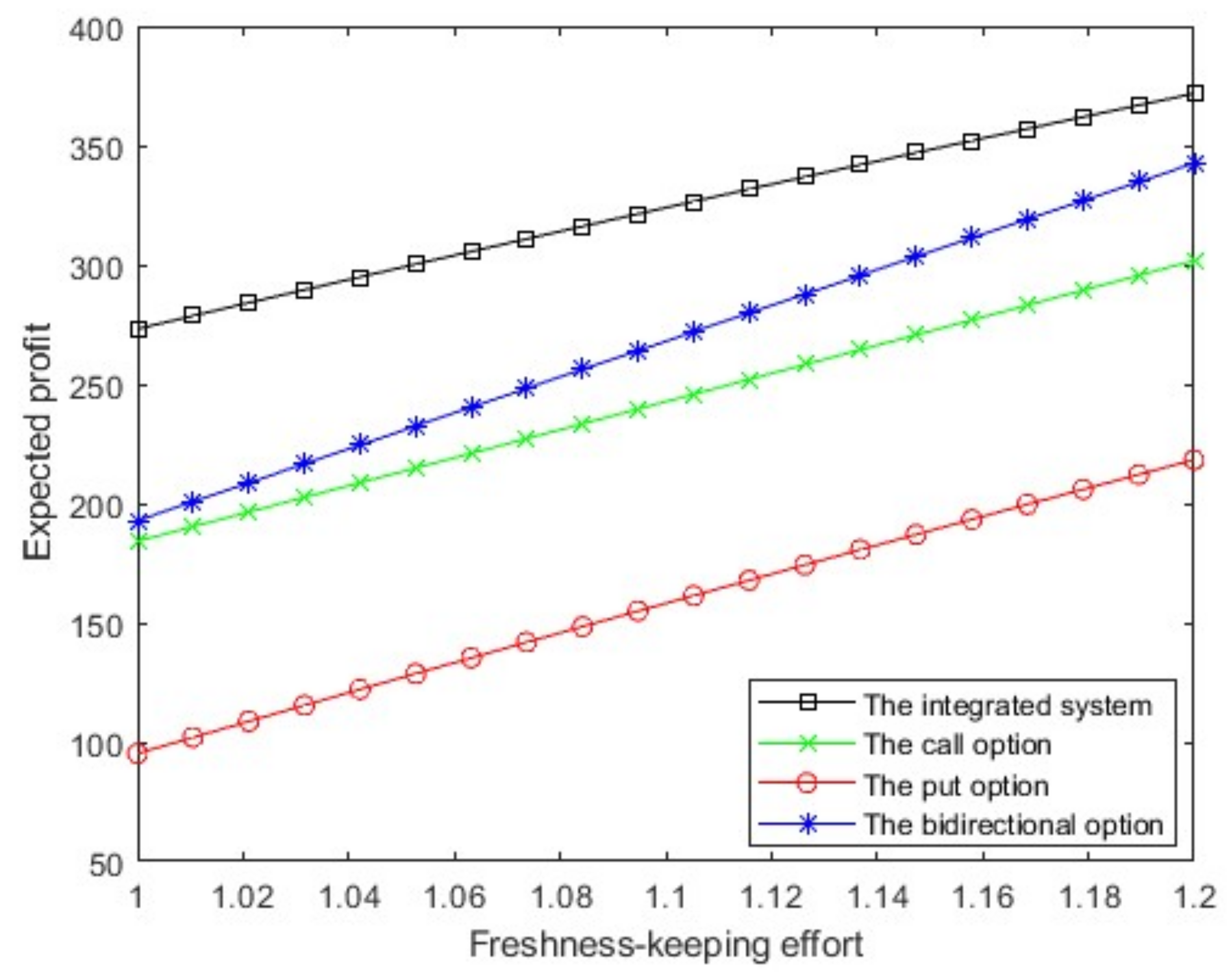
5.1. Comparison of Expected Profit
In this subsection, we set . Figure 1 illustrates the expected profit of the integrated supply chain and the expected profit of the retailer under the call, put and bidirectional option contracts in a decentralized supply chain. It can be seen that the expected profit increases with freshness-keeping effort. Figure 1 also shows that, among the three option contracts, the bidirectional option has the highest expected profit, since the retailer can either reorder or return products according to the actual demand. The expected profit under the call option is lower than that under the bidirectional option but higher than under the put option.

Figure 1.
Expected profit.
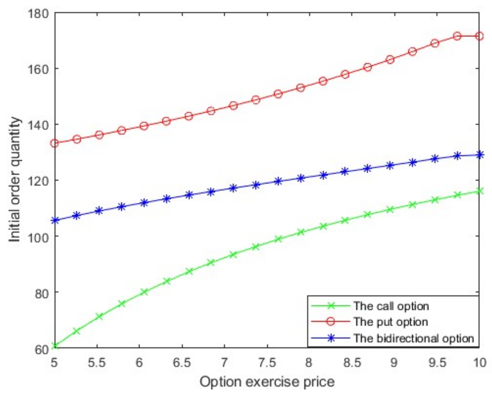
5.2. Comparison of Initial Order Quantities
Figure 2 shows the relationships between initial order quantity and option exercise price under the three option contracts; the results are consistent with Corollary 6. The put option contract has the highest initial order quantity because the retailer cannot reorder. Due to the option order cost of the bidirectional option contract being higher than those of the others, the retailer’s initial order quantity under the bidirectional option contract is higher than that under the call option contract.

Figure 2.
The initial order quantity.
The relationship between the option exercise price and the initial order quantity is also shown in Figure 2. The higher the option exercise price, the larger the initial order quantity; hence, there are positive correlations under all three contracts.
5.3. Comparison of Option Order Quantities
Figure 3 shows that the bidirectional option contract has the lowest option order quantity due to having the highest option price. With the same freshness-keeping effort and option exercise price, the option order quantities are equal under the call and put option contracts, which is consistent with Corollary 7. The option order quantity will decrease significantly as the option exercise price increases.
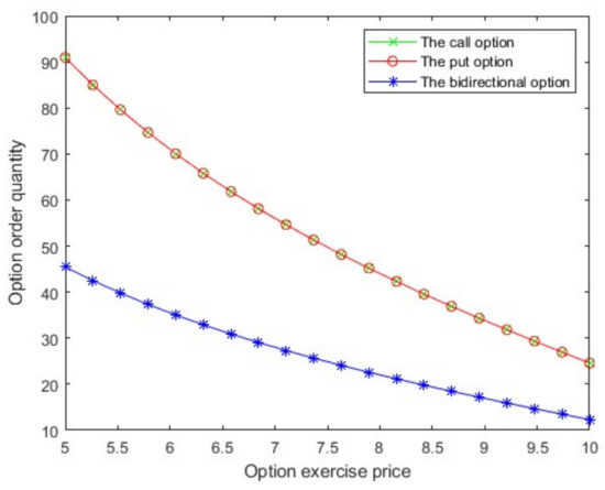
Figure 3.
The option order quantity.
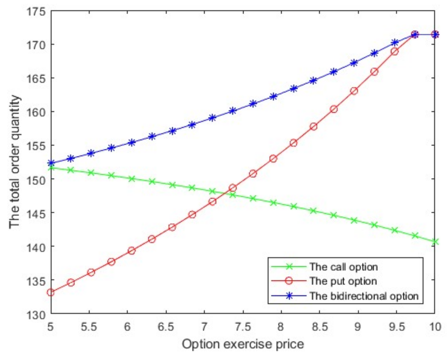
5.4. Comparison of Total Order Quantities
Figure 4 shows the retailer’s total order quantities in relation to the option exercise price under call, put and bidirectional option contracts; the results are consistent with Corollary 2, Corollary 3, and Corollary 4. It can be seen that under the put and bidirectional option contracts, the total order quantities increase with the option exercise price. Since the bidirectional option allows the reorder or return of fresh produce in the selling season, the total order quantity is higher than under the put option. As the option exercise price increases, the retailer’s willingness to order options will gradually decrease under the call option, resulting in the retailer’s total order quantity decreasing.

Figure 4.
The total order quantity.
6. Discussion and Conclusions
In this paper, we studied the retailer’s ordering decision and coordination strategy with freshness-keeping effort and option contracts. We developed the mathematical models of fresh produce supply chains considering the freshness-keeping effort and option contracts, and solved the following problems: (1) the retailer’s optimal ordering decision and freshness-keeping effort strategy under the wholesale price contract, call, put, and bidirectional option contracts are obtained; (2) the coordination conditions of the fresh produce supply chain considering option contracts and freshness-keeping effort are derived; and (3) the expected profits, initial order quantities, option order quantities and total order quantities of these three option contracts are compared.
Compared with previous studies, to our knowledge, we are the first that considered both freshness-keeping effort and option contract in the fresh produce supply chain. Our research shows that: (1) the retailer’s freshness-keeping effort can increase it’s expected profit; (2) option contracts can not only reduce the risks of overage and underage faced by retailers but also coordinate the fresh produce supply chain; and (3) the expected profit of a decentralized supply chain with option contracts is expected to be higher than that with a wholesale price contract. However, how the increased profit is distributed depends on the bargaining power of supply chain members.
Our research has important practical significance. As a special perishable product, fresh produce has the characteristics of long leading time, large circulation loss, no salvage value at the end of the selling season and requires high freshness, which makes the supply chain management of fresh produce face dramatic challenges. Therefore, our research has important practical significance for the retailer to reduce the risks of underage and overage in the supply chain, and to balance the relationship between freshness-keeping costs and profits. Furthermore, our finding has some theoretical significance. It applies option contracts to the fresh produce supply chain which provides a novel idea for risk management of supply chains.
Our study still has certain limitations, which can be our research directions in the future. Firstly, we did not consider the random yield of fresh produce, nor did we consider pricing strategy in relation to freshness-keeping effort. In real life, due to weather and natural disasters, yields are unpredictable and random. Thus, it is necessary to consider stochastic yield and to improve the application of option contracts in fresh produce supply chains. In addition, we assumed that both the supplier and retailer were risk-neutral; however, in reality, they may be risk-averse. Therefore, further research should consider the different risk preferences of supply chain members.
Author Contributions
Conceptualization, D.J. and C.W.; methodology, D.J. and C.W.; software, D.J. and C.W.; formal analysis, D.J. and C.W.; investigation, D.J. and C.W.; writing—original draft preparation, D.J.; writing—review and editing, C.W.; supervision, C.W.; funding acquisition, C.W. All authors have read and agreed to the published version of the manuscript.
Funding
This research is partly supported by the National Natural Science Foundation of China (No. 71972136), and Sichuan Science and Technology Program (No. 2022JDTD0022).
Institutional Review Board Statement
Not applicable.
Informed Consent Statement
Not applicable.
Acknowledgments
The authors would like to thank the editor and the anonymous reviewers for their valuable comments.
Conflicts of Interest
The authors declare that there are no conflicts of interest regarding the publication of this paper.
Appendix A
Appendix A.1. Proof of Proposition 1
Proof of Proposition 1.
In an integrated system, the expected profit function is as follows:
The expected profit function’s second-order partial derivative satisfies . Thus, the expected profit function is concave in . Let the expected profit function’s first-order partial derivative , so that the supplier’s optimal supply quantity is .
Given the optimal supply quantity , we can derive that . Thus, the expected profit function is concave in and the optimal freshness-keeping effort should satisfy . This completes the proof. □
Appendix A.2. Proof of Proposition 2
Proof of Proposition 2.
The expected profit function of the retailer under the wholesale price contract is as follows:
The second-order partial derivative of the expected profit of the retailer satisfies . So, the expected profit function of the retailer is concave in the order quantity under wholesale price contract. Let , therefore the optimal order quantity of the retailer is .
Given the optimal order quantity , we can derive that . Therefore, the retailer’s expected profit is concave in and the retailer’s optimal freshness-keeping effort under wholesale price contract should satisfy . This completes the proof. □
Appendix A.3. Proof of Corollary 1
Proof of Corollary 1.
The optimal freshness-keeping effort of the retailer should satisfy the following conditions in the integrated system and decentralized system respectively.
We have , so we can derive the . This completes the proof. □
Appendix A.4. Proof of Proposition 3
Proof of Proposition 3.
The expected profit function of the retailer with the call option contract is as follows:
, . , . And , , , it follows that the Hessian matrix of is negative definite. Thus, is jointly concave in and . Let , we obtain the optimal initial order quantity of the retailer under call option contract . Let , we can get the optimal total order quantity of the retailer under call option contract . Since , the retailer’s optimal option order quantity under call option contract is .
Given the optimal initial order quantity and optimal total ordering quantity , we can obtain that . Therefore, the expected profit of the retailer is concave in and optimal freshness-keeping effort of the retailer under the call option contract should satisfy . This completes the proof. □
Appendix A.5. Proof of Proposition 4
Proof of Proposition 4.
Combining Proposition 1 and Proposition 3, according to the coordination condition , , thus , then we get , i.e., . This completes the proof. □
Appendix A.6. Proof of Corollary 2
Proof of Corollary 2.
The optimal total order quantity of the retailer with the call option contract is , where . We can get . Let , we can get . We have . Thus, we have . According to Proposition 4, , we have . Therefore, we derive that decreases as increases. This completes the proof. □
Appendix A.7. Proof of Proposition 5
Proof of Proposition 5.
The expected profit function of the retailer with the put option contract is as follows:
, . , . , , , it follows that the Hessian matrix of is negative definite. Thus, is jointly concave in and . Let , we obtain the optimal initial order quantity of the retailer under the put option contract . Due to the characteristic of the put option contract, the optimal total order quantity of the retailer is equal to optimal initial order quantity. Thus, . Let , we can get the minimum expected sales quantity of the retailer under put option contract . Since , the optimal option order quantity of the retailer under put option contract is .
Given the and , we can obtain that . Therefore, the expected profit of the retailer is concave in and the optimal freshness-keeping effort of the retailer under the put option contract should satisfy the follow equation
.
This completes the proof. □
Appendix A.8. Proof of Proposition 6
Proof of Proposition 6.
The Proof of Proposition 6 is similar to the Proof of Proposition 4. □
Appendix A.9. Proof of Corollary 3
Proof of Corollary 3.
The optimal total order quantity of the retailer with the put option contract is , where . We can get . Let , we can get . We have . Thus, we have . According to Proposition 6, , we have . Therefore, we derive that increases as increases. This completes the proof. □
Appendix A.10. Proof of Proposition 7
Proof of Proposition 7.
The expected profit function of the retailer with the bidirectional option contract is as follows:
, . , . , , , it follows that the Hessian matrix of is negative definite. Thus, is jointly concave in and . Let , we obtain the retailer’s optimal total order quantity with the bidirectional option contract . Let , we can get the minimum expected sales quantity of the retailer under the bidirectional option contract . Since and , the optimal initial order quantity of the retailer under the bidirectional option contract is and the optimal option order quantity of the retailer with the bidirectional option contract is .
Given the and , we can derive that . Therefore, the expected profit of the retailer is concave in and the optimal freshness-keeping effort of the retailer under the bidirectional option contract should satisfy the follow equation
.
This completes the proof. □
Appendix A.11. Proof of Proposition 8
Proof of Proposition 8.
The proof of Proposition 8 is similar to the Proof of Proposition 4 and Proposition 6. □
Appendix A.12. Proof of Corollary 4
Proof of Corollary 4.
The optimal total order quantity of the retailer with the bidirectional option contract is , where . We can get . Let , we can get . We have . Thus, we have . According to Proposition 8, , we have . Therefore, we derive that increases as increases. This completes the proof. □
Appendix A.13. Proof of Corollary 5
Proof of Corollary 5.
Given and , we have that , , . Therefore, . Hence, we can get , . This completes the proof. □
Appendix A.14. Proof of Corollary 6
Proof of Corollary 6.
The optimal initial order quantity of the retailer under the bidirectional option contract is , , . Given , substitute into , we can get . Similarly, we have . So, . That is , . Substitute into , , so . That is and , . So, we have . Substitute into , . Since and . So and . This completes the proof. □
Appendix A.15. Proof of Corollary 7
Proof of Corollary 7.
With the call, put, and bidirectional option contract, the optimal option order quantity in a supply chain of fresh produce is , , , respectively. Given , substitute into , we can get . Substitute into , we obtain . Thus, the relationship between the optimal option order quantity in the fresh produce supply chain with the call, put and bidirectional option contract is as follows: . This completes the proof. □
References
- Wang, C.; Chen, X. Option pricing and coordination in the fresh produce supply chain with portfolio contracts. Ann. Oper. Res. 2016, 248, 471–491. [Google Scholar] [CrossRef]
- Wang, C.; Chen, X. Fresh produce price-setting newsvendor with bidirectional option contracts. J. Ind. Manag. Optim. 2021, 18, 1979–2000. [Google Scholar] [CrossRef]
- Xiao, Y.; Chen, J. Supply Chain Management of Fresh Products with Producer Transportation. Decis. Sci. 2012, 43, 785–815. [Google Scholar] [CrossRef]
- Cai, X.; Chen, J.; Xiao, Y.; Xu, X. Optimization and Coordination of Fresh Product Supply Chains with Freshness-Keeping Effort. Prod. Oper. Manag. 2010, 19, 261–278. [Google Scholar] [CrossRef]
- Wu, Q.; Mu, Y.; Feng, Y. Coordinating contracts for fresh product outsourcing logistics channels with power structures. Int. J. Prod. Econ. 2015, 160, 94–105. [Google Scholar] [CrossRef]
- Cachon, G.P.; Lariviere, M.A. Supply chain coordination with revenue-sharing contracts: Strengths and limitations. Manag. Sci. 2005, 51, 30–44. [Google Scholar] [CrossRef] [Green Version]
- Chen, X.; Hao, G.; Li, L. Channel coordination with a loss-averse retailer and option contracts. Int. J. Prod. Econ. 2014, 150, 52–57. [Google Scholar] [CrossRef]
- Wan, N.; Li, L.; Wu, X.; Fan, J. Coordination of a fresh agricultural product supply chain with option contract under cost and loss disruptions. PLoS ONE 2021, 16, e0252960. [Google Scholar] [CrossRef]
- Lee, C.-Y.; Li, X.; Xie, Y. Procurement risk management using capacitated option contracts with fixed ordering costs. IIE Trans. 2013, 45, 845–864. [Google Scholar] [CrossRef]
- Chen, X.; Shen, Z.-J. An analysis of a supply chain with options contracts and service requirements. IIE Trans. 2012, 44, 805–819. [Google Scholar] [CrossRef]
- Wang, C.; Chen, X. Optimal ordering policy for a price-setting newsvendor with option contracts under demand uncertainty. Int. J. Prod. Res. 2015, 53, 6279–6293. [Google Scholar] [CrossRef]
- Wang, C.; Chen, J.; Chen, X. Pricing and order decisions with option contracts in the presence of customer returns. Int. J. Prod. Econ. 2017, 193, 422–436. [Google Scholar] [CrossRef]
- Chen, F.; Parlar, M. Value of a put option to the risk-averse newsvendor. IIE Trans. 2007, 39, 481–500. [Google Scholar] [CrossRef]
- Chen, X.; Wan, N.; Wang, X. Flexibility and coordination in a supply chain with bidirectional option contracts and service requirement. Int. J. Prod. Econ. 2017, 193, 183–192. [Google Scholar] [CrossRef] [Green Version]
- Wang, C.; Chen, J.; Chen, X. The impact of customer returns and bidirectional option contract on refund price and order decisions. Eur. J. Oper. Res. 2019, 274, 267–279. [Google Scholar] [CrossRef]
- Yang, L.; Tang, R.; Chen, K. Call, put and bidirectional option contracts in agricultural supply chains with sales effort. Appl. Math. Model. 2017, 47, 1–16. [Google Scholar] [CrossRef]
- Blackburn, J.; Scudder, G. Supply Chain Strategies for Perishable Products: The Case of Fresh Produce. Prod. Oper. Manag. 2009, 18, 129–137. [Google Scholar] [CrossRef]
- Bai, R.; Burke, E.K.; Kendall, G. Heuristic, meta-heuristic and hyper-heuristic approaches for fresh produce inventory control and shelf space allocation. J. Oper. Res. Soc. 2008, 59, 1387–1397. [Google Scholar] [CrossRef]
- Qin, Y.; Wang, J.; Wei, C. Joint pricing and inventory control for fresh produce and foods with quality and physical quantity deteriorating simultaneously. Int. J. Prod. Econ. 2014, 152, 42–48. [Google Scholar] [CrossRef]
- Liu, G.; Zhang, J.; Tang, W. Joint dynamic pricing and investment strategy for perishable foods with price-quality dependent demand. Ann. Oper. Res. 2015, 226, 397–416. [Google Scholar] [CrossRef]
- He, B.; Gan, X.; Yuan, K. Entry of online presale of fresh produce: A competitive analysis. Eur. J. Oper. Res. 2019, 272, 339–351. [Google Scholar] [CrossRef]
- Yu, Y.; He, Y.; Zhao, X.; Zhou, L. Certify or not? An analysis of organic food supply chain with competing suppliers. Ann. Oper. Res. 2019, 1–31. [Google Scholar] [CrossRef]
- Chakraborty, D.; Garai, T.; Jana, D.K.; Roy, T.K. A three-layer supply chain inventory model for non-instantaneous deteriorating item with inflation and delay in payments in random fuzzy environment. J. Ind. Prod. Eng. 2017, 34, 407–424. [Google Scholar] [CrossRef]
- Garai, T.; Garg, H. Multi-objective linear fractional inventory model with possibility and necessity constraints under generalised intuitionistic fuzzy set environment. CAAI Trans. Intell. Technol. 2019, 4, 175–181. [Google Scholar] [CrossRef]
- Cai, X.; Chen, J.; Xiao, Y.; Xu, X.; Yu, G. Fresh-product supply chain management with logistics outsourcing. Omega 2013, 41, 752–765. [Google Scholar] [CrossRef]
- Yu, Y.; Xiao, T. Pricing and cold-chain service level decisions in a fresh agri-products supply chain with logistics outsourcing. Comput. Ind. Eng. 2017, 111, 56–66. [Google Scholar] [CrossRef]
- Song, Z.; He, S. Contract coordination of new fresh produce three-layer supply chain. Ind. Manag. Data Syst. 2019, 119, 148–169. [Google Scholar] [CrossRef]
- Mohammadi, H.; Ghazanfari, M.; Pishvaee, M.S.; Teimoury, E. Fresh-product supply chain coordination and waste reduction using a revenue-and-preservation-technology-investment-sharing contract: A real-life case study. J. Clean. Prod. 2019, 213, 262–282. [Google Scholar] [CrossRef]
- Zhao, Y.; Wang, S.; Cheng, T.C.E.; Yang, X.; Huang, Z. Coordination of supply chains by option contracts: A cooperative game theory approach. Eur. J. Oper. Res. 2010, 207, 668–675. [Google Scholar] [CrossRef]
- Fu, Q.; Zhou, S.X.; Chao, X.; Lee, C.-Y. Combined Pricing and Portfolio Option Procurement. Prod. Oper. Manag. 2012, 21, 361–377. [Google Scholar] [CrossRef] [Green Version]
- Luo, J.; Zhang, X.; Jiang, X. Multisources Risk Management in a Supply Chain under Option Contracts. Math. Probl. Eng. 2019, 2019, 1–12. [Google Scholar] [CrossRef]
- Gomez_Padilla, A.; Mishina, T. Supply contract with options. Int. J. Prod. Econ. 2009, 122, 312–318. [Google Scholar] [CrossRef]
- Xu, H. Managing production and procurement through option contracts in supply chains with random yield. Int. J. Prod. Econ. 2010, 126, 306–313. [Google Scholar] [CrossRef]
- Liang, L.; Wang, X.; Gao, J. An option contract pricing model of relief material supply chain. Omega 2012, 40, 594–600. [Google Scholar] [CrossRef]
- Nosoohi, I.; Nookabadi, A.S. Outsource planning with asymmetric supply cost information through a menu of option contracts. Int. Trans. Oper. Res. 2019, 26, 1422–1450. [Google Scholar] [CrossRef]
- Vafa Arani, H.; Rabbani, M.; Rafiei, H. A revenue-sharing option contract toward coordination of supply chains. Int. J. Prod. Econ. 2016, 178, 42–56. [Google Scholar] [CrossRef]
- Cai, J.; Zhong, M.; Shang, J.; Huang, W. Coordinating VMI supply chain under yield uncertainty: Option contract, subsidy contract, and replenishment tactic. Int. J. Prod. Econ. 2017, 185, 196–210. [Google Scholar] [CrossRef]
- Hu, B.; Qu, J.; Meng, C. Supply chain coordination under option contracts with joint pricing under price-dependent demand. Int. J. Prod. Econ. 2018, 205, 74–86. [Google Scholar] [CrossRef]
- Luo, J.; Chen, X. Risk hedging via option contracts in a random yield supply chain. Ann. Oper. Res. 2015, 257, 697–719. [Google Scholar] [CrossRef]
- Sharma, A.; Dwivedi, G.; Singh, A. Game-theoretic analysis of a two-echelon supply chain with option contract under fairness concerns. Comput. Ind. Eng. 2019, 137, 106096. [Google Scholar] [CrossRef]
- Biswas, I.; Avittathur, B. Channel coordination using options contract under simultaneous price and inventory competition. Transp. Res. Part E Logist. Transp. Rev. 2019, 123, 45–60. [Google Scholar] [CrossRef]
- Fan, Y.; Feng, Y.; Shou, Y. A risk-averse and buyer-led supply chain under option contract: CVaR minimization and channel coordination. Int. J. Prod. Econ. 2020, 219, 66–81. [Google Scholar] [CrossRef]
- Liu, Z.; Hua, S.; Zhai, X. Supply chain coordination with risk-averse retailer and option contract: Supplier-led vs. Retailer-led. Int. J. Prod. Econ. 2020, 223, 107518. [Google Scholar] [CrossRef]
- Jia, D.; Wang, C. Supply Chain Coordination of Loss-Averse Retailer for Fresh Produce with Option Contracts. In Proceedings of the LISS 2021, Jinan, China, 23–26 July 2021; pp. 1–10. [Google Scholar] [CrossRef]
- Xue, K.; Li, Y.; Zhen, X.; Wang, W. Managing the supply disruption risk: Option contract or order commitment contract? Ann. Oper. Res. 2018, 291, 985–1026. [Google Scholar] [CrossRef]
- Luo, J.; Zhang, X.; Wang, C. Using put option contracts in supply chains to manage demand and supply uncertainty. Ind. Manag. Data Syst. 2018, 118, 1477–1497. [Google Scholar] [CrossRef]
- Hu, Z.; Tian, J.; Feng, G. A relief supplies purchasing model based on a put option contract. Comput. Ind. Eng. 2019, 127, 253–262. [Google Scholar] [CrossRef]
- Wang, C.; Chen, J.; Wang, L.; Luo, J. Supply chain coordination with put option contracts and customer returns. J. Oper. Res. Soc. 2019, 71, 1003–1019. [Google Scholar] [CrossRef]
- Chen, X.; Luo, J.; Wang, X.; Yang, D. Supply chain risk management considering put options and service level constraints. Comput. Ind. Eng. 2020, 140, 106228. [Google Scholar] [CrossRef]
- Guo, P.; Jia, Y.; Gan, J.; Li, X. Optimal Pricing and Ordering Strategies with a Flexible Return Strategy under Uncertainty. Mathematics 2021, 9, 2097. [Google Scholar] [CrossRef]
- Bakhshi, A.; Heydari, J. An optimal put option contract for a reverse supply chain: Case of remanufacturing capacity uncertainty. Ann. Oper. Res. 2021, 1–24. [Google Scholar] [CrossRef]
- Zhao, Y.; Ma, L.; Xie, G.; Cheng, T.C.E. Coordination of supply chains with bidirectional option contracts. Eur. J. Oper. Res. 2013, 229, 375–381. [Google Scholar] [CrossRef]
- Luo, J.; Chen, X.; Wang, C.; Zhang, G. Bidirectional options in random yield supply chains with demand and spot price uncertainty. Ann. Oper. Res. 2021, 302, 211–230. [Google Scholar] [CrossRef]
- Wang, C.; Chen, X. Joint order and pricing decisions for fresh produce with put option contracts. J. Oper. Res. Soc. 2018, 69, 474–484. [Google Scholar] [CrossRef]
- Wan, N.; Chen, X. Contracts choice for supply chain under inflation. Int. Trans. Oper. Res. 2018, 25, 1907–1925. [Google Scholar] [CrossRef]
- Zhou, L.; Zhou, G.; Qi, F.; Li, H. Research on coordination mechanism for fresh agri-food supply chain with option contracts. Kybernetes 2019, 48, 1134–1156. [Google Scholar] [CrossRef]
- Chambers, C.; Kouvelis, P.; Semple, J. Quality-Based Competition, Profitability, and Variable Costs. Manag. Sci. 2006, 52, 1884–1895. [Google Scholar] [CrossRef] [Green Version]
- Liu, Z.; Anderson, T.D.; Cruz, J.M. Consumer environmental awareness and competition in two-stage supply chains. Eur. J. Oper. Res. 2012, 218, 602–613. [Google Scholar] [CrossRef]

Publisher’s Note: MDPI stays neutral with regard to jurisdictional claims in published maps and institutional affiliations. |
© 2022 by the author. Licensee MDPI, Basel, Switzerland. This article is an open access article distributed under the terms and conditions of the Creative Commons Attribution (CC BY) license (https://creativecommons.org/licenses/by/4.0/).