Robust Fuzzy Control for Uncertain Nonlinear Power Systems

Abstract

This paper presents a new control technique based on uncertain fuzzy models for handling uncertainties in nonlinear dynamic systems. This approach is applied for the stabilization of a multimachine power system subject to disturbances. In this case, a state-feedback controller based on parallel distributed compensation (PDC) is applied for the stabilization of the fuzzy system, where the design of control laws is based on the Lyapunov function method and the stability conditions are solved using a linear matrix inequalities (LMI)-based framework. Due to the high number of system nonlinearities, two steps are followed to reduce the number of fuzzy rules. Firstly, the power network is subdivided into sub-systems using Thevenin’s theorem. Actually, each sub-system corresponds to a generator which is in series with the Thevenin equivalent as seen from this generator. This means that the number of sub-systems is equal to the number of system generators. Secondly, the significances of the nonlinearities of the sub-systems are ranked based on their limits and range of variation. Then, nonlinearities with non-significant variations are assumed to be uncertainties. The proposed strategy is tested on the Western systems coordinating council (WSCC) integrated with a wind turbine. The disturbances are assumed to be sudden variations in wind power output. The effectiveness of the suggested fuzzy controller is compared with conventional regulators, such as an automatic voltage regulator (AVR) and power system stabilizers (PSS).

1. Introduction

Modeling a physical process aims to provide a mathematical description of its behavior at a particular point in space and/or time. Nevertheless, this description is mostly based on multiple assumptions, such as the insignificance of any delays and a lack of knowledge about some nonlinearities and non-stationary attitudes. These shortcomings often lead to inexactitudes and uncertainty of the parameters involved in the mathematical model of nonlinear systems, such as linearization coefficients whose values are often not sufficiently well known, change over time and depend on the operating conditions. Therefore, it is more reasonable to consider a set of models that encompasses uncertain elements instead of one model which is generally too restrictive. Recently, particular emphasis has been placed upon the utilization of fuzzy set theory to overcome the shortcomings of conventional modeling methods. As a matter of fact, fuzzy models have been introduced as promising models for describing uncertain nonlinear systems (UNSs) [1] where parametric uncertainties are approximated by fuzzy rules. Based on the fact that fuzzy set theory can solve annoyance problems in nonlinear system modeling, fuzzy models have been used for the design of feedback controllers for such systems. The Takagi-Sugeno fuzzy (TSF) model is one of the most widely used techniques for modeling and controlling nonlinear systems [2]. It is a universal approximation method consisting of a set of fuzzy IF-THEN rules which provides a linguistic description that is both transparent and interpretable by the user of the model. This representation can be constructed by integrating knowledge of the behavior of the system, given by experts, but also from the input–output data of the system, which provides a more systematic description of the model. The main feature of a TSF model is its ability to appropriately handle the uncertainties and nonlinearities of the systems to be controlled [2]. However, when it comes to complex systems with a large number of nonlinearities or input and output variables, the number of rules becomes prohibitive. Therefore, it is necessary to find a new reduced structure of IF–THEN rules, provided that it coincides as much as possible with the characteristics of the original model. Nonetheless, whichever the adopted fuzzy model, it is advised to test its performance on complex nonlinear systems. Notably, interconnected power networks are part thereof [2,3].

In recent years, the robust control of uncertain dynamical systems has aroused great interest among researchers due to the fact that, in practice, most systems are subject to uncertainties and disturbances [4]. In [5], a sliding-mode control (SMC) for a class of uncertain systems was proposed whereby a common sliding surface was designed using the weighted sum of the input matrices of sub-systems. Despite this approach being able to ensure asymptotical stability and facilitate system stability analyses, uncertainties were not considered in the control matrices. Moreover, it was assumed that disturbance bounds were known, which is certainly not always the case in practice. In order to enhance the dynamic performance of the SMC, a reaching law methodology was used in [6], in which fuzzy control was used to adjust its parameters. However, the number of fuzzy rules for large systems was not investigated. Moreover, SMC suffers from the chattering phenomenon in the control signal. Over the past two decades, adaptive control-based strategies have also been applied for various nonlinear systems in industry in such a way that the best possible controlled system operation is achieved, even if the system parameters are uncertain or time-varying [7,8,9]. Unfortunately, the design of an adaptive controller is based on various assumptions which are not always verified, and the performance of such controllers can be limited by significant levels of uncertainties [10].

To strengthen the dynamic performance of the adaptive control, various fuzzy-based adaptive control schemes have been developed without destroying the main basis on which adaptive control was built [11,12,13,14,15]. For instance, Boulkroune et al. [12] developed a fuzzy adaptive controller for UNS where the uncertain fuzzy parameters are online approximated by means of a proportional-integral adaptation procedure. The authors of [13] deployed fuzzy-based adaptive control for pure-feedback UNSs where fuzzy systems were adopted to estimate the uncertainties. Generally speaking, Lyapunov’s theory has been employed to establish the parametric adaptation law and analyze the stability of adaptive controllers. However, the principal drawbacks of these control schemes were examined, either by using simple simulations or adopting particular cases. It was found that their robustness and effectiveness for real-world cases could be determined. In [16], another outstanding approach, called time delay control (TDC), was presented for the robust control of a class of UNSs whereby an approach based on the Lyapunov-Krasvoskii method was established for stability analyses of the TDC. Unfortunately, only a simple test case was investigated. Moreover, the design of the TDC requires appropriate knowledge of all the system states as well as their derivatives, which is not usually available in practice.

Other type of controller scheme based on a state-feedback controller was developed in [17,18] where the TSF was employed to model nonlinear systems to be controlled, and parallel distributed compensation (PDC) -based controllers were successfully applied for the stabilization of the systems. Generally speaking, the PDC approach is based on linear controllers designed for each of the interconnected linear models, and the closed-loop stability of the assembly is ensured through a Lyapunov function common to all the sub-models [17]. On the basis of a literature review, it was found that the stability conditions of the TSF models are frequently solved using linear matrix inequalities (LMIs) based frameworks [18]. Although the choice of the test system is one of the most important parameters for testing any controller, it has been a point of weakness for some controllers. Power system stability is one among a number of illustrative examples which has been used to evaluate the performance of fuzzy-based controllers [19,20,21]. For instance, the authors of [20] presented a fuzzy logic-based power system stabilizer (PSS) to enhance power system stability, where the fuzzy rules were elaborated using a trial and error approach. Unfortunately, the reduction of the number of rules for large power networks was not discussed. Ansari et al. [21] developed optimal coordination between a fuzzy controller based static compensator (STATCOM) and fuzzy PSS for damping low frequency oscillations, where 17 out of 49 rules were related to seven fuzzy sets.

In this paper, a new fuzzy controller for UNS is developed and applied for an uncertain multimachine power system. A strategy based on the approach developed in [22] is used to describe the UNS by the TSF models. Unfortunately, that reference did not discuss the large number of fuzzy rules, especially when dealing with complex nonlinear systems having significant numbers of nonlinearities. The stabilization of the fuzzy system is achieved by performing linear state feedback. This is supplanted by a PDC controller law which takes into account the nonlinearities of the fuzzy models. The principle of this controller consists of designing a state-feedback controller for each local model. The global control law is obtained by the interpolation of the local linear control laws. Therefore, the main contributions of this paper are as follows:

• In order to overcome the complexities of power grids, a novel strategy for modeling a multimachine power system by TSF is developed. In this strategy, a multimachine system is subdivided into sub-systems equivalent to single machine infinite bus (SMIB) systems. Each sub-system corresponds to a generating unit in series with the Thevenin equivalent seen from this unit. The rest of the multimachine network, as seen from each machine, is therefore considered as a Thevenin model composed of a voltage source V_th in series with resistance R_th and reactance X_th. The Thevenin equivalent parameters are calculated after solving the load flow problem under various operating conditions. As a result, no assumptions are made, which leads to accurate modeling of the studied system. It should be noted that the number of these sub-systems is equal to the number of system machines. The complete model of each SMIB system is determined based on Blondel’s diagram [23]. To the best of the authors’ knowledge, this strategy has not been applied in other published works.
• In order to represent SMIB systems using TSF models, each nonlinearity is described by two fuzzy rules. It is worth noting that each SMIB system model has four nonlinearities, which results in 16 fuzzy rules for each sub-system; therefore, the greater the number of generators, the greater the number of fuzzy rules. Thus, a new method for reducing the number of fuzzy rules is presented in this study. In this method, the significances of the nonlinearities of sub-systems are ranked based on their limits and variation range under various operating conditions. Then, nonlinearities with non-significant variations are assumed to be uncertainties. This might be useful in applying the proposed uncertain fuzzy controller (UFC) in a more efficient and effective way. In this study, the parameters of the UFC laws are tuned using the Lyapunov function method, where the stability conditions are solved using an LMI-based framework.
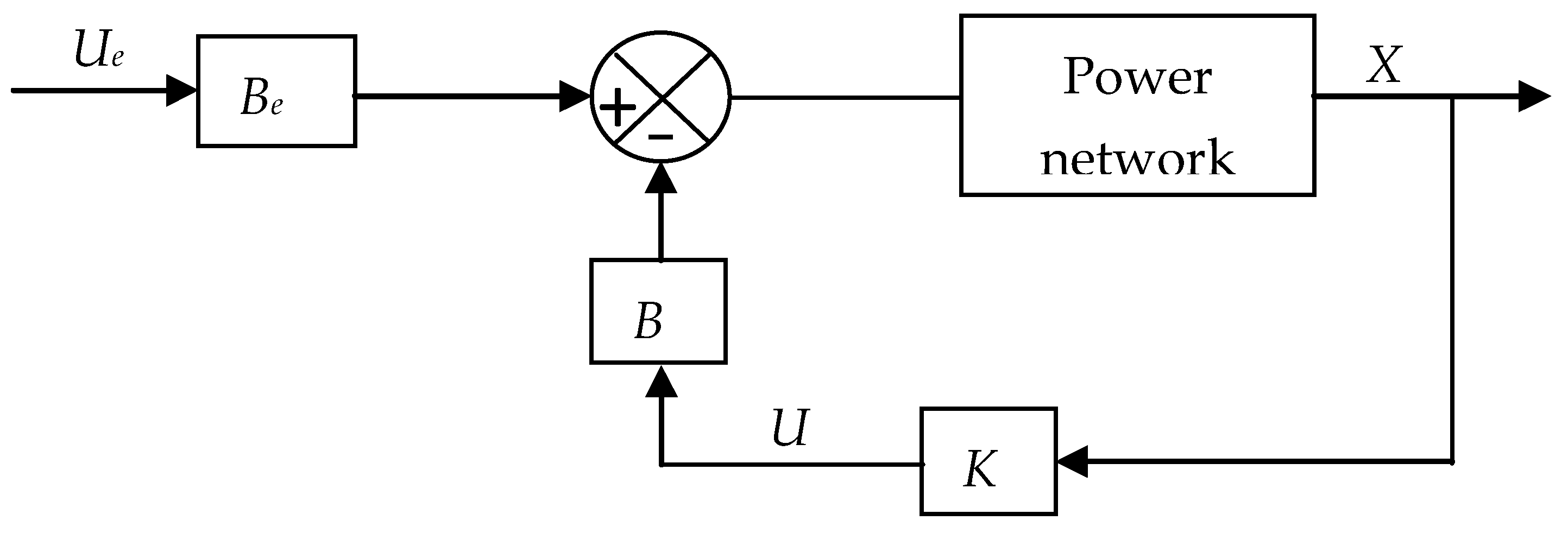
• The applicability and robustness of the proposed UFC are tested for the stabilization of a multimachine power system. The controller is applied directly to the PSS regulators, aiming to increase the damping of system oscillations after the occurrence of disturbances. To the best of our knowledge, this is the first attempt to apply the proposed UFC to the stabilization of a multimachine power system. According to our simulation results, the proposed controller achieved an accurate representation of the system and responded effectively to changes in the system operating conditions.

This research paper is organized as follows: In Section 2, a detailed description of the fuzzy Takagi-Sugeno model is presented. In Section 3, the LMI conditions for the stabilization of an uncertain fuzzy system are developed. Then, the stabilization of an uncertain fuzzy system based on decay rate is presented in Section 4. The modeling of a multimachine power system by TSF is presented in Section 5. Numerical simulations to test the robustness and applicability of the proposed controller are presented in Section 6. Finally, Section 7 gives the main conclusions.

2. Proposed TSF Modeling Method for Nonlinear Systems

In this study, a new technique based on the approach developed in [22] is used to describe nonlinear systems by TSF models. In that approach, each nonlinearity of the nonlinear system to be modeled is described by two fuzzy sub-systems defined by their minimum and maximum bounds. Thus, the proposed technique can be summarized as follows.

Let us consider a nonlinear system having one nonlinearity described by its state-space equation, as given in Equation (1).

$$\dot{X}=\left(\begin{array}{cc}a& N\left(X\right)\\ b& c\end{array}\right)X+BU$$

(1)

where X is the state vector, U is the input vector, B is the input matrix, $\left(\begin{array}{cc}a& N\left(X\right)\\ b& c\end{array}\right)$ is the state matrix and $N\left(X\right)$ is the system nonlinearity, which can be rewritten as follows:

$$N\left(X\right)=\frac{M-N\left(X\right)}{M-m}m+\frac{N\left(X\right)-m}{M-m}M=h_1\left(X\right)m+h_2\left(X\right)M$$

(2)

where m and M are the lower and upper bounds of $N\left(X\right)$, $h_1=\frac{M-N\left(X\right)}{M-m}$ and $h_2=\frac{N\left(X\right)-m}{M-m}$. It is worth noting that $0\le h_1\le 1$, $0\le h_2\le 1$ and $h_1+h_2=1$.

By substituting (2) into (1):

$$\dot{X}=\left(\begin{array}{cc}a& h_1\left(X\right)m+h_2\left(X\right)M\\ b& c\end{array}\right)X+BU$$

(3)

However, $\forall G$, $h_{1}G+h_{2}G=G$. Thus

$$\dot{X}=h_1\left(\begin{array}{cc}a& m\\ b& c\end{array}\right)X+h_2\left(\begin{array}{cc}a& M\\ b& c\end{array}\right)X+BU$$

(4)

Equation (4) can be rewritten as follows:

$$\dot{X}=(h_1{A}_1+h_2{A}_2)X+BU$$

(5)

where $A_1=\left(\begin{array}{cc}a& m\\ b& c\end{array}\right)$ and $A_2=\left(\begin{array}{cc}a& M\\ b& c\end{array}\right)$. $h_1$ and $h_2$ are the attribute weights for the fuzzy subsets.

The above description can be generalized for the case when the system contains two nonlinearities, i.e., $N_1\left(X\right)$ and $N_2\left(X\right)$, as shown in Equation (6). Thus, that system can be described by the interconnection of the local sub-systems, as given in Equation (7)

$$\dot{X}=\left(\begin{array}{cc}a& N_1\left(X\right)\\ N_2\left(X\right)& d\end{array}\right)X+BU$$

(6)

$$\dot{X}={\displaystyle \sum }_{i=1}^{i=4}{h}_i\left(X\right)A_{i}X+BU$$

(7)

where

$$\{\begin{array}{c}{A}_1=\left(\begin{array}{cc}a& m_1\\ m_2& d\end{array}\right)\mathrm{and} h_1\left(X\right)=F_{m1}{F}_{m2}\\ A_2=\left(\begin{array}{cc}a& m_1\\ M_2& d\end{array}\right)\mathrm{and} h_2\left(X\right)=F_{m1}{F}_{M2}\\ A_3=\left(\begin{array}{cc}a& M_1\\ m_2& d\end{array}\right)\mathrm{and} h_3\left(X\right)=F_{M1}{F}_{m2}\\ A_4=\left(\begin{array}{cc}a& M_1\\ M_2& d\end{array}\right)\mathrm{and} h_4\left(X\right)=F_{M1}{F}_{M2}\end{array}$$

(8)

In Equation (8), $F_{mi}=\frac{M_i-N_i\left(X\right)}{M_i-m_i}$ and $F_{Mi}=\frac{N_i\left(X\right)-m_i}{M_i-m_i}$ for $i\in \left\{0,1\right\}$.

Remarks 1.

It is worth noting that:

• if n is the number of nonlinearities, then the number of the local sub-systems is $2^n$ and the number of fuzzy rules is also $2^n$;
• if some nonlinearities are the same or proportional, then only one nonlinearity among them will be considered.

3. Stabilization of an Uncertain Fuzzy System

An UNS can be governed by a fuzzy system with uncertainties, and therefore, can be expressed by the following equation. In Equation (9), N denotes the number of fuzzy rules, i.e., $N=2^n$.

$$\{\begin{array}{c}\dot{X}={\displaystyle {\displaystyle \sum }_{i=1}^{i=N}}{h}_i\left[(A_i+\Delta A_i)X+(B_i+\Delta B_i)U\right]\\ Y={\displaystyle {\displaystyle \sum }_{i=1}^{i=N}}{h}_i(C_i+\Delta C_i)X\end{array}$$

(9)

Or

$$\{\begin{array}{c}\dot{X}=(A_h+\Delta A_h)X+(B_h+\Delta B_h)U\\ Y=(C_h+\Delta C_h)X\end{array}$$

(10)

Note that any notation in the form of $Z_h$ represents the following expression.

$$Z_h={\displaystyle \sum }_{i=1}^{i=N}{h}_i{Z}_i$$

(11)

For example, $A_h={\displaystyle \sum }_{i=1}^{i=N}{h}_i{A}_i$, $B_h={\displaystyle \sum }_{i=1}^{i=N}{h}_i{B}_i$ and so on.

$\Delta A_i$, $\Delta B_i$ and $\Delta C_i$ are bounded matrices which represent the parametric uncertainties in the following forms:

$$\{\begin{array}{c}\Delta A_i=H_{a_i}\Delta a_i{E}_{a_i}\\ \Delta B_i=H_{b_i}\Delta b_i{E}_{b_i}\\ \Delta C_i=H_{c_i}\Delta c_i{E}_{c_i}\end{array}$$

(12)

where $H_{a_i}$, $H_{b_i}$, $H_{c_i}$, $E_{a_i}$, $E_{b_i}$ and $E_{c_i}$ are known real constant matrices. $\Delta a_i$, $\Delta b_i$ and $\Delta c_i$ are bounded unknown matrix functions which verify the following conditions:

$$\{\begin{array}{c}\Delta a_i^T\Delta a_i\le I\\ \Delta b_i^T\Delta b_i\le I\\ \Delta c_i^T\Delta c_i\le I\end{array}$$

(13)

where I is the identity matrix.

The closed-loop model of Equation (9), when a PDC control law in the form of $U=-K_{h}X$ is applied, is expressed by Equation (14). Similarly to Equation (11), $K_h$ can be written in the following form.

$$K_h={\displaystyle \sum }_{i=1}^{i=N}{h}_i{K}_i$$

$$\dot{X}={\displaystyle \sum }_{i=1}^{i=N}{\displaystyle \sum }_{j=1}^{j=N}{h}_i{h}_j\left(A_i+\Delta A_i-(B_i+\Delta B_i)K_j\right)X$$

(14)

In most cases, the design of fuzzy controllers based on PDC has involved the application of the quadratic Lyapunov function. Generally speaking, the stability conditions are expected to be expressed as the LMI framework.

Let us consider a quadratic Lyapunov function $V\left(X\right)=X^{T}PX$, where P is a positive definite symmetric matrix. Therefore, the fuzzy system is asymptotically stable if the inequalities given in Equations (15) and (16) are verified, i.e., ∀$i=1, 2, \dots , r \mathrm{and} i<j\le r$.

$${\left(A_i+\Delta A_i-(B_i+\Delta B_i)K_i\right)}^{T}P+P\left(A_i+\Delta A_i-(B_i+\Delta B_i)K_i\right)<0$$

(15)

$$\begin{gathered} {\left(A_i+\Delta A_i-(B_i+\Delta B_i)K_j\right)}^{T}P+P\left(A_i+\Delta A_i-(B_i+\Delta B_i)K_j\right)+{\left(A_j+\Delta A_j-(B_j+\Delta B_j)K_i\right)}^{T}P \\ +P\left(A_j+\Delta A_j-(B_j+\Delta B_j)K_i\right)<0 \end{gathered}$$

(16)

Inequalities (15) and (16) can be rearranged as LMI conditions. With this aim, let us consider $L=P^{-1}$ and $M_i=K_{i}L$. Thus, inequality (15) is as follows:

$$L{A}_i^T+A_{i}L-M_i^T{B}_i^T-B_i{M}_i+L\Delta A_i^T+\Delta A_{i}L-M_i^T\Delta B_i^T-\Delta B_i{M}_i<0$$

(17)

By substituting (12) into (17), then

$$L{A}_i^T+A_{i}L-M_i^T{B}_i^T-B_i{M}_i+L{E}_{a_i}^T\Delta a_i^T{H}_{a_i}^T+H_{a_i}\Delta a_i{E}_{a_i}L-M_i^T{E}_{b_i}^T\Delta b_i^T{H}_{b_i}^T-H_{b_i}\Delta b_i{E}_{b_i}{M}_i<0$$

(18)

Before proceeding, the following two lemmas derived from [24] are recalled.

Lemma 1.

Let us consider a scalar$\epsilon >0$and two matrices V and W. Then

$$V^{T}W+W^{T}V\le \epsilon V^{T}V+{\epsilon }^{-1}{W}^{T}W$$

(19)

Lemma 2 (Schur complement).

Let us consider three matrices$Q=Q^T$, $R=R^T$and S. Then, the following three conditions are equivalent.

$$\left\{\left(\begin{array}{cc}Q& S\\ S^T& R\end{array}\right)>0\right\}\iff \left\{Q-S{R}^{-1}{S}^T>0\mathrm{and}R>0\right\} \iff \left\{R-S^T{Q}^{-1}S>0\mathrm{and}Q>0\right\}$$

(20)

Therefore, by using Equation (13), inequality (18) can be converted into LMI form as given by Equation (21). The same applies to Equation (16), where the LMI condition given by Equation (22) can be obtained.

$$\left[\begin{array}{ccc}L{A}_i^T+A_{i}L-M_i^T{B}_i^T-B_i{M}_i+{\epsilon }_{a_{ii}}{H}_{a_i}{H}_{a_i}^T+{\epsilon }_{b_{ii}}{H}_{b_i}{H}_{b_i}^T& L{E}_{a_i}^T& M_i^T{E}_{b_i}^T\\ E_{a_i}L& -{\epsilon }_{a_{ii}}I& 0\\ E_{b_i}{M}_i& 0& -{\epsilon }_{b_{ii}}I\end{array}\right]<0$$

(21)

$$\begin{gathered} \left[\begin{array}{ccc}L{A}_i^T+A_{i}L-M_j^T{B}_i^T-B_i{M}_j+{\epsilon }_{a_{ij}}{H}_{a_i}{H}_{a_i}^T+{\epsilon }_{b_{ij}}{H}_{b_i}{H}_{b_i}^T& L{E}_{a_i}^T& M_j^T{E}_{b_i}^T\\ E_{a_i}L& -{\epsilon }_{a_{ij}}I& 0\\ E_{b_i}{M}_j& 0& -{\epsilon }_{b_{ij}}I\end{array}\right]+ \\ \left[\begin{array}{ccc}L{A}_j^T+A_{j}L-M_i^T{B}_j^T-B_j{M}_i+{\epsilon }_{a_{ji}}{H}_{a_j}{H}_{a_j}^T+{\epsilon }_{b_{ji}}{H}_{b_j}{H}_{b_j}^T& L{E}_{a_j}^T& M_i^T{E}_{b_j}^T\\ E_{a_j}L& -{\epsilon }_{a_{ji}}I& 0\\ E_{b_j}{M}_i& 0& -{\epsilon }_{b_{ji}}I\end{array}\right]<0 \end{gathered}$$

(22)

4. Stabilization of Uncertain Fuzzy System Based on Decay Rate

The decay rate makes it possible to act on the dynamics (poles) of closed-loop sub-models; this consists of imposing a decay rate denoted by α on the decay of the Lyapunov function [25]. Thus, the stability condition is as follows:

$$\dot{V}\left(X\right)<-2\alpha V\left(X\right)$$

(23)

Knowing that

$$\dot{X}=\left(A_h+\Delta A_h-(B_h+\Delta B_h)K_h\right)X$$

(24)

Thus

$$\dot{V}\left(X\right)={\dot{X}}^{T}PX+X^{T}P\dot{X}=X^T\left[{\left(A_h+\Delta A_h-(B_h+\Delta B_h)K_h\right)}^{T}P+P\left(A_h+\Delta A_h-(B_h+\Delta B_h)K_h\right)\right]X$$

(25)

From (23) and (25), it follows that

$${\left(A_h+\Delta A_h-(B_h+\Delta B_h)K_h\right)}^{T}P+P\left(A_h+\Delta A_h-(B_h+\Delta B_h)K_h\right)+2\alpha P<0$$

(26)

After congruence by $P^{-1}=L$, inequality (26) becomes

$$L{\left(A_h+\Delta A_h-(B_h+\Delta B_h)K_h\right)}^T+\left(A_h+\Delta A_h-(B_h+\Delta B_h)K_h\right)L+2\alpha L<0$$

which means that

$$L{A}_h^T+A_{h}L+L\Delta A_h^T+\Delta A_{h}L-M_h^T{B}_h^T-B_h{M}_h-M_h^T\Delta B_h^T-\Delta B_h{M}_h+2\alpha L<0$$

(27)

where

$$M_h=K_{h}L$$

(28)

Replacing $\Delta A_{h}by{H}_{a_h}\Delta a_h{E}_{a_h}and\Delta B_{h}by{H}_{b_h}\Delta b_h{E}_{b_h}$ yields

$$L{A}_h^T+A_{h}L-M_h^T{B}_h^T-B_h{M}_h+L{E}_{a_h}^T\Delta a_h^T{H}_{a_h}^T+H_{a_h}\Delta a_h{E}_{a_h}L-M_h^T{E}_{b_h}^T\Delta b_h^T{H}_{b_h}^T-H_{b_h}\Delta b_h{E}_{b_h}{M}_h+2\alpha L<0$$

(29)

Applying Lemma 1, inequality (29) becomes

$$L{A}_h^T+A_{h}L-M_h^T{B}_h^T-B_h{M}_h+{\epsilon }_{a_h}{H}_{a_h}{H}_{a_h}^T+{\epsilon }_{a_h}^{-1}L{E}_{a_h}^T{E}_{a_h}L+{\epsilon }_{b_h}{H}_{b_h}{H}_{b_h}^T+{\epsilon }_{b_h}^{-1}{M}_h^T{E}_{b_h}^T{E}_{b_h}{M}_h+2\alpha L<0$$

(30)

Lemma 3.

Let A and Q be two matrices of appropriate dimensions, and P a positive definite symmetric matrix ($P>0$). Properties Pr 1 and Pr 2 are equivalent.

• Pr 1:$A^{T}PA-Q<0$
• Pr 2:$\exists X \mathit{and} Y$such that$\left(\begin{array}{cc}-Q{A}^T{Y}^T+YA& -Y+A^{T}X\\ -Y^T+X^{T}A& P-X-X^T\end{array}\right)<0$

Lemma 4.

Let A and Q be two matrices of appropriate dimensions, and P a positive definite symmetric matrix ($P>0$). Properties Pr 1 and Pr 2 are equivalent.

• Pr 1:$P{A}^T+AP-Q<0$
• Pr 2:$\exists X \mathit{and} Y$such that:$\left(\begin{array}{cc}X{A}^T+A{X}^T-Q& P-X+AY\\ P-X^T+Y^T{A}^T & -Y-Y^T\end{array}\right)<0$

Applying Lemmas 3 and 4 and employing the Schur’s complement yields the following LMI:

$$G_{hh}<0$$

(31)

where

$$G_{hh}=\left[\begin{array}{cccccc}{X}_{hh}& Y_{hh}^T& L{E}_{a_h}^T& -{\Phi }_{b_h}+H_{b_h}{\Psi }_{b_h}& M_h^T{E}_{b_h}^T& L-{\Theta }_h+A_h{\Sigma }_h\\ Y_{hh}& Z_{a_h}& 0& 0& 0& 0\\ E_{a_h}L& 0& -{\epsilon }_{a_h}I& 0& 0& 0\\ -{\Phi }_{b_h}^T+{\Psi }_{b_h}^T{H}_{b_h}^T& 0& 0& Z_{b_h}& 0& 0\\ E_{b_h}{M}_h& 0& 0& 0& -{\epsilon }_{b_h}I& 0\\ L-{\Theta }_h^T+{\Sigma }_h^T{A}_h^T& 0& 0& 0& 0& -{\Sigma }_h-{\Sigma }_h^T\end{array}\right]$$

(32)

with

$$X_{hh}=H_{a_h}{\Phi }_{a_h}^T+{\Phi }_{a_h}{H}_{a_h}^T+H_{b_h}{\Phi }_{b_h}^T+{\Phi }_{b_h}{H}_{b_h}^T-B_h{M}_h-M_h^T{B}_h^T+{\Phi }_h{A}_h^T+A_h{\Phi }_h^T+2\alpha L$$

(33)

$$Y_{hh}=-{\Phi }_{a_h}^T+{\Psi }_{a_h}^T{H}_{a_h}^T$$

(34)

$$Z_{a_h}={\epsilon }_{a_h}I-{\Psi }_{a_h}-{\Psi }_{a_h}^T$$

(35)

$$Z_{b_h}={\epsilon }_{b_h}I-{\Psi }_{b_h}-{\Psi }_{b_h}^T$$

(36)

5. Power System Modeling

Generally, a power network contains electrical machines with excitation systems, loads connected at the system buses and transmission lines.

5.1. Subdivision of a Power System into SMIB Sub-Systems

In order to apply decentralized control, it would be better to transform the power system with N_g synchronous machines to N_g sub-systems. Each sub-system is composed of one generator (G) connected to the rest of the network. The rest of the network is the Thevenin equivalent, as seen from this generator. The equivalent circuit of such a sub-system is shown in Figure 1. This circuit is equivalent to a single machine connected to an infinite bus.

R_Th, X_Th and V_Th shown in Figure 1 depend on the generated powers P_T and Q_T, total load and the network topology.

5.2. Calculation of the Parameters of the Thevenin Equivalent Circuit

Let us consider ${\overline{I}}_g$ the vector of the generator currents. ${\overline{I}}_g$ can be expressed as follows:

$${\overline{I}}_g={\overline{Y}}_p{\overline{V}}_T$$

(37)

where ${\overline{Y}}_p$ is the reduced admittance matrix which has the dimension (N_g × N_g), and ${\overline{V}}_T$ is the vector of generator voltages.

The real and reactive powers injected by the i-th generator can be calculated using Equations (38) and (39), respectively.

$$P_{Ti}={{\displaystyle \sum }}_{j=1}^{N_g}{V}_{Ti}{V}_{Tj}{Y}_{pij}cos\left({\alpha }_i-{\alpha }_j-{\theta }_{ij}\right)$$

(38)

$$Q_{Ti}={{\displaystyle \sum }}_{j=1}^{N_g}{V}_{Ti}{V}_{Tj}{Y}_{pij}sin\left({\alpha }_i-{\alpha }_j-{\theta }_{ij}\right)$$

(39)

where $V_{Ti}$ and ${\alpha }_i$ are the magnitude and phase angle of the i-th element of ${\overline{V}}_T$. $Y_{pij}$ and ${\theta }_{ij}$ are the magnitude and angle of ij-th element of ${\overline{Y}}_p$.

Let us consider

$${\overline{Z}}_p={\overline{Y}}_p^{-1}$$

(40)

$${\overline{V}}_{Ti}(1-{\displaystyle \sum }_{j\ne i}^{N_g}{\overline{Z}}_{pij}{\overline{Y}}_{pji})={\overline{Z}}_{pii}{\overline{I}}_{gi}+{\displaystyle \sum }_{j\ne i}^{N_g}\left({\overline{Z}}_{pij}\times {\displaystyle \sum }_{k\ne i}^{N_g}{\overline{Y}}_{pjk}{\overline{V}}_{Tk}\right)$$

where ${\overline{Z}}_{pij}$ is the ij-th element of ${\overline{Z}}_p$ and ${\overline{I}}_{gi}$ is the i-th element of ${\overline{I}}_g$.

Therefore, the terminal voltage ${\overline{V}}_{Ti}$ of the i-th generator can be expressed by the following equation:

$${\overline{V}}_{Ti}={\overline{Z}}_{Thi}{\overline{I}}_{gi}+{\overline{V}}_{Thi}$$

(41)

where

$${\overline{Z}}_{Thi}=\frac{{\overline{Z}}_{pii}}{1-{{\displaystyle \sum }}_{j\ne i}^{N_g}{\overline{Z}}_{pij}{\overline{Y}}_{pji}}=R_{Thi}+j{X}_{Thi}$$

(42)

$${\overline{V}}_{Thi}=\frac{{{\displaystyle \sum }}_{j\ne i}^{N_g}\left({\overline{Z}}_{pij}\times {{\displaystyle \sum }}_{k\ne i}^{N_g}{\overline{Y}}_{pjk}{\overline{V}}_{Tk}\right)}{1-{{\displaystyle \sum }}_{j\ne i}^{N_g}{\overline{Z}}_{pij}{\overline{Y}}_{pji}}$$

(43)

where R_Thi, X_Thi and V_Thi are the Thevenin equivalent circuit parameters of the i-th sub-system.

5.3. Dynamic Model of a Synchronous Machine

For a stability analysis, synchronous machines are often modeled by the third-order model. The set of nonlinear differential-algebraic equations describing that model [26] are given in Equations (44)–(46).

$$\frac{d\delta }{dt}=\omega$$

(44)

$$\frac{d\omega }{dt}=\frac{1}{2H}\left(P_m-P_e-K_D\omega \right)$$

(45)

$$\frac{d{E}_q^{\prime }}{dt}=\frac{1}{T_{d0}^{\prime }}(E_{fd}-E_q^{\prime }-\left(X_d-X_d^{\prime }\right)I_d)$$

(46)

where $\delta$ and $\omega$ are the rotor angle and rotor speed of the generator, respectively; $P_m$ and $P_e$ are the input and output power of the machine, respectively; $E_{fd}$ and $E_q^{\prime }$ are the field and internal voltages, respectively; $I_d$ is the d-axis armature current; and H, $K_D$, $T_{d0}^{\prime }$, $X_d$ and $X_d^{\prime }$ are the inertia constant, damping coefficient, transient time constant, d-axis reactance and d-axis transient reactance of the synchronous machine, respectively.

A Blondel diagram of a synchronous machine connected to the rest of a network, modeled by its Thevenin equivalent, is shown in Figure 2.

From the Blondel diagram in Figure 2, the following expressions can be deduced.

$$P_e=E_q{I}_q+E_d{I}_d$$

(47)

$$E_q=E_q^{\prime }+\left(X_d-X_d^{\prime }\right)I_d$$

(48)

$$I_d=\frac{1}{R_x^{\prime }}(X_{qs}{E}_q^{\prime }-X_{qs}{V}_{Th}\cos \left(\delta \right)-R_{Th}{V}_{Th}\sin \left(\delta \right))$$

(49)

$$I_q=\frac{1}{R_x^{\prime }}(R_{Th}{E}_q^{\prime }-R_{Th}{V}_{Th}\cos \left(\delta \right)+X_{ds}^{\prime }{V}_{Th}\sin \left(\delta \right))$$

(50)

where

$$X_{qs}=X_q+X_{Th}$$

(51)

$$X_{ds}^{\prime }=X_d^{\prime }+X_{Th}$$

(52)

$$X_{ds}=X_d+X_{Th}$$

(53)

$$R_x^{\prime }=R_{Th}^2+X_{ds}^{\prime }{X}_{qs}$$

(54)

$$R_x=R_{Th}^2+X_{ds}{X}_{qs}$$

(55)

Let us consider

$$a_1=\frac{R_{Th}}{R_x^{\prime }}+\frac{X_d-X_d^{\prime }}{R_x^{\prime 2}}{R}_{Th}{X}_{qs}$$

$$a_2=\frac{R_{Th}{X}_{qs}}{R_x^{\prime 2}}\left(X_d-X_d^{\prime }\right)$$

$$a_3=\frac{R_{Th}}{R_x^{\prime }}+\frac{2R_{Th}{X}_{qs}}{R_x^{\prime 2}}\left(X_d-X_d^{\prime }\right)$$

$$a_4=\frac{X_{ds}^{\prime }}{R_x^{\prime }}+\frac{X_d-X_d^{\prime }}{R_x^{\prime 2}}\left(X_{ds}^{\prime }{X}_{qs}-R_{Th}^2\right)$$

$$a_5=\frac{R_{Th}\left(X_d-X_d^{\prime }\right)}{R_x^{\prime 2}}\left(X_{qs}+X_{ds}^{\prime }\right)$$

$$a_6=\frac{\left(X_d-X_d^{\prime }\right)}{2R_x^{\prime 2}}\left(R_{Th}^2-X_{ds}^{\prime }{X}_{qs}\right)$$

Therefore, referring to Equations (47)–(50), the real power output of the machine can be rewritten as follows:

$$P_e=a_1{E}_q^{\prime 2}+a_2{V}_{Th}^2+a_3{E}_q^{\prime }{V}_{Th}\cos \left(\delta \right)+a_4{E}_q^{\prime }{V}_{Th}\sin \left(\delta \right)-a_5{V}_{Th}^{2}si{n}^2\left(\delta \right)+a_6{V}_{Th}^2\sin \left(2\delta \right)$$

(56)

It is noteworthy that $E_d$ is neglected.

From Figure 2, the direct and quadrature components of terminal voltage V_T can be expressed by Equation (57).

$$\{\begin{array}{c}{V}_{Td}=-X_q{I}_q\\ V_{Tq}=E_q^{\prime }-X_d^{\prime }{I}_d\end{array}$$

(57)

Thus,

$$V_T^2=V_{Td}^2+V_{Tq}^2=X_q^2{I}_q^2+E_q^{\prime 2}-X_d^{\prime 2}{I}_d^2-2E_q^{\prime }{X}_d^{\prime }{I}_d$$

(58)

Substituting (49) and (50) into (58) yields

$$V_T^2=c_1{E}_q^{\prime 2}+c_2{V}_{Th}^2+c_3{V}_{Th}^{2}si{n}^2\left(\delta \right)+c_4{E}_q^{\prime }{V}_{Th}\sin \left(\delta \right)+c_5{E}_q^{\prime }{V}_{Th}\cos \left(\delta \right)+c_6{V}_{Th}^2\sin \left(2\delta \right)$$

(59)

where

$$c_1=1+\frac{R_{Th}^2{X}_q^2+X_{qs}^2{X}_{ds}^{\prime 2}}{R_x^{\prime 2}}-2\frac{X_d^{\prime }{X}_{qs}}{R_x^{\prime }}$$

$$c_2=\frac{R_{Th}^2{X}_q^2+X_{qs}^2{X}_d^{\prime 2}}{R_x^{\prime 2}}$$

$$c_3=\frac{X_q^2{X}_{ds}^{\prime 2}+R_{Th}^2{X}_d^{\prime 2}}{R_x^{\prime 2}}-\frac{R_{Th}^2{X}_q^2+X_{qs}^2{X}_d^{\prime 2}}{R_x^{\prime 2}}$$

$$c_4=\frac{2R_{Th}}{R_x^{\prime 2}}\left(X_{ds}^{\prime }{X}_q^2-X_d^{\prime 2}{X}_{qs}+R_x^{\prime }{X}_d^{\prime }\right)$$

$$c_5=\frac{2}{R_x^{\prime 2}}\left(R_x^{\prime }{X}_d^{\prime }{X}_{qs}-R_{Th}^2{X}_q^2-X_{qs}^2{X}_d^{\prime 2}\right)$$

$$c_6=-\frac{R_{Th}}{R_x^{\prime 2}}\left(X_{ds}^{\prime }{X}_q^2-X_d^{\prime 2}{X}_{qs}\right)$$

5.4. Modeling of the Excitation System with PSS and AVR

An excitation system with PSS and AVR provides a control effect upon the power system which damps out low frequency oscillations. As shown in Figure 3, the PSS type II is adopted in this study [27].

According to Figure 3, the dynamic model of the excitation system can be described by the following state equations:

$$\frac{d{E}_{fd}}{dt}=\frac{1}{T_A}(K_A\left(V_{ref}-V_T+V_{pss}\right)-E_{fd})$$

(60)

$$\frac{d{V}_1}{dt}=-\frac{1}{T_{\omega }}(K_{\omega }\omega +V_1)$$

(61)

$$\frac{d{V}_2}{dt}=\frac{1}{T_2}\left((1-\frac{T_1}{T_2})(K_{\omega }\omega +V_1)-V_2\right)$$

(62)

$$\frac{d{V}_3}{dt}=\frac{1}{T_4}\left(\left(1-\frac{T_3}{T_4}\right)\left(V_2+\frac{T_1}{T_2}(K_{\omega }\omega +V_1)\right)-V_3\right)$$

(63)

$$\frac{d{V}_{pss}}{dt}=\frac{1}{T_E}\left(V_3+\frac{T_3}{T_4}\left(V_2+\frac{T_1}{T_2}(K_{\omega }\omega +V_1)\right)-V_{pss}\right)$$

(64)

5.5. Load Modeling

At load buses where loads are connected, real power $P_{c0}$ and reactive power $Q_{c0}$ are specified. In this study, the disturbance is caused by variations in the output power of a renewable energy source connected to a load bus. Thus, real power P_c and reactive power Q_c at the load bus where the renewable source is connected can be expressed as follows:

$$P_c=P_{c0}-P_{ren}$$

(65)

$$Q_c=Q_{c0}-Q_{ren}$$

(66)

where $P_{ren}$ and $Q_{ren}$ are the real and reactive power injected by the renewable source, respectively.

5.6. State-Space Representation of the Power System

Based on the preceding sub-sections, the state model of a single machine with PSS and AVR connected to the rest of the power network is described by the following state equations:

$$\begin{array}{l}\frac{d\delta }{dt}=\omega \\ \frac{d\omega }{dt}=k_1\omega +\left(k_2\cos \delta +k_3\sin \delta +k_4{E}_q^{\prime }\right)E_q^{\prime }+k_{5}si{n}^2\delta +k_6\sin 2\delta +k_7{P}_m\\ \frac{d{E}_q^{\prime }}{dt}=\frac{1}{T_{d0}^{\prime }}{E}_{fd}+k_8{E}_q^{\prime }+k_9\sin \delta +k_{10}\cos \delta \\ \frac{d{E}_{fd}}{dt}=-\frac{k_a}{T_a}{\left[\left(k_{11}{E}_q^{\prime }+k_{12}sin \delta +k_{13}\cos \delta \right)E_q^{\prime }+k_{14}\sin 2\delta +k_{15}{V}_{Th}^2+k_{16}si{n}^2\delta \right]}^{\frac{1}{2}}\\ +\frac{k_a}{T_a}{V}_{pss}-\frac{1}{T_a}{E}_{fd}+\frac{k_a}{T_a}{V}_{ref}\\ \frac{d{V}_1}{dt}=k_{17}\omega -\frac{1}{T_{\omega }}{V}_1\\ \frac{d{V}_2}{dt}=k_{18}\omega +k_{19}{V}_1-\frac{1}{T_2}{V}_2\\ \frac{d{V}_3}{dt}=k_{20}\omega +k_{21}{V}_1+k_{22}{V}_2-\frac{1}{T_4}{V}_3\\ \frac{d{V}_{pss}}{dt}=k_{23}\omega +k_{24}{V}_1+k_{25}{V}_2+\frac{1}{T_E}{V}_3-\frac{1}{T_E}{V}_{pss}\end{array}$$

where coefficients $k_1$–$k_{25}$ are expressed as given in

Table 1. Expressions of $k_1–k_{25}$.

$k_1=-\frac{K_D}{2H}$	$k_7=\frac{1}{2H}$		$k_{14}=c_6{V}_{Th}^2$	$k_{20}=\left(1-\frac{T_3}{T_4}\right)\frac{T_1}{T_2}\frac{1}{T_4}$
$k_2=-\frac{a_3{V}_{Th}}{2H}$	$k_8=-\frac{R_x}{T_{d0}^{\prime }{R}_x^{\prime }}$		$k_{15}=c_2$	$k_{21}=\left(1-\frac{T_3}{T_4}\right)\frac{T_1}{T_2}\frac{K_{\omega }}{T_4}$
$k_3=-\frac{a_4{V}_{Th}}{2H}$	$k_9=-\frac{R_{Th}{V}_{Th}}{T_{d0}^{\prime }{R}_x^{\prime }}\left(X_d-X_d^{\prime }\right)$		$k_{16}=c_3{V}_{Th}^2$	$k_{22}=\left(1-\frac{T_3}{T_4}\right)\frac{1}{T_4}$
$k_4=-\frac{a_1}{2H}$	$k_{10}=-\frac{X_{qs}{V}_{Th}}{T_{d0}^{\prime }{R}_x^{\prime }}\left(X_d-X_d^{\prime }\right)$		$k_{17}=-\frac{K_{\omega }}{T_{\omega }}$	$k_{23}=\frac{T_1}{T_2}\frac{T_3}{T_4}\frac{K_{\omega }}{T_E}$
$k_5=\frac{a_5{V}_{Th}^2}{2H}$	$k_{11}=c_1$		$k_{18}=\left(1-\frac{T_1}{T_2}\right)\frac{K_{\omega }}{T_2}$	$k_{24}=\frac{T_1}{T_2}\frac{T_3}{T_4}\frac{1}{T_E}$
$k_6=\frac{-a_6{V}_{Th}^2}{2H}$	$k_{12}=c_4{V}_{Th}$	$k_{13}=c_5{V}_{Th}$	$k_{19}=\left(1-\frac{T_1}{T_2}\right)\frac{1}{T_2}$	$k_{25}=\frac{T_3}{T_4}\frac{1}{T_E}$

.

Therefore, the state evolution of the open-loop system, without a feedback controller, can be represented in the following matrix form:

$$\dot{X}=A\left(X\right)X+B_e{U}_e$$

(67)

where $X={\left[\delta \omega E_q^{\prime } E_{fd} V_{1 }{V}_{2 }{V}_{3 } V_{pss}\right]}^T$ is the state vector; $B_e$ is the input matrix; and $U_e$ represents the external input variables of the machines, which are input power $P_m$ and voltage reference $V_{ref}$. Note that $B_e$ and $U_e$ are expressed as follows.

$$B_e={\left[\begin{array}{c}0 k_{7 } 0 0 0 0 0 0 \\ 0 0 0 \frac{K_a}{T_a} 0 0 0 0\end{array}\right]}^T$$

(68)

$$U_e={\left[\begin{array}{cc}{P}_m& V_{ref}\end{array}\right]}^T$$

(69)

Let us consider the following four nonlinearities:

$$N_1\left(X\right)=k_5\frac{si{n}^2\delta }{\delta }+2k_6\frac{sin 2\delta }{2\delta }$$

(70)

$$N_2\left(X\right)=k_2\cos \delta +k_3\sin \delta +k_4{E}_q^{\prime }$$

(71)

$$N_3\left(X\right)=k_9\frac{sin\delta }{\delta }+k_{10}\frac{cos\delta }{\delta }$$

(72)

$$N_4\left(X\right)=\sqrt{\left(k_{11}{E}_q^{\prime }+k_{12}sin\delta +k_{13}\cos \delta \right)\frac{E_q^{\prime }}{{\delta }^2}+k_{14}\frac{\sin 2\delta }{{\delta }^2}+k_{15}\frac{V_{Th}^2}{{\delta }^2}+k_{16}\frac{si{n}^2\delta }{{\delta }^2}}$$

(73)

Thus, the state matrix can be as given by Equation (74).

$$A\left(X\right)=\left[\begin{array}{cccccccc}0& 1& 0& 0& 0& 0& 0& 0\\ N_1\left(X\right)& k_1& N_2\left(X\right)& 0& 0& 0& 0& 0\\ N_3\left(X\right)& 0& k_8& \frac{1}{T_{d0}^{\prime }}& 0& 0& 0& 0\\ -\frac{K_a}{T_a}{N}_4\left(X\right)& 0& 0& -\frac{1}{T_a}& 0& 0& 0& \frac{K_a}{T_a}\\ 0& k_{17}& 0& 0& -\frac{1}{T_{\omega }}& 0& 0& 0\\ 0& k_{18}& 0& 0& k_{19}& -\frac{1}{T_2}& 0& 0\\ 0& k_{20}& 0& 0& k_{21}& k_{22}& -\frac{1}{T_4}& 0\\ 0& k_{23}& 0& 0& k_{24}& k_{25}& \frac{1}{T_E}& -\frac{1}{T_E}\end{array}\right]$$

(74)

By applying Lemma 1, the four nonlinearities, i.e., $N_1\left(X\right)$, $N_2\left(X\right)$, $N_3\left(X\right)$ and $N_4\left(X\right)$, can be expressed as follows:

$$N_1\left(X\right)=k_5\frac{si{n}^2\delta }{\delta }+k_6\frac{\sin 2\delta }{2\delta }=\frac{N_1\left(X\right)-N_{1min}}{N_{1max}-N_{1min}}{N}_{1max}+\frac{N_{1max}-N_1\left(X\right)}{N_{1max}-N_{1min}}{N}_{1min}=f_1^1{N}_{1max}+f_1^2{N}_{1min}$$

(75)

where $\{\begin{array}{c}{N}_{1min}=k_5\frac{2{\epsilon }^2}{\pi }+k_6\frac{2\epsilon }{\pi }\\ N_{1max}=k_5\frac{1}{\epsilon }+k_6\end{array}$

$$N_2\left(X\right)=k_2\cos \delta +k_3\sin \delta +k_4{E}_q^{\prime }=\frac{N_2\left(X\right)-N_{2min}}{N_{2max}-N_{2min}}{N}_{2max}+\frac{N_{2max}-N_2\left(X\right)}{N_{2max}-N_{2min}}{N}_{2min}=f_2^1{N}_{2max}+f_2^2{N}_{2min}$$

(76)

where $\{\begin{array}{c}{N}_{2min}=(k_2+k_3)\epsilon +k_4{E}_q^{\prime }\\ N_{2max}=k_2+k_3+k_4{E}_{q0}^{\prime }\end{array}$

$$N_3\left(X\right)=k_9\frac{\sin \delta }{\delta }+k_{10}\frac{\cos \delta }{\delta }=\frac{N_3\left(X\right)-N_{3min}}{N_{3max}-N_{3min}}{N}_{3max}+\frac{N_{3max}-N_3\left(X\right)}{N_{3max}-N_{3min}}{N}_{3min}=f_3^1{N}_{3max}+f_3^2{N}_{3min}$$

(77)

where $\{\begin{array}{c}{N}_{3min}=(k_9+k_{10})\frac{2\epsilon }{\pi }\\ N_{3max}=(k_9+k_{10})\frac{1}{\epsilon }\end{array}$

$$N_4\left(X\right)=\frac{N_4\left(X\right)-N_{4min}}{N_{4max}-N_{4min}}{N}_{4max}+\frac{N_{4max}-N_4\left(X\right)}{N_{4max}-N_{4min}}{N}_{4min}=f_4^1{N}_{4max}+f_4^2{N}_{4min}$$

(78)

where $\{\begin{array}{c}{N}_{4max}=\frac{1}{\epsilon }\sqrt{\left(k_{11}{E}_{q0}^{\prime }+k_{12}+k_{13}\right)E_{q0}^{\prime }+2\epsilon k_{14}+k_{15}{V}_{Th}^2+k_{16}}\\ N_{4min}=\frac{\pi }{2}\sqrt{\left(k_{11}{E}_{qr}^{\prime }+\left(k_{12}+k_{13}\right)\epsilon \right)E_{qr}^{\prime }+2k_{14}\epsilon +k_{15}{V}_{Th}^2+k_{16}\frac{16{\epsilon }^2}{{\pi }^4}}\end{array}$

6. Numerical Simulations and Discussions

6.1. Description of the Studied System

In order to test the effectiveness and robustness of the proposed strategy, the WSCC system was used. This system contains three machines, nine buses, three transformers, three loads and six transmission lines. All system machines were equipped with PSS and AVR. A single line diagram of the WSCC is depicted in Figure 4. As shown in this figure, a renewable source was added to the original system at bus number 2.

The generator data, as well as the parameters of the excitation systems which were adopted in this section, are tabulated in

Table 2. Generator data.

	Gen #1	Gen #2	Gen #3
${\mathit{X}}_{\mathit{q}}$	1.2578	0.8645	0.0969
${\mathit{X}}_{\mathit{d}}$	1.3125	0.8958	0.1460
${\mathit{X}}_{\mathit{q}}^{\mathbf{\prime }}$	0.1813	0.1198	0.0608
${\mathit{X}}_{\mathit{d}}^{\mathbf{\prime }}$	0.1813	0.1198	0.0608
${\mathit{T}}_{\mathit{d}\mathbf{0}}^{\mathbf{\prime }}$	5.89	6	8.96
${\mathit{T}}_{\mathit{q}\mathbf{0}}^{\mathbf{\prime }}$	0.6	0.535	0.02
$\mathit{H}$	3.1	6.4	23.26
${\mathit{K}}_{\mathit{D}}$	2	2	2

and

Table 3. Parameters of the excitation systems.

G1		G2		G3
${\mathit{K}}_{\mathit{p}\mathbf{1}}$	33.3345	${\mathit{K}}_{\mathit{p}\mathbf{2}}$	27.0077	${\mathit{K}}_{\mathit{p}\mathbf{3}}$	31.6110
${\mathit{T}}_{\mathit{\omega }\mathbf{1}}$	9.5108	${\mathit{T}}_{\mathit{\omega }\mathbf{2}}$	8.4639	${\mathit{T}}_{\mathit{\omega }\mathbf{3}}$	6.9414
${\mathit{T}}_{\mathbf{11}}$	0.0560	${\mathit{T}}_{\mathbf{12}}$	0.0202	${\mathit{T}}_{\mathbf{13}}$	0.0562
${\mathit{T}}_{\mathbf{21}}$	0.0104	${\mathit{T}}_{\mathbf{22}}$	0.0155	${\mathit{T}}_{\mathbf{23}}$	0.0173
${\mathit{T}}_{\mathbf{31}}$	0.0781	${\mathit{T}}_{\mathbf{32}}$	0.0674	${\mathit{T}}_{\mathbf{33}}$	0.0576
${\mathit{T}}_{\mathbf{41}}$	0.0115	${\mathit{T}}_{\mathbf{42}}$	0.0185	${\mathit{T}}_{\mathbf{43}}$	0.0172
${\mathit{K}}_{\mathit{A}\mathbf{1}}$	200	${\mathit{K}}_{\mathit{A}\mathbf{2}}$	200	${\mathit{K}}_{\mathit{A}\mathbf{3}}$	200
${\mathit{T}}_{\mathit{A}\mathbf{1}}$	0.015	${\mathit{T}}_{\mathit{A}\mathbf{2}}$	0.015	${\mathit{T}}_{\mathit{A}\mathbf{3}}$	0.015

, respectively. Note that all system data are taken from [26].

From Equation (74), it can be seen that the model of a single machine with PSS and AVR has eight differential equations, in which four nonlinearities can be examined. These nonlinearities appear in the equations related to state variables $\omega$, $E_q^{\prime }$ and $E_{fd}$. For a power network with m machines, the number of nonlinearities which will lead to $2^{\left(4\times m\right)}$ fuzzy rules is $\left(4\times m\right)$. For example, for a three-machine power network, the number of fuzzy rules is 2¹². However, it is very difficult to deal with this large number of fuzzy rules and to establish adequate fuzzy controllers for the power network. In order to overcome this problem, a new strategy for reducing the number of fuzzy rules is applied. To do this, the studied power network is firstly subdivided into m independent subsystems, where m is the number of generating units. Each sub-system is equivalent to a generating unit in series with the Thevenin equivalent as seen from this unit. Therefore, a sub-system can be modeled as a voltage source V_th in series with a resistance R_th and a reactance X_th. Parameters V_th, R_th and X_th are calculated after resolution of the load flow problem at various renewable energy penetration levels (REL). In this way, each sub-system can be treated uniquely, thereby reducing the number of nonlinearities.

The second step of this strategy aims to represent these sub-systems by TSF models. To this end, the significances of the four nonlinearities, i.e., $N_1\left(X\right)$, $N_2\left(X\right)$, $N_3\left(X\right)$ and $N_4\left(X\right)$, of each sub-system are ranked based on their limits and variation ranges from one REL to another. Note that limits $N_{imin}$ and $N_{imax}$ of nonlinearities are calculated using Equations (75)–(78). Nonlinearities with non-significant variations are assumed to be uncertain parameters. This makes it possible to apply the proposed UFC in a more effective way. Note that the controller gains of the UFC laws are determined using the LMI-based framework.

The main steps for the implementation of the proposed strategy are presented in Figure 5. In the figure, switches $S_{wi}$ are used to switch from one operating condition to another.

6.2. Results for the Steady State Conditions

To achieve a robust design of the proposed controller, three operating conditions are investigated according to the penetration levels of renewable energy. As indicated below, the levels of renewable energy penetration, in the three cases, vary from 0 to 21.43%. Thus, these conditions represent extreme operating conditions for the power grid and can be considered to be extraordinary from a stability point of view.

• Case 1: A WSCC system without renewable energy penetration (WREP).
• Case 2: A WSCC system with low renewable energy penetration (LREP), i.e., 0.1965 pu, which corresponds to 6.24% of the total load.
• Case 3: A WSCC system with high renewable energy penetration (HREP), i.e., 0.675 pu, which corresponds to 21.43% of the total load.

The steady state conditions for the original WSCC are tabulated in

Table 4. Steady state conditions.

Machine	Efd0	E′qr0	δ0	Pm	VT	PT	QT
1	1.3922	0.76624	1.0251	0.86903	1.025	0.85	−0.11145
2	1.7623	0.78507	1.2109	1.6677	1.025	1.63	0.057331
3	1.0889	1.0553	0.13836	0.52505	1.04	0.51863	0.25618

. The results presented in this table are the solutions of the load flow problem obtained using the Newton-Raphson method [27].

The Thevenin equivalent parameters of the circuit seen from each machine for the three cases are presented in

Table 5. Thevenin equivalent parameters.

	Case 1			Case 2			Case 3
Machine	Rth	Xth	Vth	Rth	Xth	Vth	Rth	Xth	Vth
1	0.027864	0.19513	1.0363	0.0278	0.1952	1.0366	0.0275	0.1953	1.0368
2	0.026888	0.19191	1.0179	0.0264	0.1921	1.0196	0.0253	0.1926	1.0233
3	0.045830	0.20345	0.97122	0.0446	0.2046	0.975	0.0415	0.2071	0.9877

.

6.3. Implementation of the Fuzzy Logic Controller

In this study, the WSCC system is decomposed into SMIB systems. Then, a fuzzy decentralized control is applied for each machine in the presence of AVR and PSS regulators. The block structure of the SMIB system incorporating the proposed controllers is depicted in Figure 6.

Let $\epsilon =0.1$ and $E_{qr}^{\prime }=0.1$. Thus, the values of the premise variables are as tabulated in

Table 6. Premise values.

		Premise Values
Machine	Penetration Level	N1min	N1max	N2min	N2max	N3min	N3max	N4min	N4max
1	WREP (case 1)	0.0229	0.6906	−0.5440	−0.0552	−5.3789	−0.0342	0.7821	8.1494
	LREP (case 2)	0.0229	0.6885	−0.5346	−0.0551	−5.3815	−0.0343	1.6178	11.0260
	HREP (case 3)	0.0229	0.6922	−0.5442	−0.0552	−5.3800	−0.0343	1.6181	11.0250
2	WREP (case 1)	0.0121	0.4055	−0.3183	−0.0323	−4.3158	−0.0274	0.6119	7.5378
	LREP (case 2)	0.0122	0.3983	−0.3166	−0.0321	−4.3245	−0.0275	1.5918	11.2810
	HREP (case 3)	0.0124	0.4123	−0.3192	−0.0323	−4.3295	−0.0276	1.5977	11.3140
3	WREP (case 1)	0.0013	0.0894	−0.1255	−0.0125	−0.3929	−0.0025	0.3593	6.7092
	LREP (case 2)	0.0013	0.0856	−0.1233	−0.0123	−0.3918	−0.0025	1.4981	9.1694
	HREP (case 3)	0.0014	0.0941	−0.1255	−0.0125	−0.3903	−0.0025	1.5198	9.2844

.

Referring to Table 6, it can be noted that the variation ranges of N₁ and N₂, from one case to another, are small, as are the differences between their minima and maxima. Consequently, they are considered to be uncertain parameters, and only nonlinearities N₃ and N₄ are retained.

Nonlinearities N₁ and N₂ are transformed into uncertainties using Equations (79) and (80).

$${\alpha }_1\left(X\right)=k_5\frac{si{n}^2\delta }{\delta }+k_6\frac{\sin 2\delta }{2\delta }\to {\alpha }_1\left(X\right)={\alpha }_{1m}+\beta \left(X\right){\alpha }_{1r}$$

(79)

where

$$\{\begin{array}{l}{\alpha }_{1m}=0.5\times (N_{1\max }+N_{1\min })\\ {\alpha }_{1r}=0.5\times (N_{1\max }-N_{1\min })\end{array}$$

$${\alpha }_2\left(X\right)=k_2\cos \delta +k_3\sin \delta +k_4{E}_q^{\prime }\to {\alpha }_2\left(X\right)={\alpha }_{2m}+\beta \left(X\right){\alpha }_{2r}$$

(80)

where

$$\{\begin{array}{l}{\alpha }_{2m}=0.5\times (N_{2\max }+N_{2\min })\\ {\alpha }_{2r}=0.5\times (N_{2\max }-N_{2\min })\end{array}$$

Values α_1m, α_2m, α_1r and α_2r for the three machines and under the three investigated cases are tabulated in

Table 7. Values of α_1m, α_2m, α_1r and α_2r.

Machine	Penetration Level	α1m	α2m	α1r	α2r
1	WREP (case 1)	0.3567	−0.2996	0.3338	0.2444
	LREP (case 2)	0.3557	−0.2993	0.3328	0.2442
	HREP (case 3)	0.3576	−0.2997	0.3346	0.2445
2	WREP (case 1)	0.2088	−0.1753	0.1967	0.1430
	LREP (case 2)	0.2053	−0.1744	0.1931	0.1422
	HREP (case 3)	0.2123	−0.1758	0.2000	0.1434
3	WREP (case 1)	0.0454	−0.0690	0.0441	0.0565
	LREP (case 2)	0.0435	−0.0678	0.0422	0.0555
	HREP (case 3)	0.0478	−0.0690	0.0464	0.0565

.

In this study, $\beta \left(X\right)=1$ is adopted, which leads to the creation of 2² rules. Therefore, the closed-loop system as shown in Figure 7 can be described by the following equation.

$$\stackrel{•}{X}\left(t\right)={\displaystyle \sum }_{i=1}^4{h}_i\left\{\left(A_i+\Delta A_i\right)X\left(t\right)+B_e{U}_e\left(t\right)+BU\right\}$$

where

$$U=-KX$$

$B=I_{\left(8\times 8\right)}$; $I_{\left(8\times 8\right)}$ denotes the identity matrix of order 8.

$$A_1=\left(\begin{array}{cccccccc}0& 1& 0& 0& 0& 0& 0& 0\\ {\alpha }_{1m}& k_1& {\alpha }_{2m}& 0& 0& 0& 0& 0\\ N_{3max}& 0& k_8& \frac{1}{T_{d0}^{\prime }}& 0& 0& 0& 0\\ -\frac{K_a}{T_a}{N}_{4max}& 0& 0& -\frac{1}{T_a}& 0& 0& 0& \frac{K_a}{T_a}\\ 0& k_{17}& 0& 0& -\frac{1}{T_{\omega }}& 0& 0& 0\\ 0& k_{18}& 0& 0& k_{19}& -\frac{1}{T_2}& 0& 0\\ 0& k_{20}& 0& 0& k_{21}& k_{22}& -\frac{1}{T_4}& 0\\ 0& k_{23}& 0& 0& k_{24}& k_{25}& \frac{1}{T_E}& -\frac{1}{T_E}\end{array}\right), \Delta A_1=\left(\begin{array}{cccccccc}0& 0& 0& 0& 0& 0& 0& 0\\ {\alpha }_{1r}& 0& {\alpha }_{2r}& 0& 0& 0& 0& 0\\ 0& 0& 0& 0& 0& 0& 0& 0\\ 0& 0& 0& 0& 0& 0& 0& 0\\ 0& 0& 0& 0& 0& 0& 0& 0\\ 0& 0& 0& 0& 0& 0& 0& 0\\ 0& 0& 0& 0& 0& 0& 0& 0\\ 0& 0& 0& 0& 0& 0& 0& 0\end{array}\right)$$

$$A_2=\left(\begin{array}{cccccccc}0& 1& 0& 0& 0& 0& 0& 0\\ {\alpha }_{1m}& k_1& {\alpha }_{2m}& 0& 0& 0& 0& 0\\ N_{3max}& 0& k_8& \frac{1}{T_{d0}^{\prime }}& 0& 0& 0& 0\\ -\frac{K_a}{T_a}{N}_{4min}& 0& 0& -\frac{1}{T_a}& 0& 0& 0& \frac{K_a}{T_a}\\ 0& k_{17}& 0& 0& -\frac{1}{T_{\omega }}& 0& 0& 0\\ 0& k_{18}& 0& 0& k_{19}& -\frac{1}{T_2}& 0& 0\\ 0& k_{20}& 0& 0& k_{21}& k_{22}& -\frac{1}{T_4}& 0\\ 0& k_{23}& 0& 0& k_{24}& k_{25}& \frac{1}{T_E}& -\frac{1}{T_E}\end{array}\right), \Delta A_2=\left(\begin{array}{cccccccc}0& 0& 0& 0& 0& 0& 0& 0\\ {\alpha }_{1r}& 0& {\alpha }_{2r}& 0& 0& 0& 0& 0\\ 0& 0& 0& 0& 0& 0& 0& 0\\ 0& 0& 0& 0& 0& 0& 0& 0\\ 0& 0& 0& 0& 0& 0& 0& 0\\ 0& 0& 0& 0& 0& 0& 0& 0\\ 0& 0& 0& 0& 0& 0& 0& 0\\ 0& 0& 0& 0& 0& 0& 0& 0\end{array}\right)$$

$$A_3=\left(\begin{array}{cccccccc}0& 1& 0& 0& 0& 0& 0& 0\\ {\alpha }_{1m}& k_1& {\alpha }_{2m}& 0& 0& 0& 0& 0\\ N_{3min}& 0& k_8& \frac{1}{T_{d0}^{\prime }}& 0& 0& 0& 0\\ -\frac{K_a}{T_a}{N}_{4max}& 0& 0& -\frac{1}{T_a}& 0& 0& 0& \frac{K_a}{T_a}\\ 0& k_{17}& 0& 0& -\frac{1}{T_{\omega }}& 0& 0& 0\\ 0& k_{18}& 0& 0& k_{19}& -\frac{1}{T_2}& 0& 0\\ 0& k_{20}& 0& 0& k_{21}& k_{22}& -\frac{1}{T_4}& 0\\ 0& k_{23}& 0& 0& k_{24}& k_{25}& \frac{1}{T_E}& -\frac{1}{T_E}\end{array}\right), A_3=\left(\begin{array}{cccccccc}0& 0& 0& 0& 0& 0& 0& 0\\ {\alpha }_{1r}& 0& {\alpha }_{2r}& 0& 0& 0& 0& 0\\ 0& 0& 0& 0& 0& 0& 0& 0\\ 0& 0& 0& 0& 0& 0& 0& 0\\ 0& 0& 0& 0& 0& 0& 0& 0\\ 0& 0& 0& 0& 0& 0& 0& 0\\ 0& 0& 0& 0& 0& 0& 0& 0\\ 0& 0& 0& 0& 0& 0& 0& 0\end{array}\right)$$

$$A_4=\left(\begin{array}{cccccccc}0& 1& 0& 0& 0& 0& 0& 0\\ {\alpha }_{1m}& k_1& {\alpha }_{2m}& 0& 0& 0& 0& 0\\ N_{3min}& 0& k_8& \frac{1}{T_{d0}^{\prime }}& 0& 0& 0& 0\\ -\frac{K_a}{T_a}{N}_{4min}& 0& 0& -\frac{1}{T_a}& 0& 0& 0& \frac{K_a}{T_a}\\ 0& k_{17}& 0& 0& -\frac{1}{T_{\omega }}& 0& 0& 0\\ 0& k_{18}& 0& 0& k_{19}& -\frac{1}{T_2}& 0& 0\\ 0& k_{20}& 0& 0& k_{21}& k_{22}& -\frac{1}{T_4}& 0\\ 0& k_{23}& 0& 0& k_{24}& k_{25}& \frac{1}{T_E}& -\frac{1}{T_E}\end{array}\right), \Delta A_4=\left(\begin{array}{cccccccc}0& 0& 0& 0& 0& 0& 0& 0\\ {\alpha }_{1r}& 0& {\alpha }_{2r}& 0& 0& 0& 0& 0\\ 0& 0& 0& 0& 0& 0& 0& 0\\ 0& 0& 0& 0& 0& 0& 0& 0\\ 0& 0& 0& 0& 0& 0& 0& 0\\ 0& 0& 0& 0& 0& 0& 0& 0\\ 0& 0& 0& 0& 0& 0& 0& 0\\ 0& 0& 0& 0& 0& 0& 0& 0\end{array}\right)$$

$\Delta A_i$ can be rewritten as follows:

$$\Delta A_1=\Delta A_2=\Delta A_3=\Delta A_4=H_a\Delta a\left(X\right)E_a$$

where

$$E_a=\left(\begin{array}{cccccccc}{\alpha }_{1r}& 0& 0& 0& 0& 0& 0& 0\\ 0& 0& {\alpha }_{2r}& 0& 0& 0& 0& 0\\ 0& 0& 0& 0& 0& 0& 0& 0\\ 0& 0& 0& 0& 0& 0& 0& 0\\ 0& 0& 0& 0& 0& 0& 0& 0\\ 0& 0& 0& 0& 0& 0& 0& 0\\ 0& 0& 0& 0& 0& 0& 0& 0\\ 0& 0& 0& 0& 0& 0& 0& 0\end{array}\right), H_a=\left(\begin{array}{cccccccc}0& 0& 0& 0& 0& 0& 0& 0\\ 1& 1& 0& 0& 0& 0& 0& 0\\ 0& 0& 1& 0& 0& 0& 0& 0\\ 0& 0& 0& 0& 0& 0& 0& 0\\ 0& 0& 0& 0& 0& 0& 0& 0\\ 0& 0& 0& 0& 0& 0& 0& 0\\ 0& 0& 0& 0& 0& 0& 0& 0\\ 0& 0& 0& 0& 0& 0& 0& 0\end{array}\right)$$

$$\Delta a\left(X\right)=\left(\begin{array}{cccccccc}1& 0& 0& 0& 0& 0& 0& 0\\ 0& 1& 0& 0& 0& 0& 0& 0\\ 0& 0& 0& 0& 0& 0& 0& 0\\ 0& 0& 0& 0& 0& 0& 0& 0\\ 0& 0& 0& 0& 0& 0& 0& 0\\ 0& 0& 0& 0& 0& 0& 0& 0\\ 0& 0& 0& 0& 0& 0& 0& 0\\ 0& 0& 0& 0& 0& 0& 0& 0\end{array}\right)$$

$\Delta B_i$ can be rewritten by the following equation. Note that B_e is a certain and constant vector.

$$\Delta B_1=\Delta B_2=\Delta B_3=\Delta B_4=H_b\Delta b\left(X\right)E_b=0$$

The controller gains are calculated using the relaxed stability LMI conditions for various operating conditions of the power grid with the aim of ensuring the global stability of the closed-loop system.

6.4. LMIs Results

By resolving inequality (31) using LMI tools where $G_{hh}$ is expressed by Equation (32), matrix $M_h$ can be determined. This will make it possible to calculate the controller gains by applying the following equation, derived from Equation (28).

$$K_h=L^{-1}{M}_h$$

Therefore, the controller gains K_hi, for all machines are as follows. Note that $diag\left(V\right)$ returns a square diagonal matrix with the elements of vector V on the main diagonal.

Machine 1:

• K_hi for WREP

Kh1 = diag([−20.0841; −6.3786; 6.5044; 0.0054; 17.6024; −0.0717; −0.0005; 0.6927])

Kh2 = diag([−15.5438; −6.4481; 6.7043; 0.0055; 17.7752; −0.0719; −0.0005; 0.6869])

Kh3 = diag([−20.2411; −6.4473; 6.7237; 0.0055; 17.7867; −0.0722; −0.0005; 0.6864])

Kh4 = diag([−15.4935; −6.4211; 6.7269; 0.0054; 17.7249; −0.0721; −0.0005; 0.6883])

• K_hi for HREP

Kh1 = diag([−47.5461; −17.4030; 16.6695; 0.0112; 48.9141; −0.0498; −0.0017; 0.7061])

Kh2 = diag([−43.6529; −17.6256; 17.1635; 0.0111; 49.4496; −0.0499; −0.0017; 0.7056])

Kh3 = diag([−48.1855; −17.5658; 17.1148; 0.0111; 49.3019; −0.0499; −0.0018; 0.7025])

Kh4 = diag([−43.3297; −17.5041; 17.0545; 0.0111; 49.1423; −0.0500; −0.0018; 0.7003])

• K_hi for LREP

Kh1 = diag([−106.6596; −41.0408; 40.5350; 0.0205; 115.5535; −0.0285; −0.0014; 0.7218])

Kh2 = diag([−104.2250; −41.6401; 41.7002; 0.0203; 117.0049; −0.0284; −0.0014; 0.7230])

Kh3 = diag([−108.3986; −41.4404; 41.5048; 0.0202; 116.4695; −0.0286; −0.0014; 0.7189])

Kh4 = diag([−103.2000; −41.2640; 41.3033; 0.0202; 115.9994; −0.0287; −0.0015; 0.7156])

Machine 2:

• K_hi for WREP

Kh1 = diag([−338.6814; −71.1361; 112.3736; 0.1210; 477.5795; 0.0045; 0.0023; 0.7392])

Kh2 = diag([−334.0817; −71.5548; 113.4050; 0.1203; 480.0420; 0.0046; 0.0023; 0.7403])

Kh3 = diag([−341.2589; −71.6018; 113.4861; 0.1204; 480.3293; 0.0045; 0.0023; 0.7397])

Kh4 = diag([−334.3295; −71.6225; 113.4874; 0.1204; 480.3763; 0.0045; 0.0023; 0.7392])

• K_hi for HREP

Kh1 = diag([−486.3532; −112.3096; 103.5166; 0.1248; 761.9326; 0.0048; 0.0023; 0.7354])

Kh2 = diag([−478.9745; −112.7118; 104.2701; 0.1242; 764.2205; 0.0048; 0.0023; 0.7363])

Kh3 = diag([−489.1084; −112.7933; 104.3534; 0.1243; 764.7052; 0.0048; 0.0023; 0.7358])

Kh4 = diag([−479.3030; −112.7768; 104.3349; 0.1243; 764.5921; 0.0048; 0.0023; 0.7353])

• K_hi for LREP

Kh1 = diag([−386.1554; −90.9984; 76.7770; 0.0930; 622.1562; 0.0045; 0.0021; 0.7315])

Kh2 = diag([−378.6095; −91.3404; 77.4429; 0.0924; 624.0694; 0.0045; 0.0021; 0.7327])

Kh3 = diag([−388.6921; −91.4230; 77.5151; 0.0924; 624.5182; 0.0045; 0.0021; 0.7320])

Kh4 = diag([−378.9129; −91.4099; 77.4975; 0.0924; 624.3996; 0.0045; 0.0021; 0.7314])

Machine 3:

• K_hi for WREP

Kh1 = diag([−55.0533; −8.5458; 3.4539; 0.0044; 111.0722; 0.0197; 0.0064; 0.6825])

Kh2 = diag([−49.7522; −8.6696; 3.5643; 0.0044; 112.6474; 0.0201; 0.0065; 0.6841])

Kh3 = diag([−55.9195; −8.6353; 3.5505; 0.0044; 112.1611; 0.0199; 0.0065; 0.6817])

Kh4 = diag([−49.3622; −8.6072; 3.5373; 0.0044; 111.7751; 0.0199; 0.0065; 0.6797])

• K_hi for HREP

Kh1 = diag([−76.8399; −13.7223; 4.7242; 0.0056; 157.0066; 0.0106; 0.0031; 0.6922])

Kh2 = diag([−70.3368; −13.9090; 4.8679; 0.0056; 159.0961; 0.0108; 0.0032; 0.6940])

Kh3 = diag([−77.9120; −13.8686; 4.8528; 0.0056; 158.5171; 0.0107; 0.0032; 0.6919])

Kh4 = diag([−69.9745; −13.8326; 4.8413; 0.0056; 158.1775; 0.0107; 0.0032; 0.6906])

• K_hi for LREP

Kh1 = diag([−54.8479; −8.3011; 3.5848; 0.0041; 105.3049; 0.0164; 0.0052; 0.6849])

Kh2 = diag([−48.2928; −8.4332; 3.7099; 0.0041; 106.9853; 0.0168; 0.0054; 0.6869])

Kh3 = diag([−55.8142; −8.4013; 3.6976; 0.0041; 106.5875; 0.0167; 0.0053; 0.6846])

Kh4 = diag([−47.9430; −8.3743; 3.6839; 0.0041; 106.2313; 0.0166; 0.0053; 0.6826])

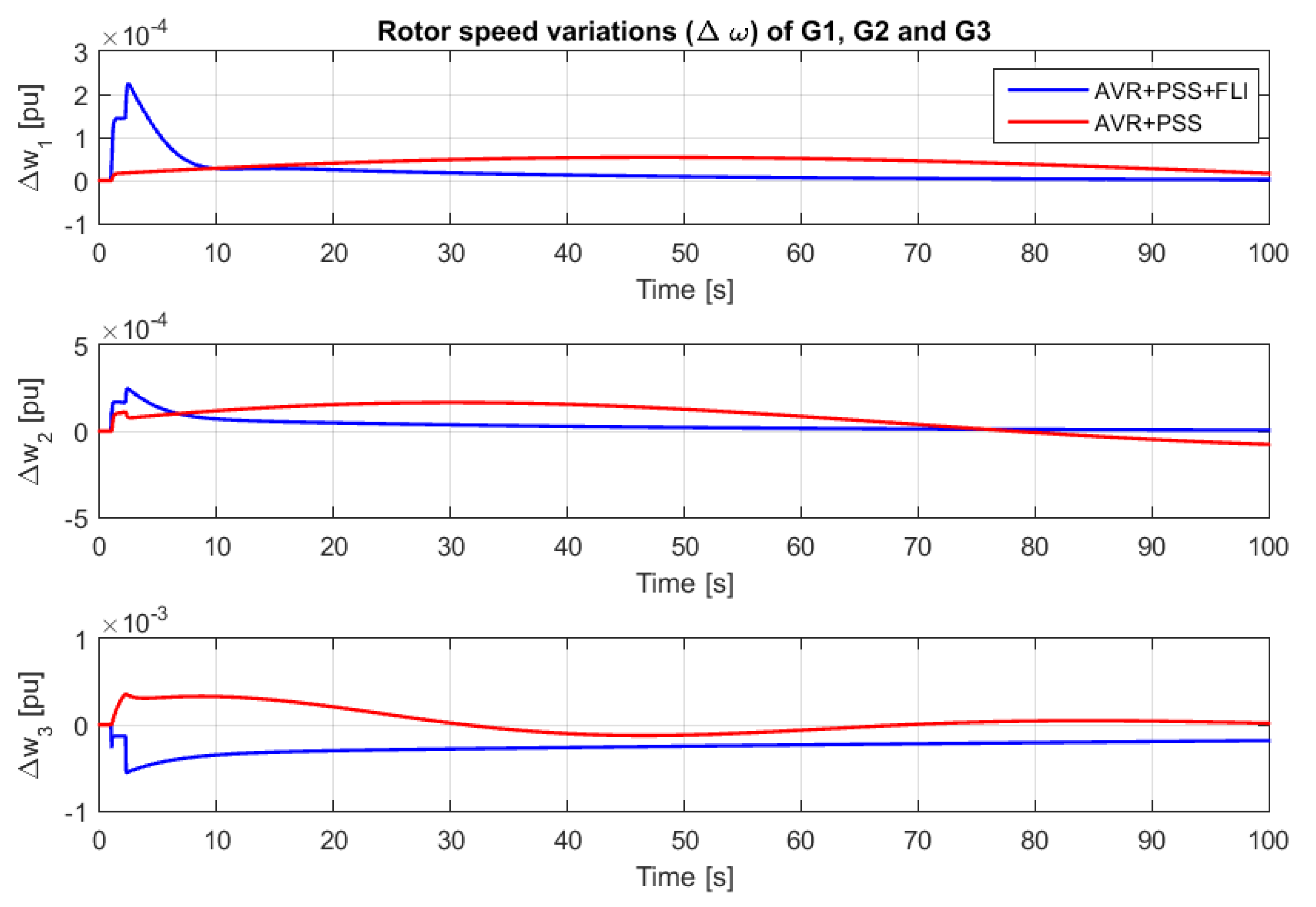
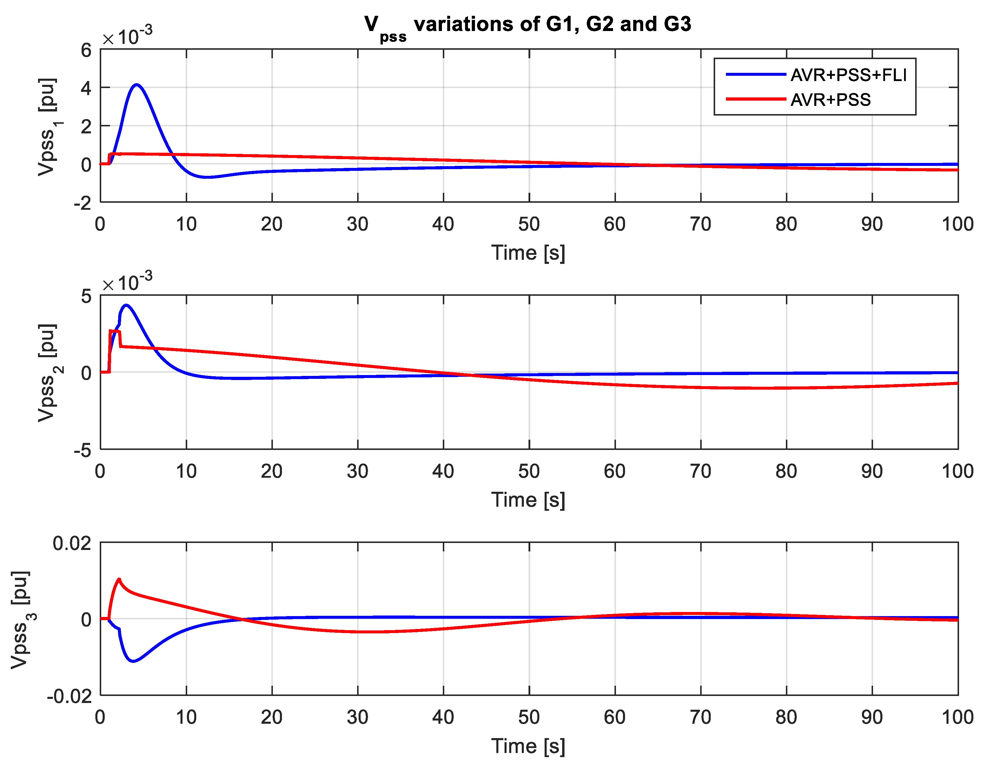
6.5. Nonlinear Time Simulations and Discussion

In order to test the applicability and robustness of the proposed UFC, a severe disturbance (described below) is applied to the system. Firstly, a high level of penetration of renewable energy occurs at t₀ = 1 s. Then, the amount of renewable energy is reduced after 20 milliseconds, i.e., at t = 1.02 s. The nonlinear simulation results obtained using the UFC together with AVR and PSS are compared with the case when only conventional AVR and PSS (AVR+PSS) are applied. Figure 8, Figure 9, Figure 10, Figure 11 and Figure 12 show the system responses corresponding to rotor angle variation, speed deviation, internal voltage deviation, field voltage and the output voltages of PSSs, respectively. From Figure 8, it is clear that the rotor angles of the machines converge much more rapidly upon the desired values when the proposed UFC is applied as opposed to conventional AVR and PSS. Moreover, it can be seen that the convergence time for the rotor angle of G3 is much greater than those of generators G1 and G2. This is due to the high inertia constant of generator G3 compared to G1 and G2, as shown in Table 2. The desired rotor angles of generators G1, G2 and G3 are 1.0251, 1.2109 and 0.13836 radians, respectively.

Figure 9 shows that the variations of angular speed with the fuzzy controller are more efficient than those with conventional regulators. In fact, it can be clearly seen that the oscillations of the fuzzy regulator are greater than those of the conventional regulator at the moment of application of the disturbances. This proves that the proposed fuzzy-based regulator responds significantly to disturbances, and is more sensitive to any fault than conventional regulators. The significant response of the proposed controller can be also observed in Figure 10, where the internal voltages underwent significant variations during the disturbances. For this reason, the field voltages of the machines contained pulses.

Figure 10 and Figure 11 also show that the proposed UFC provides good performance and achieves a rapid convergence to equilibrium in the system in comparison with the AVR and PSS regulators, despite its sensitivity to disturbances. Figure 12 shows that the output signals V_pss of the fuzzy regulator reach their steady state values faster than the signals generated by the conventional PSS regulator and with the minimum number of oscillations. Moreover, the significant reaction of the fuzzy controller during variations in operating conditions can be seen, which proves its efficiency.

Figure 13 illustrates the variations of the fuzzy control signals related to the three machines. Significant oscillations were observed when the disturbance was applied. This proves that the regulator responds effectively following a change in the system operating conditions.

Therefore, the proposed TSF modeling approach could achieve accurate representations of the studied multimachine system with a reduced number of fuzzy rules. Indeed, the nonlinear time-domain simulation proved that the proposed UFC works effectively at the moment of the application of disturbances, which is not the case for conventional stabilizers. This is due to the fact that the UFC output signal acts on all state variables, while conventional controller signals act directly on the excitation system.

7. Conclusions

Based on the fact that uncertain fuzzy models can effectively approximate systems with large numbers of nonlinearities, a new design approach for an uncertain fuzzy controller for UNS was developed in this study. In this approach, a PDC-based controller with state feedback and using Lyapunov’s direct method was implemented to stabilize the fuzzy system. Firstly, the stabilization conditions were determined without taking the system performance into account. Then, a decay rate was imposed on the decay of the Lyapunov function, which improved the dynamics of the system. Seeing that the number of fuzzy rules correlated with the number of nonlinearities, a technique for reducing the number of the latter was suggested. In this technique, all of the nonlinearities of the studied system were ranked based on their importance; then, non-significant nonlinearities were assumed to be uncertainties. This idea makes the design of fuzzy models easier and more viable. Moreover, the implementation of fuzzy controllers requires less memory and processing time. In order to test the robustness and effectiveness of the proposed controller, the UFC was applied for the stabilization of a multimachine wind farm power system. Disturbances were represented by sudden variations of wind power output. Comparisons were made between the results obtained using the UFC and those obtained with conventional PSSs and AVR regulators. The controller proposed in this study achieved an accurate representation of the system and responded effectively to changes in the system operating conditions.

It should be noted that the proposed controller could easily be applied to any other power network. In addition, the proposed modeling technique could be directly applied to multimachine systems without going through the Thevenin equivalent, which simplifies the complexity of solving such problems.

References

1. Jafari, R.; Yu, W. Fuzzy control for uncertainty nonlinear systems with dual fuzzy equations. J. Intell. Fuzzy Syst. 2015, 29, 1229–1240. [Google Scholar] [CrossRef]
2. Alshammari, B.; Salah, R.B.; Kahouli, O.; Kolsi, L. Design of fuzzy TS-PDC controller for electrical power system via rules reduction approach. Symmetry 2020, 12, 2068. [Google Scholar] [CrossRef]
3. Saadatmand, M.; Gharehpetian, G.B.; Kamwa, I.; Siano, P.; Guerrero, J.M.; Alhelou, H.H. A Survey on FOPID controllers for LFO damping in Power systems using synchronous generators, FACTS devices and inverter-based power plants. Energies 2021, 14, 5983. [Google Scholar] [CrossRef]
4. Gruenwald, B.C.; Yucelen, T.; De La Torre, G.; Jonathan, A.M. Adaptive control for uncertain dynamical systems with nonlinear reference systems. Int. J. Syst. Sci. 2020, 51, 687–703. [Google Scholar] [CrossRef]
5. Liu, Y.; Jia, T.; Niu, Y.; Zou, Y. Design of sliding mode control for a class of uncertain switched systems. Int. J. Syst. Sci. 2015, 46, 993–1002. [Google Scholar] [CrossRef]
6. Yan, T.H.; Wu, B.; He, B.; Li, W.H.; Wang, R.B. A Novel fuzzy sliding-mode control for discrete-time uncertain system. Math. Probl. Eng. 2016, 1530760, 1–9. [Google Scholar] [CrossRef]
7. Wang, R.; Li, J.; Zhang, S.; Gao, D.; Sun, H. Robust adaptive control for a class of uncertain nonlinear systems with Time-Varying Delay. Sci. World J. 2013, 2013, 963986. [Google Scholar] [CrossRef] [Green Version]
8. Pakmehr, M.; Yucelen, T. Adaptive control of uncertain systems with gain scheduled reference models and constrained control inputs. In Proceedings of the American Control Conference (ACC), Portland, OR, USA, 4–6 June 2014; IEEE: New York, NY, USA, 2014; pp. 691–696. [Google Scholar]
9. Luo, X. Design of an adaptive controller for double-fed induction wind turbine power. Energy Rep. 2021, 7, 1622–1626. [Google Scholar] [CrossRef]
10. Dong, F.; Zhao, X.; Han, J.; Chen, Y.H. Optimal fuzzy adaptive control for uncertain flexible joint manipulator based on D-operation. IET Control. Theory Appl. 2018, 12, 1286–1298. [Google Scholar] [CrossRef]
11. Zhu, Q.; Song, A.G.; Zhang, T.P.; Yang, Y.Q. Fuzzy adaptive control of delayed high order nonlinear systems. Int. J. Autom. Comput. 2012, 9, 191–199. [Google Scholar] [CrossRef]
12. Boulkroune, A.; Merazka, L.; Li, H. Fuzzy adaptive state-feedback control scheme of uncertain nonlinear multivariable Systems. IEEE Trans. Fuzzy Syst. 2019, 27, 1703–1713. [Google Scholar] [CrossRef]
13. Shen, Q.; Shi, P.; Wang, S.; Shi, Y. Fuzzy adaptive control of a class of nonlinear systems with unmodeled dynamics. Int. J. Adapt. Control Signal Process. 2019, 33, 712–730. [Google Scholar] [CrossRef]
14. Roman, R.C.; Precup, R.E.; Petriu, E.M. Hybrid data-driven fuzzy active disturbance rejection control for tower crane systems. Eur. J. Control. 2021, 58, 373–387. [Google Scholar] [CrossRef]
15. Zhu, Z.; Pan, Y.; Zhou, Q.; Lu, C. Event-triggered adaptive fuzzy control for stochastic nonlinear systems with unmeasured states and unknown backlash-like Hysteresis. IEEE Trans. Fuzzy Syst. 2021, 29, 1273–1283. [Google Scholar] [CrossRef]
16. Roy, S.; Kar, I.N. Robust time-delayed control of a class of uncertain nonlinear systems. IFAC-PapersOnLine 2016, 49, 736–741. [Google Scholar] [CrossRef]
17. Nguyen, A.T.; Laurain, T.; Palhares, R.; Lauber, J.; Sentouh, C.; Popieul, J.C. LMI-based control synthesis of constrained Takagi-Sugeno fuzzy systems subject to L2 or L∞ disturbances. Neurocomputing 2016, 207, 793–804. [Google Scholar] [CrossRef]
18. Zhang, J.; Wang, X.; Shao, X. Design and real-time implementation of Takagi–Sugeno fuzzy controller for magnetic levitation ball system. IEEE Access. 2020, 8, 38221–38228. [Google Scholar] [CrossRef]
19. Bourahala, F.; Guelton, K.; Khaber, F.; Manamanni, N. Improvements on PDC controller design for Takagi-Sugeno fuzzy systems with state time-varying delays. IFAC-PapersOnLine 2016, 49, 200–205. [Google Scholar] [CrossRef]
20. Sambariya, D.K.; Prasad, R. A Novel fuzzy rule matrix design for fuzzy logic-based power system stabilizer. Electr. Power Compon. Syst. 2017, 45, 34–48. [Google Scholar] [CrossRef]
21. Ansari, J.; Abbasi, A.R.; Heydari, M.H.; Avazzadeh, Z. Simultaneous design of fuzzy PSS and fuzzy STATCOM controllers for power system stability enhancement. Alex. Eng. J. 2022, 61, 2841–2850. [Google Scholar] [CrossRef]
22. Morère, Y. Mise en Oeuvre de lois de Commande Pour les Modèles Flous de Type Takagi-Sugeno. Ph.D. Thesis, Université de Valenciennes et du Hainaut-Cambrésis, Valenciennes, France, 2001. [Google Scholar]
23. Le Doeuff, R.; Zaïm, M.E.H. Rotating Electrical Machines; John Wiley & Sons: Hoboken, NJ, USA, 2010. [Google Scholar]
24. Lee, D.; Hu, J. Local model predictive control for T–S fuzzy systems. IEEE Trans Cybern. 2017, 47, 2556–2567. [Google Scholar] [CrossRef] [PubMed]
25. Ghadiri, H.; Khodadadi, H.; Mobayen, S.; Asad, J.H.; Rojsiraphisal, T.; Chang, A. Observer-based robust control method for switched neutral systems in the presence of interval time-varying delays. Mathematics 2021, 9, 2473. [Google Scholar] [CrossRef]
26. Guesmi, T.; Farah, A.; Abdallah, H.H.; Ouali, A. Robust design of multimachine power system stabilizers based on improved non-dominated sorting genetic algorithms. Electr Eng. 2018, 100, 1351–1363. [Google Scholar] [CrossRef]
27. Milano, F. PSAT Helps: Power System Analysis Toolbox Documentation for PSAT Version 2.0.0 _1. 2006. Available online: http://www.uclm.es/area/gsee/Web/Federico/psat.htm (accessed on 29 November 2020).
Figure 1. Thevenin equivalent circuit of a sub-system; RTh, XTh and VTh are the Thevenin equivalent circuit parameters.
Mathematics 10 01463 g001
Figure 2. Blondel diagram of a synchronous machine.
Mathematics 10 01463 g002
Figure 3. Excitation system with PSS and AVR.
Mathematics 10 01463 g003
Figure 4. Single line diagram of the WSCC system.
Mathematics 10 01463 g004
Figure 5. Flowchart of the implementation of the proposed strategy.
Mathematics 10 01463 g005
Figure 6. Block structure of the SMIB system with controllers.
Mathematics 10 01463 g006
Figure 7. Block diagram of the closed-loop system.
Mathematics 10 01463 g007
Figure 8. Rotor angle variations.
Mathematics 10 01463 g008
Figure 9. Speed deviation.
Mathematics 10 01463 g009
Figure 10. Internal voltage variations.
Mathematics 10 01463 g010
Figure 11. Field voltage variations.
Mathematics 10 01463 g011
Figure 12. Variations of PSS outputs.
Mathematics 10 01463 g012
Figure 13. Fuzzy control signal.
Mathematics 10 01463 g013