The predictive suspension algorithm is implemented on a two-axle vehicle, whose kinematics must be solved first. For simplicity, only 1/2 vehicle is modeled and symmetry action on both wheels of the same axle is assumed, so the problem becomes bi-dimensional. The vehicle will travel through a deterministic topography. Hence, the vertical position of any wheel can be established from the horizontal position by the function that relates both variables.
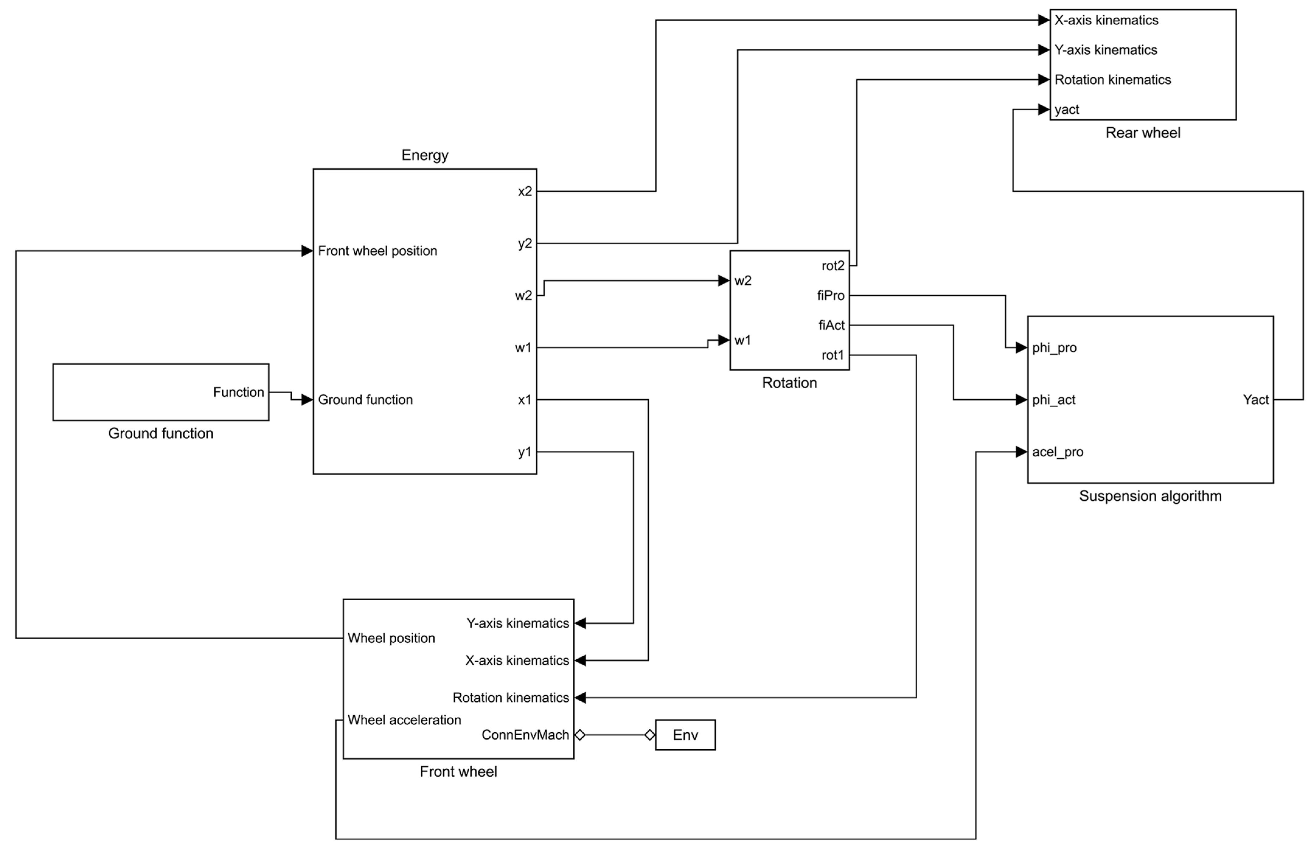
The vehicle model also assumes that the mechanical energy remains constant, only wheels have mass and pure rolling (no sliding) is considered as it is a condition for the good performance of the suspension algorithm. This model and the algorithm were implemented in Simulink.
2.1. Vehicle Model
The mechanical energy of the vehicle is given by Equation (1)
where
E is the mechanical energy,
m1 and
m2 are the masses of both wheels,
I1 and
I2 are the inertias of both wheels,
v1 and
v2 are the linear velocities of the wheels,
ω1 and
ω2 are the angular speeds of the wheels,
y1 and
y2 are the vertical positions of the wheels and
g is the gravity.
By assuming pure rolling motion and the wheels as solid disks, Equation (1) can be simplified; therefore, the initial energy of the system is obtained from Equation (2), where the subscript 0 means “initial conditions”.
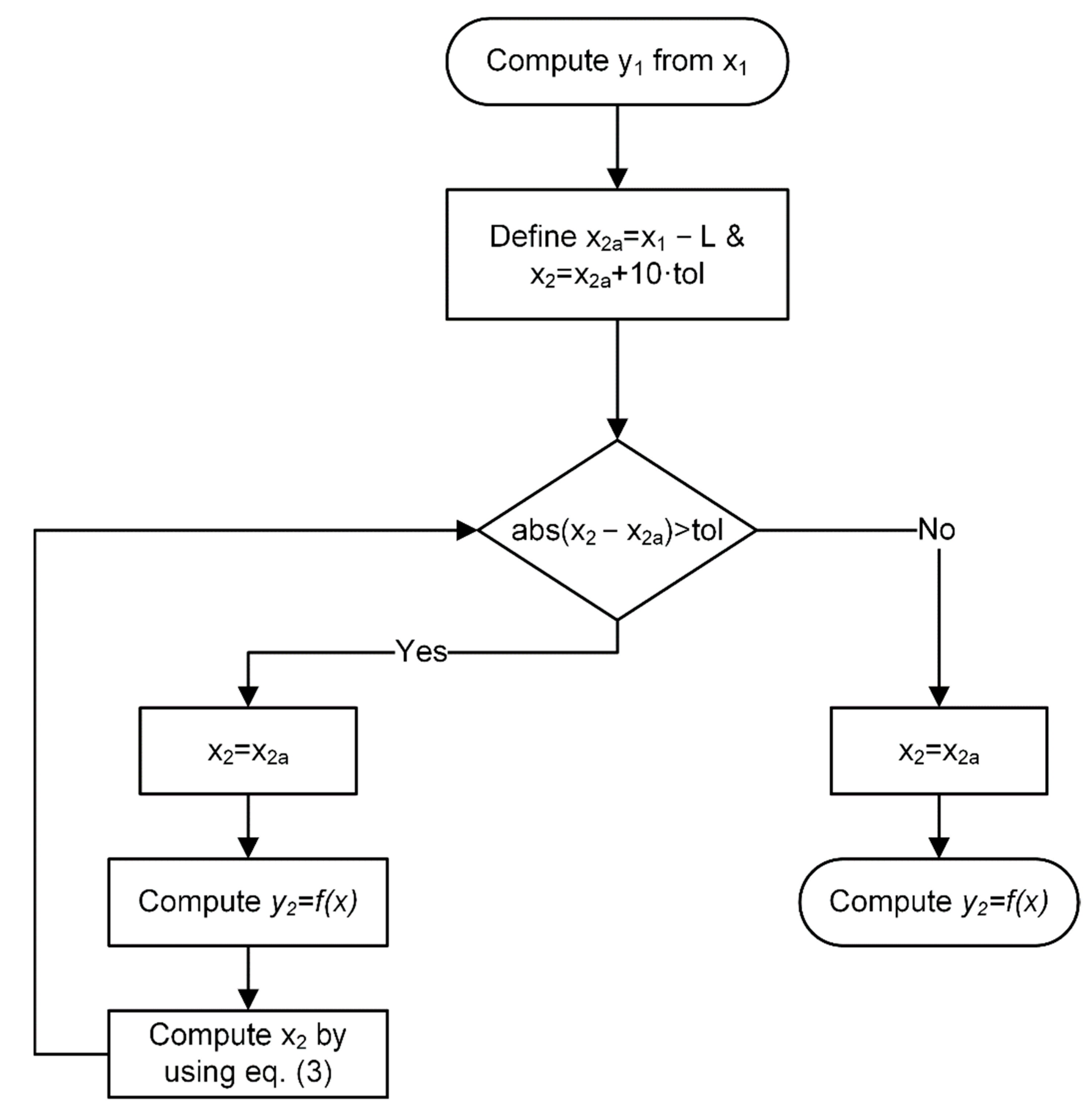
The distance between the front and rear wheels (that is, the wheelbase)
L is known and can be described mathematically as a circumference centered on the front wheel and radius
L. The position of the rear wheel is obtained by computing the intersection of this circumference with the trajectory described by the ground function
y = f(x). Hence, the solution of the equation system given by Equation (3) yields the position of the rear wheel.
This system of equations is solved by iteration, as the ground function can be any type of function, even not analytical. The flowchart describing the iteration process is shown in
Figure 1.
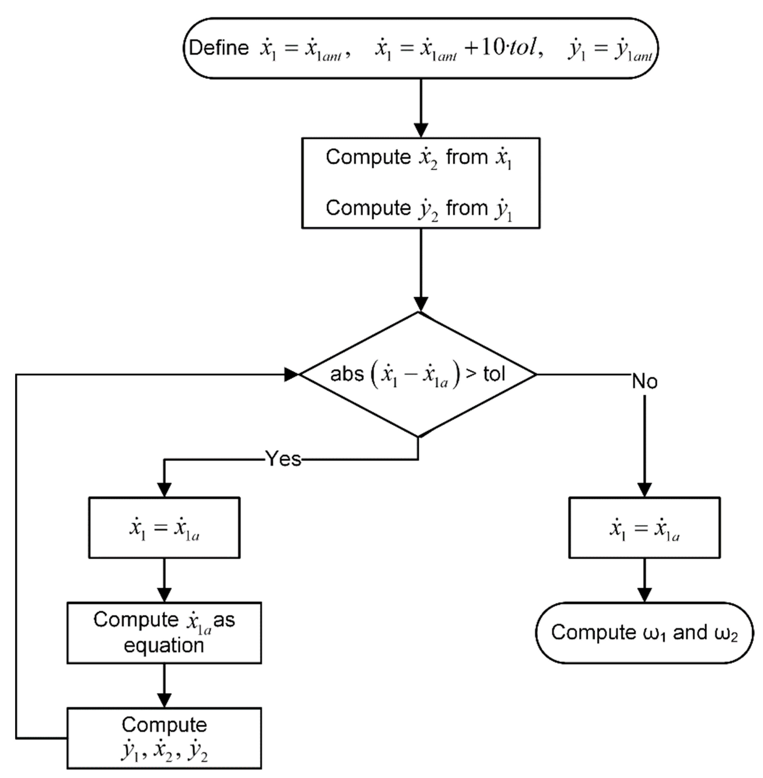
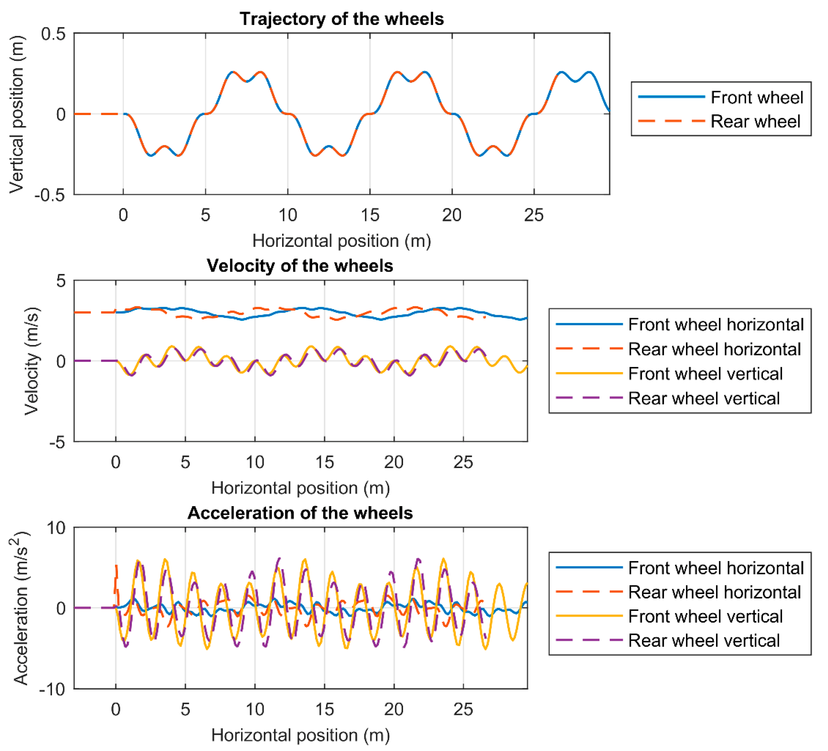
The velocity of both wheels is computed from the conservation of energy, the time derivative of the constraint equation and the ground function, obtaining the equation system built up by Equations (4)–(6).
In order to solve this system more efficiently, polar coordinates are used. This implies defining the pitch angle
θ as Equation (7).
Therefore, the constraint Equation (3) is rewritten as Equation (8).
The combination of the conservation of energy with the time derivatives of the ground function and the constraint equation in polar coordinates yields Equations (9)–(12), which allows computing all the components of the speed of both wheels.
As previously, this system of equations is solved by iteration following the flowchart in
Figure 2.
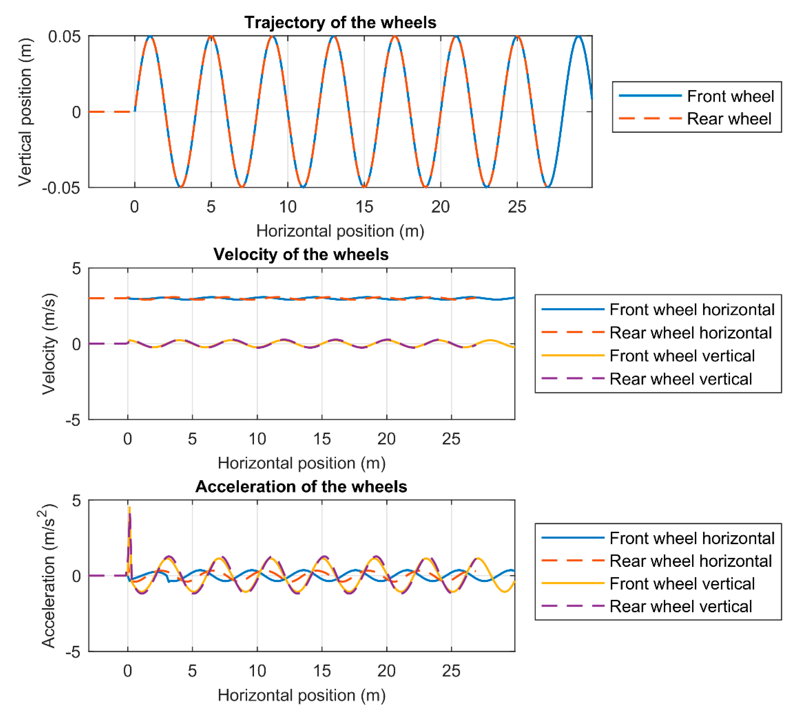
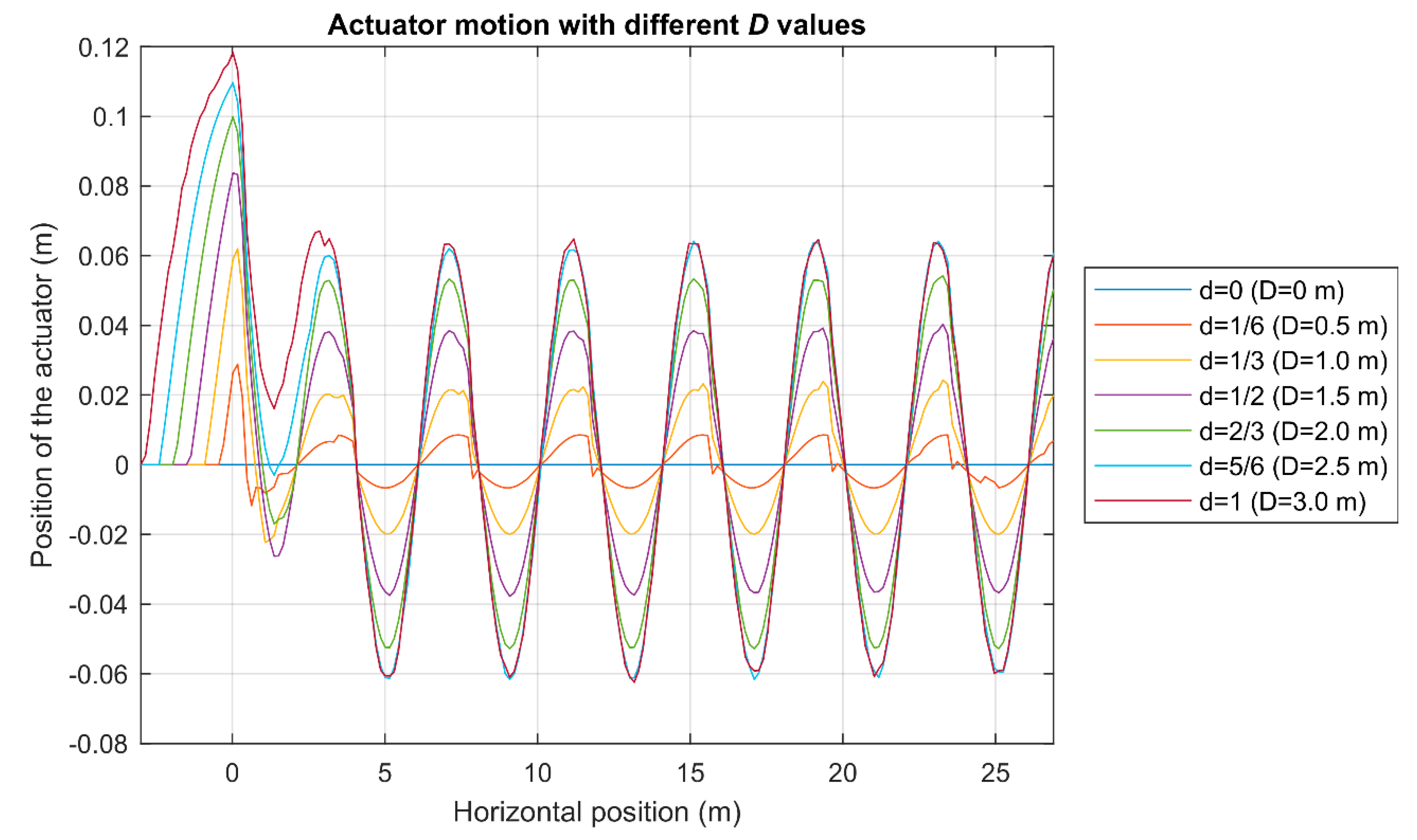
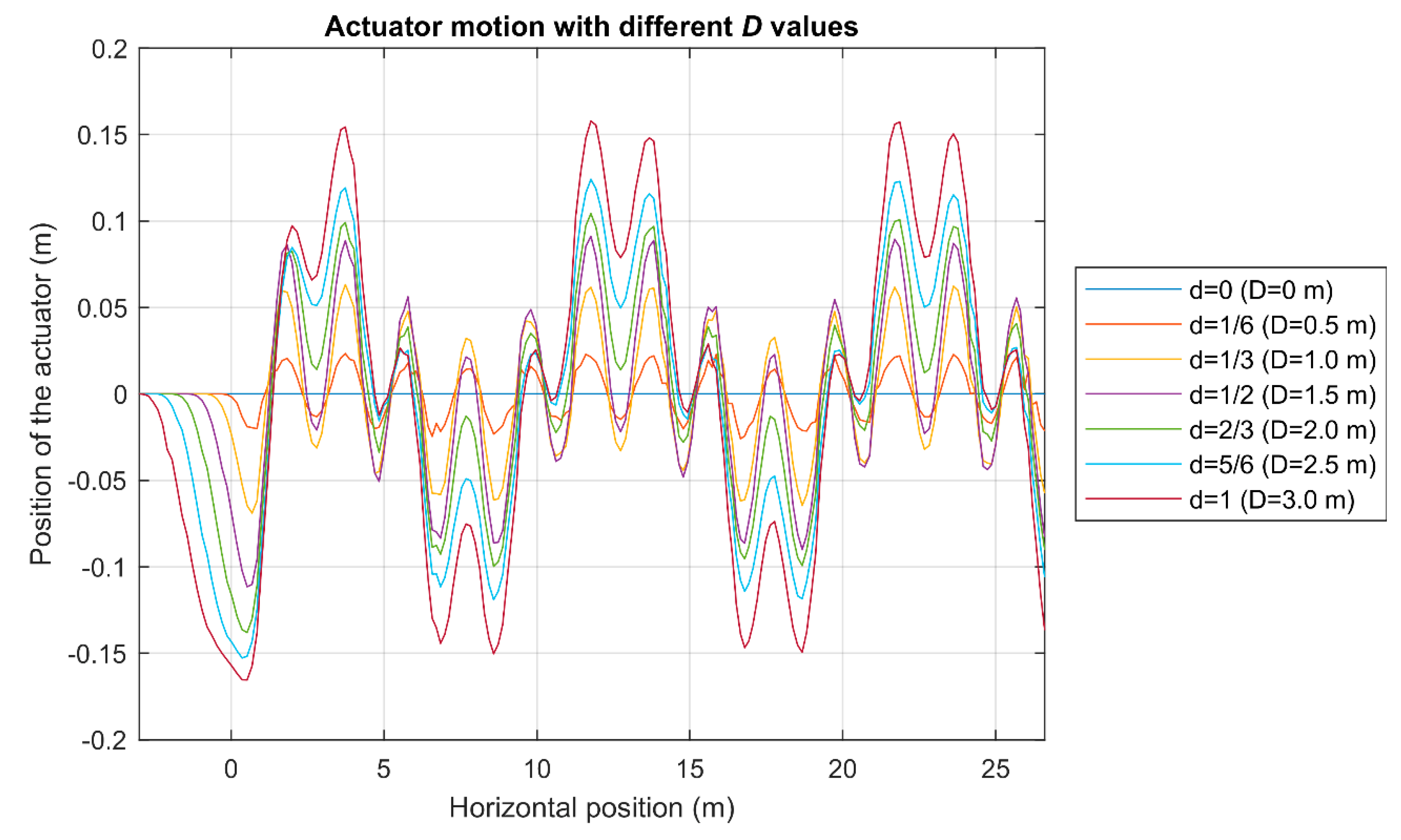
Two different ground topographies and several values of the parameter
D were proposed for testing the algorithm. The first topography (profile 1) simulates a wiggly surface and is defined by Equation (13)—where A
1 is the amplitude of the wave and λ
1 is the wavelength, both in meters.
The second profile is a combination of two sinusoidal irregularities according to Equation (14):
A1 and
A2 are the amplitudes of both sines,
λ1 and
λ2 are the wavelengths,
A0 is the reference height and
a is a parameter to guarantee continuity in the first derivative; therefore,
A0 and
a are such that:
The model parameters and initial conditions used in the simulations of both topography profiles are summarized in
Table 1. The input values of both topography profiles are depicted in
Table 2, as well as the computed values of variables
A0 and
a.
2.2. Suspension Algorithm
The suspension algorithm is applied to the 1/2 vehicle model described in the previous subsection. The frontwheel acts as a probe wheel, whereas the rear wheel is the actuated wheel. The probe wheel is instrumented with a vertical accelerometer and both wheels should be equipped with an accurate system for measuring their angular positions.
In
Figure 3, two kinds of terrain defects (peak and corrugated) are sketched, as well as the trajectories described by the wheel centers and the trajectory that the sprung mass should follow (a straight line).
Let Δ
t be the sampling time interval of the accelerometer and
the vertical acceleration registered at time
t = nΔ
t. Assuming a constant vertical jerk along the interval [
(n-1)Δ
t,
nΔ
t] yields Equation (17).
Then the expressions for the vertical velocity and position of the wheel center are, respectively:
Although the corresponding velocity and position errors grow with time, nΔt, and time squared, (nΔt)2, respectively, (easy to show); this is not too much of a problem since the algorithm does not include the absolute height, but its variation over a certain distance, “D”. In other words, the database of values obtained in Equations (18) and (19), will be dynamically refreshed, so that n, and therefore the temporal interval nΔt, does not increase indefinitely.
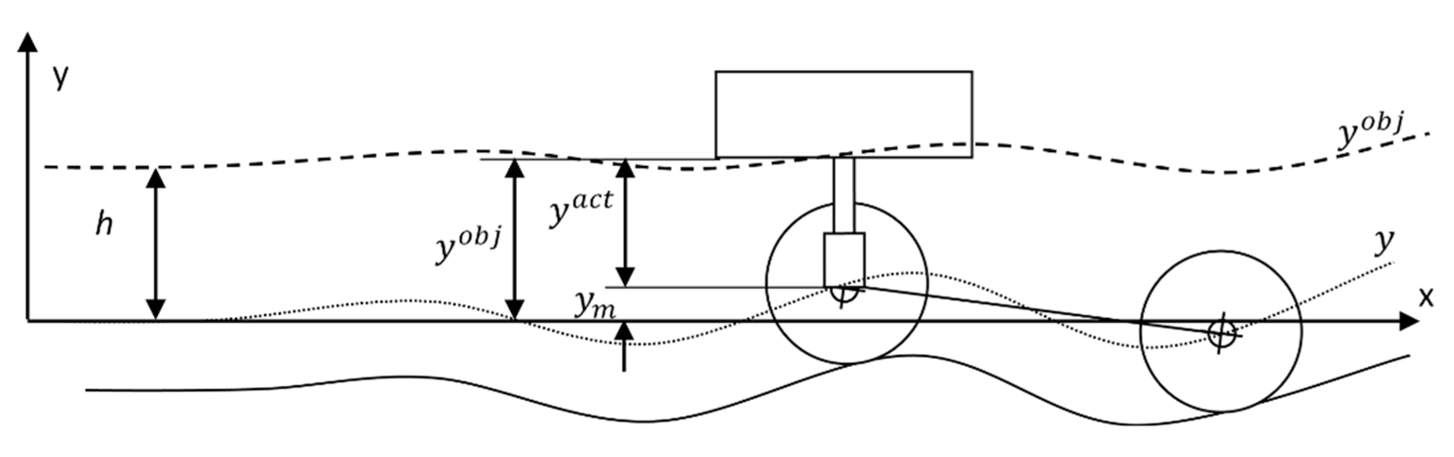
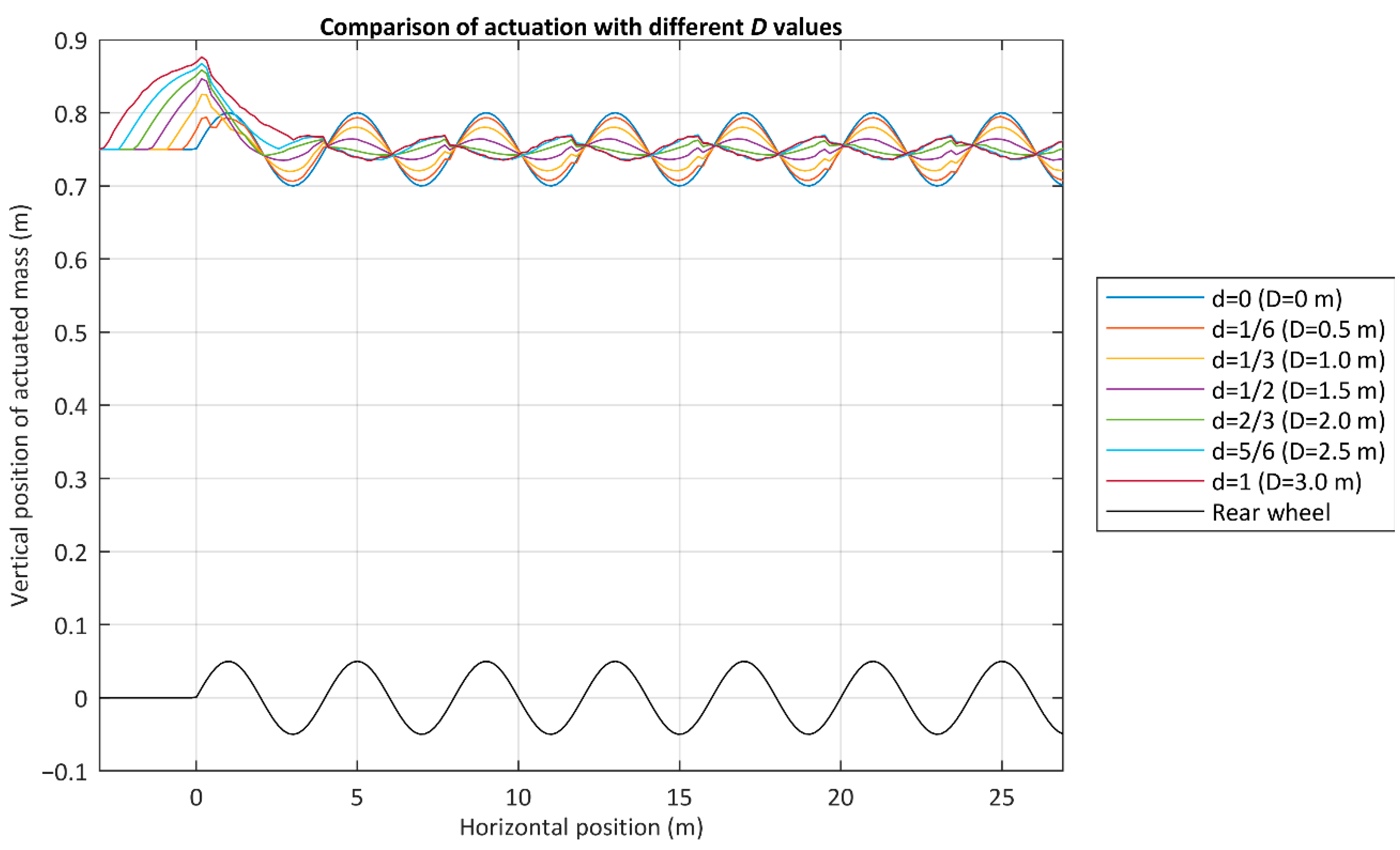
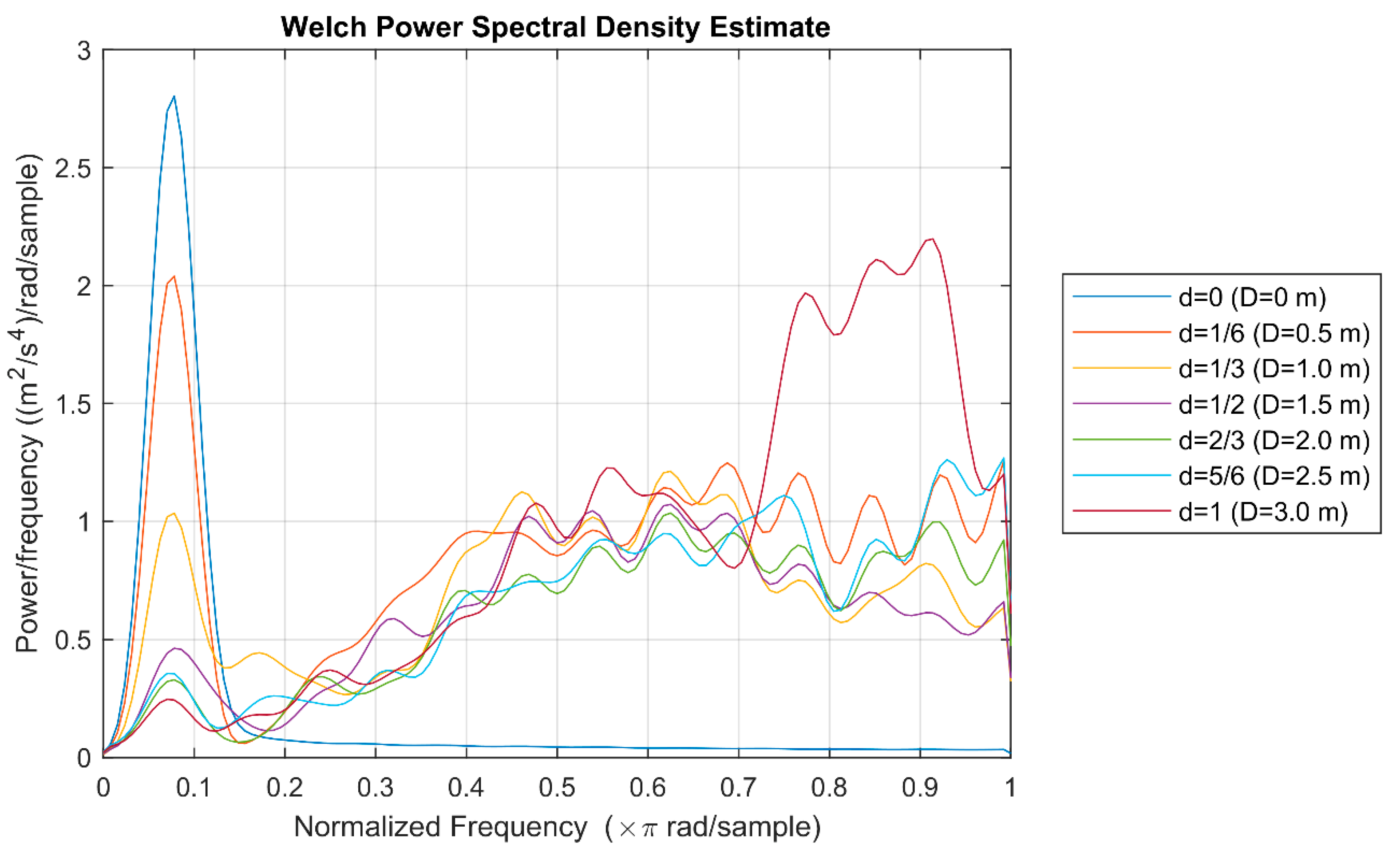
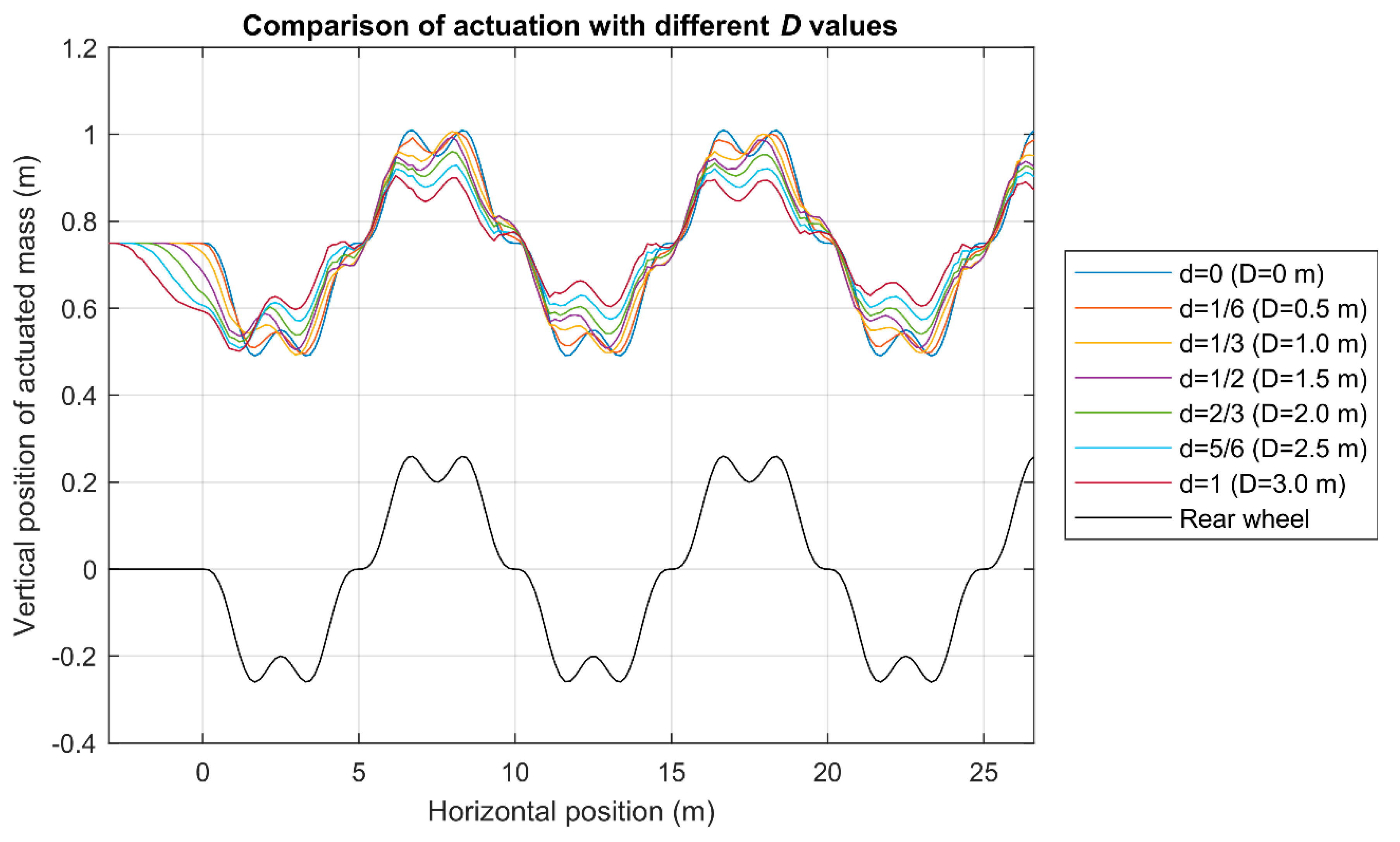
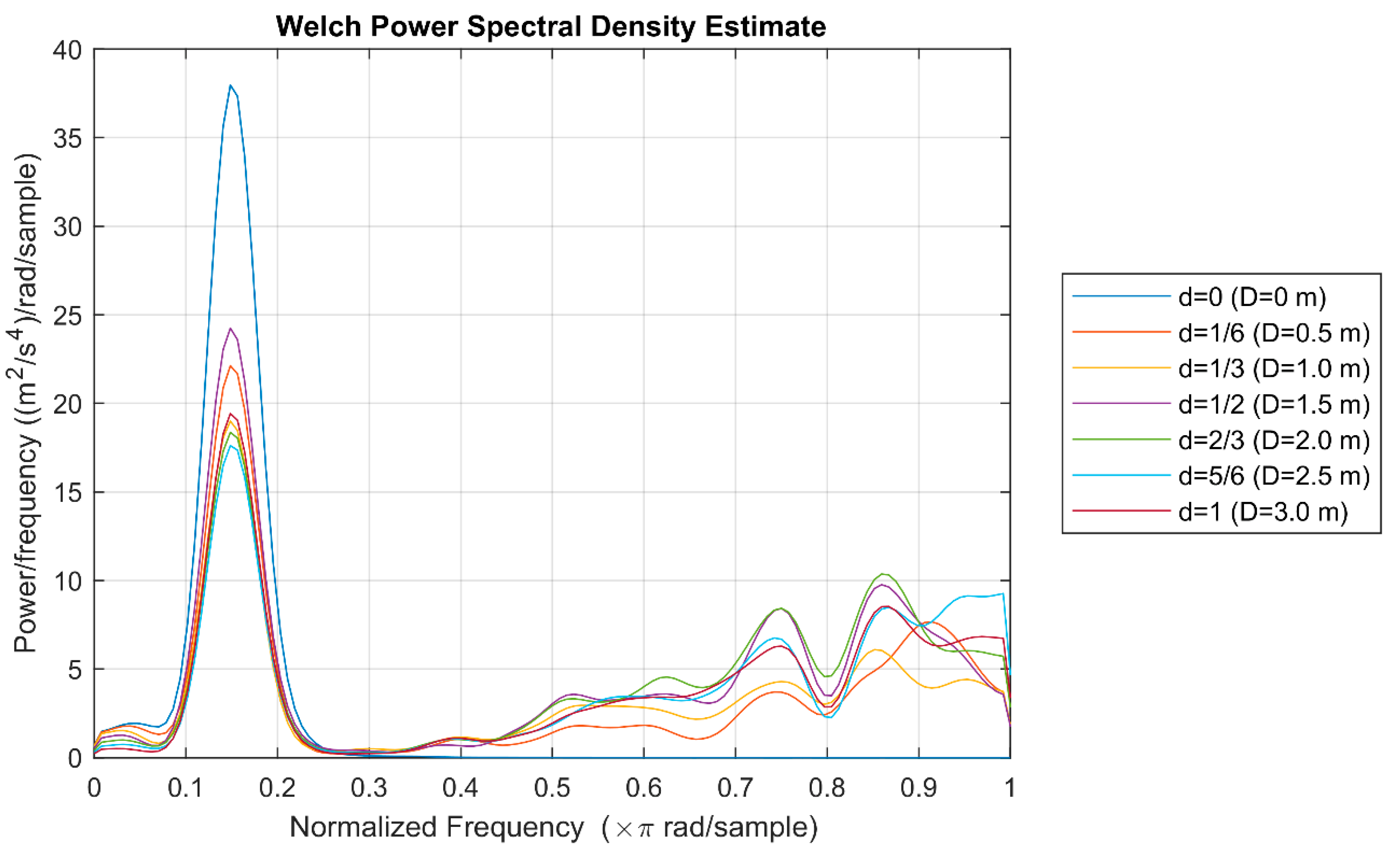
The vertical actuator (between the actuated or rear wheel and the sprung mass) has to maintain the latter at the objective height. In this approach, the objective height is the result of the moving average of the calculated height over the rolling distance 2D. Actually, the larger this distance, the softer the objective function, but also the bigger error is accumulated in calculating the height from the accelerometer reading. Thus, parameter “D” should be adjusted according to the kind of roughness the topography has (with the sole requirement not to exceed the distance between wheels).
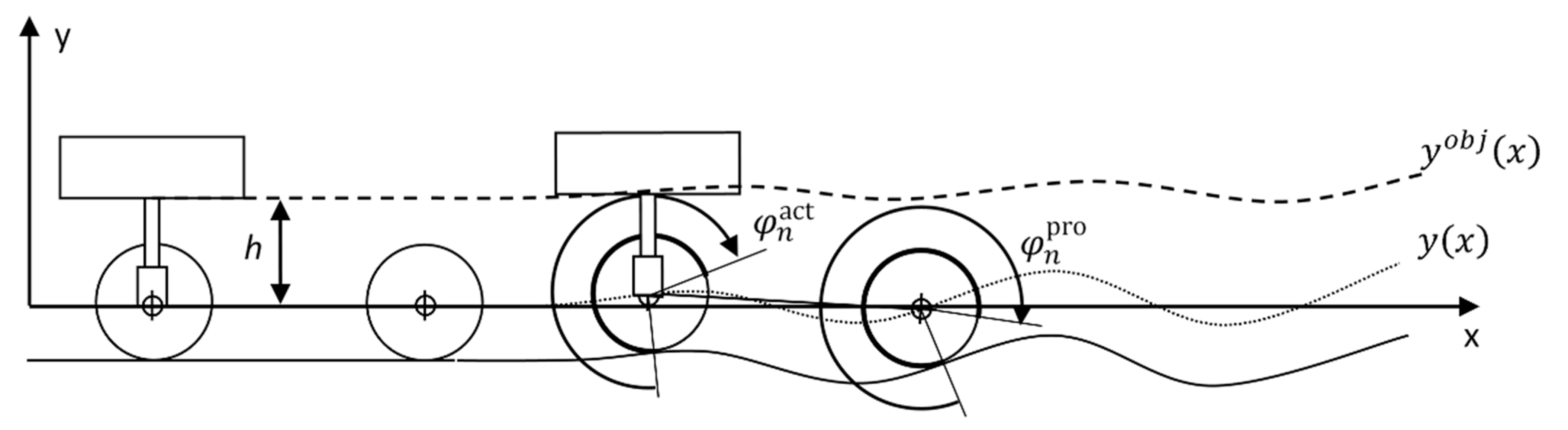
For the proposed algorithm, it is important to know exactly the position of both wheels (which are supposed to roll without slipping) on the ground. This is achieved by recording the corresponding angles,
(angle turned by the probe wheel, and actuated wheel, respectively), having set both to zero at the initial position (
n = 0). The model is sketched in
Figure 4 at the initial position and at the time
t = nΔ
t. The actual trajectories followed by the center of the wheels and the trajectory the end of the actuator should follow are also represented.
At time
t =
nΔ
t, the vertical acceleration of the probe wheel,
, and the angles turned by the wheels, are measured. Then, the velocity,
, and vertical position,
, are calculated by using Equations (18) and (19), respectively. All these values are recorded in a database in the way indicated in
Table 3.
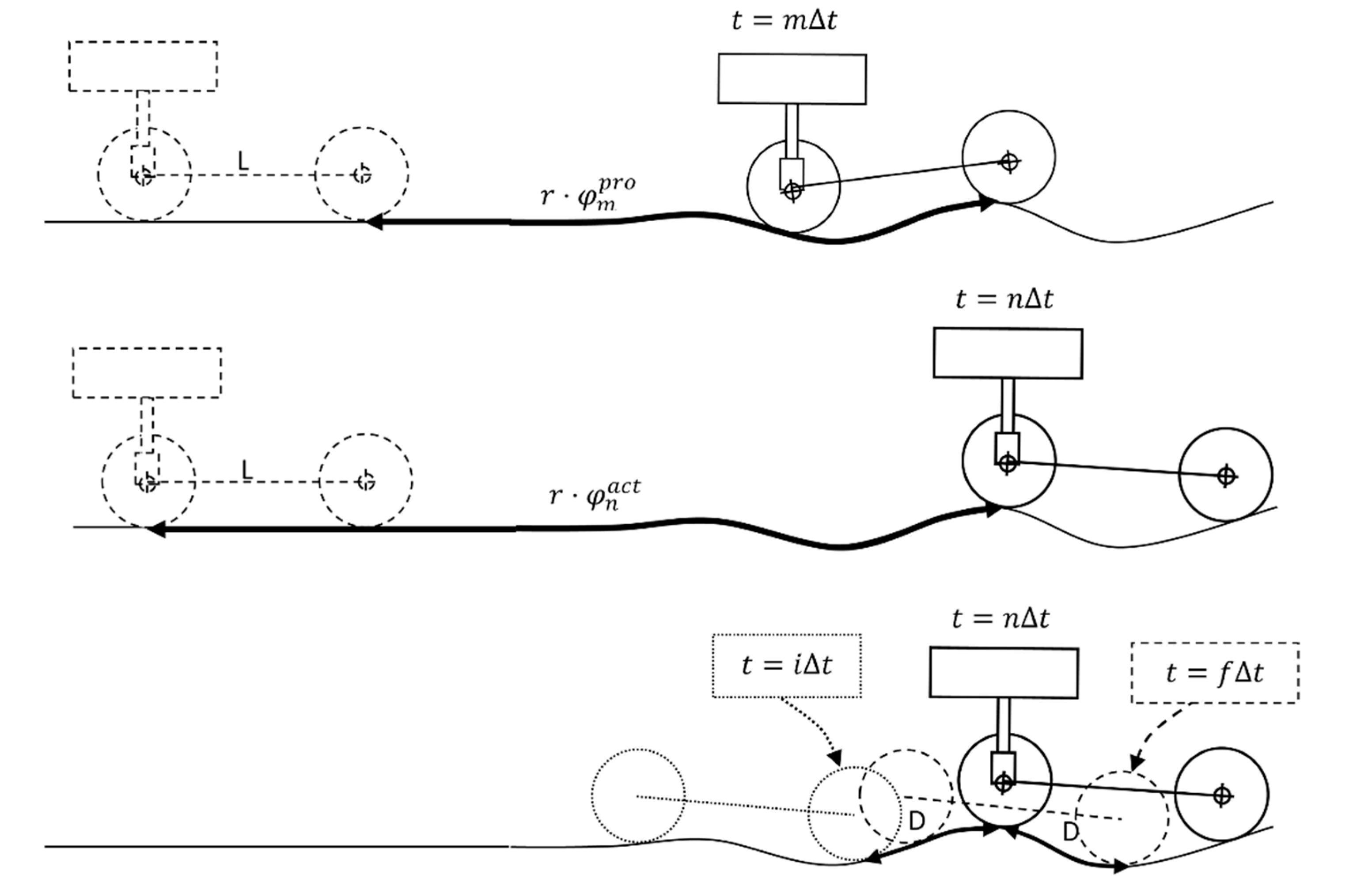
Once enough records have been acquired, the algorithm is ready to provide the current length to be taken by the actuator. The objective height is calculated as the moving average centered on the record corresponding to the actuated wheel and over a sufficient number of records; speaking in terms of rolling distances, the moving average is calculated over a rolling distance of 2
D. This is achieved by identifying the records
m,
i and
f that, respectively, define the current position for the actuated wheel and the first and last of the records to average over. In other words, at
t =
mΔ
t the probe wheel was just on the same point of the trajectory that the actuated wheel is at
t =
nΔ
t (i.e., at present). In
Figure 5, the model at moments corresponding to records
m, n, i and
f is sketched.
On seeing
Figure 5, if we consider both wheels have the same radius,
r, the following rules for identifying the numbers
m, i and
f are deduced:
With “≈” we mean “is the nearest value to” (note that is a discrete set of values, so in general, none of the last equalities could be exactly satisfied). We have also considered that the first section of the trajectory is flat and horizontal, with a minimum distance that is equal to the wheelbase, L.
Once the records
i, m and
f have been identified, the algorithm calculates the objective height (see
Figure 6) as:
and the actuated distance results:
where
h is the initial objective height (i.e., the actuator initial length, see
Figure 4 and
Figure 6).
Finally, the database is refreshed by deleting the records with subscripts less than
i, and decreasing the remainder subscripts in
i units:
In this way, the database does not grow indefinitely, and only the records to be used by the algorithm at the current time of calculation remain.
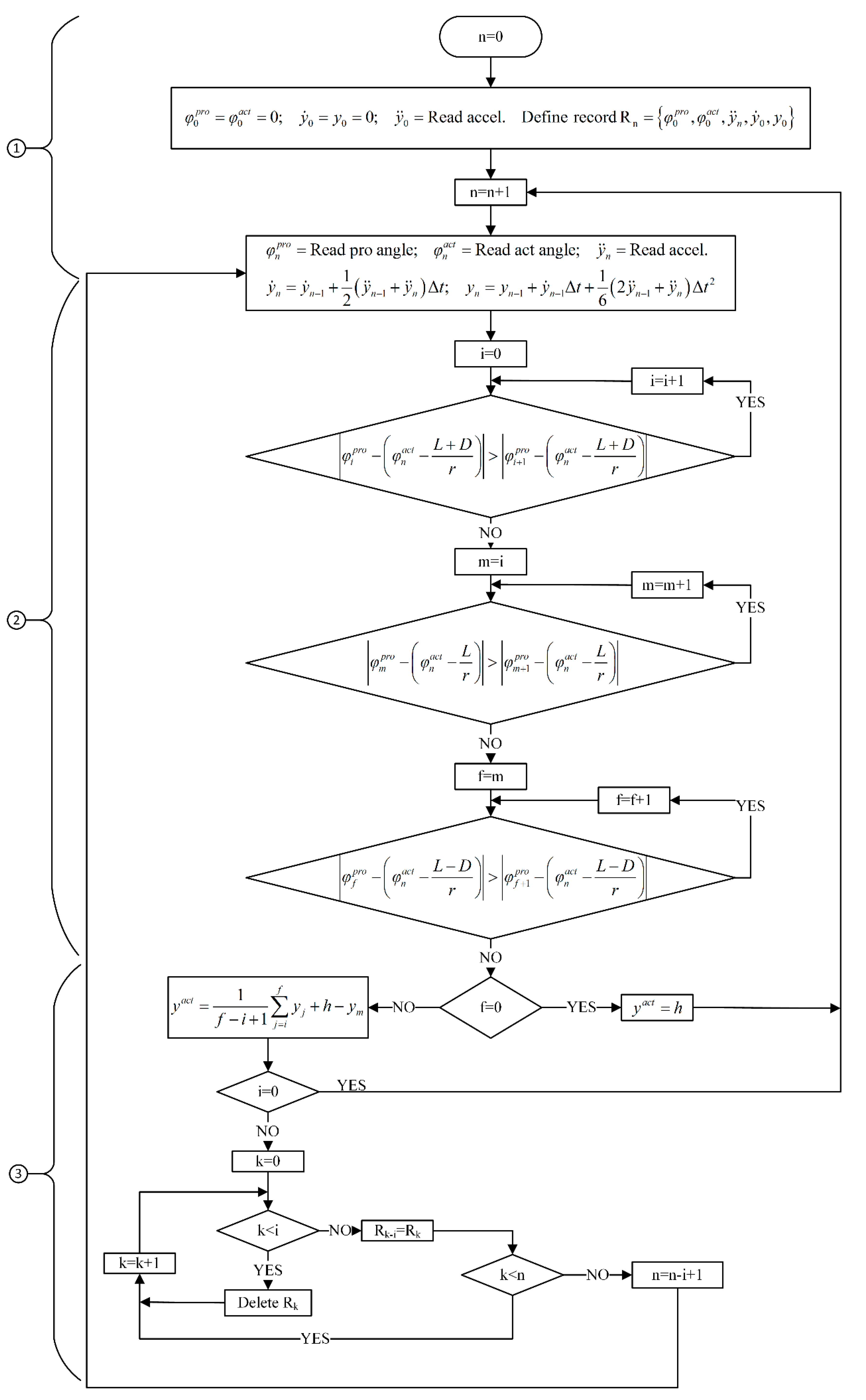
In summary, the algorithm can be considered as consisting of three tasks:
Reading (angles and vertical acceleration) and computing vertical velocity and position.
Identifying the indexes i, m and f.
Obtaining the actuated distance and refreshing the database.
To understand how the algorithm performs the second task, suppose the database at time
nΔ
t is as shown in
Table 4. For a given angle turned by the actuated wheel
, the algorithm computes the theoretical angle turned by the probe wheel at the three key moments
iΔ
t,
mΔ
t and
fΔ
t (,
and
, respectively), using Equations (20)–(22).Then, it searches the closest actual angles recorded in the database to those computed and determines the indexes
i,
m and
f. As the probe wheel angle turned does not decrease with
n (hence
i ≤ m ≤ f), the search can be performed sequentially.
The whole algorithm flowchart is represented in
Figure 7.


