Abstract
In this paper, a cubic Hermite spline interpolating scheme reproducing both linear polynomials and hyperbolic functions is considered. The interpolating scheme is mainly defined by means of integral values over the subintervals of a partition of the function to be approximated, rather than the function and its first derivative values. The scheme provided is everywhere and yields optimal order. We provide some numerical tests to illustrate the good performance of the novel approximation scheme.
MSC:
65D07
1. Introduction
Nowadays, numerical methods are a common tool, just a click away from the user. Interpolation is a particular and very important numerical method, which is widely used to address the solution of theoretical problems and show their full potential to numerically solve problems that occur in many different branches of science, engineering and economics.
The interpolation approximants should be easily evaluated, differentiated and integrated. Spline functions, i.e., smooth piecewise polynomial functions, fulfil all these requirements.
Since the introduction of the systematic study of spline functions by I. J. Schoenberg in the 1940s [1], they have become an indispensable tool in approximation theory and numerical computation, including computer-aided geometric design (CAGD) [2,3], the numerical solution of PDEs, numerical quadratures, interpolation and quasi-interpolation, regularization, least squares, isogeometric analysis and image processing.
Spline functions have been the subject of many research results that have been presented in well-known books [4,5]. Furthermore, thousands of papers related to spline functions and their applications have been published in the last five years, in fields ranging from computer science, engineering, physics and astronomy to entertainment and conceptual design assistance.
Polynomial spline functions are the most commonly used class, especially due to the fact that they admit normalized bases on any bounded interval (Bernstein bases and B-spline bases); for more details, see [5,6,7,8]. Indeed, Bernstein bases and B-splines possess several interesting properties, such as non-negativity, local support, partition of unity and totally positive bases [9]. Bernstein basis functions of degree n are the best among all bases of the polynomial space of degree less than or equal to n. This means that it is the basis relative to which the control polygon of any curve yields the best information on the curve itself. The non-polynomial B-splines have also been studied in the literature. For instance, the trigonometric B-splines were presented in [10,11]. The authors in [12] have established a recurrence relation for the trigonometric B-splines of arbitrary order. A complete construction of exponential tension B-splines of arbitrary order was given in [13]. A more recent study on this kind of spline was given in [14,15]. The splines associated with the exponential B-spline space are often referred to as hyperbolic splines [16].
Unfortunately, neither Bernstein bases nor B-splines are suitable to perfectly describe conic sections, which are shapes of major interest in certain engineering applications. This resulted in the introduction of NURBS [17], which can be seen as a generalization of B-splines, inheriting from them important properties and with the additional benefit of making possible the exact representation of conic sections. On the other hand, the NURBS representation suffers from some drawbacks that are considered critical in CAD. In fact, the necessity of weights does not have an evident geometric meaning and their selection is often unclear. Furthermore, it behaves awkwardly with respect to differentiation and integration, which are indispensable operators in analysis. On this concern, it is sufficient to think about the complex structure of the derivative of a NURBS curve of a given order.
An alternative is to use the so-called generalized B-splines; see [18,19] and references therein. The generalized B-splines belong to the extended space spanned by , where and are smooth functions. The two functions and can be selected to achieve the exact representation of salient profiles of interest and/or to obtain particular features. The most popular choices of these functions are: and , which yield algebraic trigonometric and algebraic exponential splines, respectively. The algebraic exponential splines are often referred as algebraic hyperbolic splines. Algebraic trigonometric and hyperbolic splines allow an exact representation of conic sections, as well as of some transcendental curves, such as helix and cycloid curves. In fact, they are in a position to provide parametrizations of conic sections that are significantly more related to the arc length than NURBS.
These classes of splines are also known as cycloidal spaces, and they have become the subjects of a considerable amount of research [2,20,21,22,23,24,25,26]. The algebraic hyperbolic spaces spanned by the functions 1, x, …, , , , for , have been widely considered in the literature; see [21] and references quoted. They yield the tension splines, which are extremely useful for avoiding undesirable oscillations in the interpolation curves [27].
In this paper, we consider the algebraic hyperbolic (AH) cubic spline space, spanned by , and let be a uniform partition of a bounded interval , with . Given values , , , there exists a unique cubic AH Hermite interpolant such that , , . The spline s defined from the local interpolants is a continuous AH spline that interpolates the data .
In this work, we suppose that the data , , , are not given, and we assume that the integral values over subintervals , are given. Then, our purpose is the construction of the Hermite interpolant s using only this information. This kind of approximation arises in various fields, such as mechanics, mathematical statistics, electricity, environmental science, climatology, oceanography and so on (for more details, see References [28,29] and references therein). More precisely, the values will be computed by means of smoothness conditions at the knots and the integral values over subintervals . This is done by solving a three-diagonal linear system. Some final conditions are required. In particular, we assume that the three values , and or are given. In general, these three values are not always available. We suggest a modified scheme that does not involve any final conditions to avoid this limitation.
Integro spline approximation was treated in various works in the literature. The author in [30,31] developed two types of integro spline approximants, cubic and quintic cases, respectively. The two schemes introduced in [30,31] require various end conditions and the solution of a three-diagonal system of linear equations. Solving a linear system of equations sometimes is very expensive, so the authors in [32] developed cubic integro splines quasi-interpolant without solving any system of equations. An integro quartic spline scheme has been constructed in [33]. The authors in [21,34] provided some integro spline schemes for the case of non-polynomial splines. More recent work on the integro spline approximation is given in [35,36]
In this work, a new class of integro spline approximant is introduced. The proposed operator is smooth everywhere and exactly reproduces both linear polynomials and hyperbolic functions, which is useful to avoid undesirable oscillations in curves’ interpolation. Some end conditions are needed, and to avoid this inconvenience, we have proposed a modified scheme that does not require additional end conditions.
This paper is organized as follows: in Section 2, we first present the cubic AH interpolating scheme, which is defined by means of the value and the derivative value at each knot of the partition. We also study the error bound of the presented scheme. Then, the conditions for achieving the smoothness are described. Thus, an approach to define the integro spline scheme by means of integral values is proposed. In Section 3, we provide some numerical tests. Finally, we present some conclusions.
2. Algebraic Hyperbolic Spline Interpolation
Let be a uniform partition of a bounded interval , with .
2.1. Cubic Algebraic Hyperbolic (AH) Splines of Class
The construction of a cubic AH spline interpolant on the partition should be locally expressed in each sub-interval in terms of the function and the first derivative values of the approximated function at knots and .
The space of cubic AH splines on with global continuity is denoted as
where stands for the linear space of cubic AH splines. Its dimension equals . The following Hermite interpolation problem can then be considered: there exists a unique spline such that
for any given set of -values. Therefore, each spline restricted to the sub-interval can be represented as follows:
in which , , are classical Hermite basis functions of restricted to the sub-interval . The basis functions , , are the unique solution of the interpolation problem given by (1) in , where , , and , respectively. More precisely,
They can be expressed as follows:
where .
Figure 1 shows the typical plots of the basis functions , , , on the sub-interval .
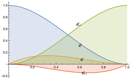
Figure 1.
Plots of the basis functions on .
Consider that the values of are related to an explicit function f, i.e., , . Then, it holds that
In order to prove this statement, consider an arbitrary but fixed value different from and , and define
in which the constant is chosen such that , that is,
The function R has at least three roots in , which are , and .
According to Rolle’s theorem, has at least two roots in that are different from , , and also , which means that has at least four roots in . Analogously and progressively, it is shown that has three roots in the interval , has two and has only one root, say . It then states
It holds that
This proves Equation (3).
The proposed interpolant s is defined from the values and first derivative values at the break points. Unfortunately, this dataset is not always at hand. This paper deals with the case where neither the values nor the derivative values are known. Instead, we assume that the integral values over the sub-intervals are available.
The strategy pursued in this work is the following: we first highlight the relationship between function and first derivative values by imposing the smoothness at the set of break points. Next, we express the derivative values in the mean integral values provided.
The smoothness of at , yields the following consistency relations:
where and .
The error related to the approximation scheme (4) can be derived from the following result.
Lemma 1.
Let ; then, the local truncation errors , , associated with the scheme (4) are given by the expressions
Proof.
The function f is supposed to be of class , that is,
Using Equation (4), it results that
By replacing , and by their Taylor expansions, the intended result can be achieved, which completes the proof. □
The next result can be easily deduced from the previous lemma.
Theorem 2.
Let , then
At this point, we have simply provided a scheme that approximates the derivative values from the function values by imposing smoothness at the break points. In what follows, we will deal with the case where the function values themselves are not available, whereas the integrals over the sub-intervals are known.
2.2. Cubic Algebraic Hyperbolic Spline Interpolant Based on Mean Integral Value
In traditional spline interpolation problems, it is assumed that the function values at the knots are given. In this subsection, the function values are supposed to be unknowns and we assume that the integrals over the sub-intervals , are provided and are equal to
In the sequel, we will provide a scheme that approximates derivative values from the integrals , .
By integrating s over and , one can obtain
respectively.
Subtracting (6) from (7) as a first step, and then applying (4) as a second step, allows us to eliminate the unknowns , as well as to achieve new relations that link only the unknowns with the provided data . It results that
with
This yields a system of linear equations, while there are unknowns . Then, two additional end conditions are required to determine the unknowns. The end conditions are the first derivative values at the end points a and b. Assume that and are provided. Then, a linear tridiagonal system results.
with .
The following result shows that the linear system (9) has a unique solution.
Theorem 3.
For , the matrix system in (9) is a strictly diagonally dominant matrix.
Proof.
Let . It is easy to show that . Indeed, a simple calculation gives us the following equality:
Since , then , which completes the proof. □
The LU factorization is adequate for solving (9) because the index on the diagonally dominant property of the matrix A is equal to for small enough . In fact, let be the matrix coefficient of system (9). The index on the diagonally dominant property of matrix A is given by
Its limit when h is close to zero is equal to .
Once the values of , are determined, we can then compute , by means of (6). However, we still need another end condition. Suppose that one of the values and is provided; then, we can start from it and use (6) to obtain the remaining unknowns in an iterative way.
To analyze the interpolation error, we need the following lemma to establish an error bound for our operator.
Lemma 4.
Let ; then, the local truncation errors , , associated with the scheme (9), are given by the expressions
Theorem 5.
Proof.
Consider the sub-interval . Let p be the spline in , which satisfies , . Then, it results that
This due to the fact that , which concludes the proof. □
In the general context, the end conditions may not be provided. Thus, to avoid this limitation, we will provide explicit expressions for the end conditions , and by means of integral values.
Lemma 6.
For a given function ,
Proof.
The Taylor expansion of f around a is as follows:
Therefore, the following system is obtained:
Through a straightforward computation, we can obtain the expressions of and .
By the same approach, we can obtain the expression of , which concludes the proof. □
3. Numerical Results
This section provides some numerical results to illustrate the performance of the above Hermite interpolation operator. To this end, we will use the test functions
whose plots appear in Figure 2. The two first functions are the 1D versions of the Franke [37] and Nielson [38] functions.
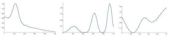
Figure 2.
Plots of test functions: (left), (center) and (right).
Let us consider the interval . The tests are carried out for a sequence of uniform mesh associated with the break points , n, where .
The interpolation error is estimated as
where , 200, are equally spaced points in I. The estimated numerical convergence order (NCO) is given by the rate
In Table 1, the estimated quasi-interpolation errors and NCOs for functions , and are shown.

Table 1.
Estimated errors for functions , and , and NCOs with different values of n.
Now, we will compare the numerical method proposed here with the results obtained with different methods in other papers in the literature, although the test functions in these papers are extremely simple, namely
In Table 2 and Table 3, we list the resulting errors for the approximation of the functions and , respectively, by using the cubic spline operator provided here and those in References [34,39,40]. Table 2 and Table 3 show that the novel numerical scheme improves the results in References [34,39,40].
Table 2.
Estimated errors for function , and NCOs with different values of n.
Table 3.
Estimated errors for function , and NCOs with different values of n.
Next, we deal with the following four test functions also defined on :
Their typical plots are shown in Figure 3.
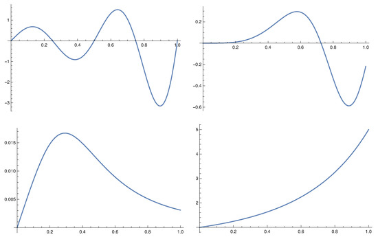
Figure 3.
Plots of test functions: , , and (from (left) to (right) and from (top) to (bottom)).
Our goal now is to compare the method introduced herein with the methods that use only algebraic splines, as well as those that combine the features of algebraic and hyperbolic functions. To this end, we consider the approaches presented by A. Boujraf et al. in [29], D. Barrera et al. in [21], J. Wu and X. Zhang in [40] and S. Eddargani et al. in [34], so we implement the approaches described in [29,34,40] to be able to execute any test function, because those involved in the cited references are simple examples and one of them (exponential function) is reproduced by our approach.
In Table 4 and Table 5, we list the resulting errors for the approximation of the functions and , respectively, using our approach and the one provided in [29]. Table 6 shows the resulting errors for the approximation of the function , using the approach described here and those in References [21,34,40]. In Table 7, we list the resulting errors for the approximation of the function by using the approach provided here and those in References [34,40].
Table 4.
Estimated errors for function , and NCOs with different values of n.
Table 5.
Estimated errors for function , and NCOs with different values of n.
Table 6.
Estimated errors for function , and NCOs with different values of n.
Table 7.
Estimated errors for function , and NCOs with different values of n.
It is clear that the proposed scheme improves the results in the previous papers by at least two orders of magnitude. Consequently, in certain contexts, it is highly recommended to use splines that benefit from the features of both algebraic and hyperbolic functions instead of using only the features of algebraic ones.
4. Conclusions
Approximation from integral values represents a critical topic because of its extensive application in many different areas. This paper considers a cubic Hermite spline interpolant that reproduces linear polynomials and hyperbolic functions. The proposed interpolant is everywhere and is defined from the value and the first derivative value at each knot of the partition. The function and derivative values are assumed to be unknowns, and then they are determined using the smoothness conditions and the mean integral values. The numerical results illustrate the good performance of the novel approximation scheme. The construction used herein requires the resolution of a system of linear equations, which can be computationally expensive, especially when dealing with a large number of data. Future work will address the issue of avoiding this limitation.
Author Contributions
Supervision, A.L. and M.L.; Writing—original draft, M.O.; Writing—review & editing, S.E. All authors have read and agreed to the published version of the manuscript.
Funding
The first author acknowledges partial financial support by the Department of Applied Mathematics of the University of Granada.
Institutional Review Board Statement
Not applicable.
Informed Consent Statement
Not applicable.
Data Availability Statement
Not applicable.
Acknowledgments
The authors wish to thank the anonymous referees for their very pertinent and useful comments, which helped them to improve the original manuscript. The first author would like to thank the Department of Applied Mathematics of the University of Granada for the financial support for the research stay during which this work was carried out. The authors wish to thank the Hassan First University of Settat for the financial aid offered for the final cost of the APC.
Conflicts of Interest
The authors declare no conflict of interest.
References
- Schoenberg, I.J. Contributions to the problem of approximation of equidistant data by analytic functions. Part A. on the problem of smoothing or graduation. A first class of analytic approximation formulae. Q. Appl. Math. 1946, 4, 45–99. [Google Scholar] [CrossRef]
- Zheng, J.Y.; Hu, G.; Ji, X.M.; Qin, X.Q. Quintic generalized Hermite interpolation curves: Construction and shape optimization using an improved GWO algorithm. Comput. Appl. Math. 2022, 41, 1–29. [Google Scholar] [CrossRef]
- Ammad, M.; Misro, M.Y.; Abbas, M.; Majeed, A. Generalized Developable Cubic Trigonometric Bézier Surfaces. Mathematics 2021, 9, 283. [Google Scholar] [CrossRef]
- Schumaker, L.L. Spline Functions: Basic Theory; Cambridge Mathematical Library; Cambridge University Press: Cambridge, UK, 2007; pp. I–Vi. [Google Scholar]
- De Boor, C. A Practical Guide to Splines. In Applied Mathematical Sciences; Springer: Berlin/Heidelberg, Germany, 1978; Volume 27. [Google Scholar]
- Barrera, D.; Eddargani, S.; Lamnii, A. A novel construction of B-spline-like bases for a family of many knot spline spaces and their application to quasi-interpolation. J. Comput. Appl. Math. 2022, 404, 113761. [Google Scholar] [CrossRef]
- Barrera, D.; Eddargani, S.; Ibáñez, M.J.; Lamnii, A. A new approach to deal with C2 cubic splines and its application to super-convergent quasi-interpolation. Math. Comput. Simul. 2022, 194, 401–415. [Google Scholar] [CrossRef]
- Ershov, S.N. B-Splines and Bernstein Basis Polynomials. Phys. Part. Nuclei Lett. 2019, 16, 593–601. [Google Scholar] [CrossRef]
- Yu, Y.Y.; Ma, H.; Zhu, C.G. Total positivity of a kind of generalized toric-Bernstein basis. Linear Algebra Appl. 2019, 579, 449–462. [Google Scholar] [CrossRef]
- Koch, P.; Lyche, T.; Neamtu, M.; Schumaker, L. Control curves and knot insertion for trigonometric splines. Adv. Comput. Math. 1995, 3, 405–424. [Google Scholar] [CrossRef]
- Walz, G. Identities for trigonometric B-splines with an application to curve design. BIT 1997, 37, 189–201. [Google Scholar] [CrossRef]
- Lyche, T.; Winther, R. A stable recurrence relation for trigonometric B-splines. J. Approx. Theory 1979, 25, 266–279. [Google Scholar] [CrossRef]
- Koch, P.E.; Lyche, T. Construction of exponential tension B-splines of arbitrary order. In Curves and Surfaces; Laurent, P.J., Le Méhauté, A., Schumaker, L.L., Eds.; Academic Press: New York, NY, USA, 1991; pp. 255–258. [Google Scholar]
- Conti, C.; Gemignani, L.; Romani, L. Exponential Pseudo-Splines: Looking beyond Exponential B-splines. J. Math. Anal. Appl. 2016, 439, 32–56. [Google Scholar] [CrossRef]
- Campagna, R.; Conti, C.; Cuomo, S. Smoothing exponential-polynomial splines for multi-exponential decay data. Dolomites Res. Notes Approx. 2019, 12, 86–100. [Google Scholar]
- Campagna, R.; Conti, C. Penalized hyperbolic-polynomial splines. Appl. Math. Lett. 2021, 118, 107159. [Google Scholar] [CrossRef]
- Yang, X. Fitting and fairing Hermite-type data by matrix weighted NURBS curves. Comput.-Aided Des. 2018, 102, 22–32. [Google Scholar] [CrossRef]
- Speleers, H. Algorithm 1020: Computation of Multi-Degree Tchebycheffian B-Splines. ACM Trans. Math. Softw. 2022, 48, 1–31. [Google Scholar] [CrossRef]
- Liu, X.; Divani, A.A.; Petersen, A. Truncated estimation in functional generalized linear regression models. Comput. Stat. Data Anal. 2022, 169, 107421. [Google Scholar] [CrossRef]
- Eddargani, S.; Lamnii, A.; Lamnii, M.; Sbibih, D.; Zidna, A. Algebraic hyperbolic spline quasi-interpolants and applications. J. Comput. Appl. Math. 2019, 347, 196–209. [Google Scholar] [CrossRef]
- Barrera, D.; Eddargani, S.; Lamnii, A. Uniform algebraic hyperbolic spline quasi-interpolant based on mean integral values. Comp. Math. Methods 2021, 3, e1123. [Google Scholar] [CrossRef]
- Carnicer, J.M.; Mainar, E.; Peña, M. Interpolation on cycloidal spaces. J. Approx. Theory 2014, 187, 18–29. [Google Scholar] [CrossRef]
- Mazure, L. From Taylor interpolation to Hermite interpolation via duality. Jaen J. Approx. 2012, 4, 15–45. [Google Scholar]
- Ait-Haddou, R.; Mazure, M.L.; Ruhland, H. A remarkable Wronskian with application to critical lengths of cycloidal spaces. Calcolo 2019, 56, 45–56. [Google Scholar] [CrossRef]
- Barrera, D.; Eddargani, D.; Lamnii, A.; Oraiche, M. On non polynomial monotonicity-preserving C1 spline interpolation. Comp. Math. Methods 2021, 3, e1160. [Google Scholar] [CrossRef]
- Ajeddar, M.; Lamnii, A. Smooth reverse subdivision of uniform algebraic hyperbolic B-splines and wavelets. Int. J. Wavelet Multiresolut. Inf. Process. 2021, 19, 2150018. [Google Scholar] [CrossRef]
- Marusic, M.; Rogina, M. Sharp error-bounds for interpolating splines in tension. J. Comput. Appl. Math. 1995, 61, 205–223. [Google Scholar] [CrossRef][Green Version]
- Delhez, E. A spline interpolation technique that preserve mass budget. Appl. Math. Lett. 2003, 16, 17–26. [Google Scholar] [CrossRef]
- Boujraf, A.; Sbibih, D.; Tahrichi, M.; Tijini, A. A simple method for constructing integro spline quasi-interpolants. Math. Comput. Simul. 2015, 15, 36–47. [Google Scholar] [CrossRef]
- Behforooz, H. Approximation by integro cubic splines. Appl. Math. Comput. 2006, 175, 8–15. [Google Scholar] [CrossRef]
- Behforooz, H. Interpolation by integro quintic splines. Appl. Math. Comput. 2010, 216, 364–367. [Google Scholar] [CrossRef]
- Zhanlav, T.; Mijiddorj, R. Integro cubic splines and their approximation properties. Appl. Math. Ser. Tver State Univ. Russia 2008, 26, 65. [Google Scholar] [CrossRef]
- Lang, F.G.; Xu, X.P. On integro quartic spline interpolation. J. Comput. Appl. Math. 2012, 236, 4214. [Google Scholar] [CrossRef]
- Eddargani, S.; Lamnii, A.; Lamnii, M. On algebraic trigonometric integro splines. Z. Angew. Math. Mech. 2020, 100, e201900262. [Google Scholar] [CrossRef]
- Mijiddorj, R.; Zhanlav, T. Algorithm to construct integro splines. ANZIAM J. 2021, 63, 359–375. [Google Scholar]
- Zhanlav, T.; Mijiddorj, R. Integro cubic splines on non-uniform grids and their properties. East Asian J. Appl. Math. 2021, 11, 406–420. [Google Scholar]
- Franke, R. Scattered data interpolation: Tests of some methods. Math. Comp. 1982, 38, 181–200. [Google Scholar]
- Nielson, G.M. A first order blending method for triangles based upon cubic interpolation. Int. J. Numer. Meth. Eng. 1978, 15, 308–318. [Google Scholar] [CrossRef]
- Zhanlav, T.; Mijiddorj, R. The local integro cubic splines and their approximation properties. Appl. Math. Comput. 2010, 216, 2215–2219. [Google Scholar] [CrossRef]
- Wu, J.; Zhang, X. Integro quadratic spline interpolation. Appl. Math. Model. 2015, 39, 2973–2980. [Google Scholar] [CrossRef]


Publisher’s Note: MDPI stays neutral with regard to jurisdictional claims in published maps and institutional affiliations. |
© 2022 by the authors. Licensee MDPI, Basel, Switzerland. This article is an open access article distributed under the terms and conditions of the Creative Commons Attribution (CC BY) license (https://creativecommons.org/licenses/by/4.0/).