Abstract
In this paper, we introduce a new line search technique, then employ it to construct a novel accelerated forward–backward algorithm for solving convex minimization problems of the form of the summation of two convex functions in which one of these functions is smooth in a real Hilbert space. We establish a weak convergence to a solution of the proposed algorithm without the Lipschitz assumption on the gradient of the objective function. Furthermore, we analyze its performance by applying the proposed algorithm to solving classification problems on various data sets and compare with other line search algorithms. Based on the experiments, the proposed algorithm performs better than other line search algorithms.
Keywords:
forward–backward algorithm; line search; accelerated algorithm; convex minimization problems; data classification; machine learning MSC:
65K05; 90C25; 90C30
1. Introduction
The convex minimization problem in the form of the sum of two convex functions plays a very important role in machine learning. This problem has been analyzed and studied by many authors because of its applications in various fields such as data science, computer science, statistics, engineering, physics, and medical science. Some examples of these applications are signal processing, compressed sensing, medical image reconstruction, digital image processing, and data prediction and classification; see [1,2,3,4,5,6,7,8].
As we know in machine learning, especially in data prediction and classification problems, the main objective is to minimize loss functions. Many loss functions can be viewed as convex functions; thus by employing convex minimization, one could find the minimum of such functions, which in turn solve data prediction and classification problems. Many works have implemented this strategy; see [9,10,11] and the references therein for more information. In this work, we apply extreme learning machine together with the least absolute shrinkage and selection operator to solve classification problems; more detail will be discussed in a later section. First, we introduce a convex minimization problem, which can be formulated as the following form:
where is proper, convex differentiable on an open set containing and is a proper, lower semicontinuous convex function defined on a real Hilbert space H.
A solution of (1) is in fact a fixed point of the operator , i.e.,
where and which is known as the forward–backward operator. In order to solve (1), the forward–backward algorithm [12] was introduced as follows:
where is a positive number. If is L-Lipschitz continuous and , then a sequence generated by (3) converges weakly to a solution of (1). There are several techniques that can improve the performance of (3). For instance, we could utilize an inertial step, which was first introduced by Polyak [13], to solve smooth convex minimization problems. Since then, there have been several works that included an inertial step in their algorithms to accelerate the convergence behavior; see [14,15,16,17,18,19] for examples.
One of the most famous forward–backward-type algorithms that implements an inertial step is the fast iterative shrinkage–thresholding algorithm (FISTA) [20]. It is defined as the following Algorithm 1.
| Algorithm 1. FISTA. |
|
The term is known as an inertial term with an inertial parameter . It has been shown that FISTA performs better than (3). Later, other forward–backward-type algorithms have been introduced and studied by many authors; see for instance [2,8,18,21,22]. However, most of these works assume the Lipschitz assumption on , which is difficult for computation in general. Therefore, in this paper, we focus on another approach where is not necessarily Lipschitz continuous.
In 2016, Cruz and Nghia [23] introduced a line search technique as the following Algorithm 2.
| Algorithm 2. Line search 1. |
|
They asserted that Line Search 1 stops after finitely many steps and proposed the following Algorithm 3.
| Algorithm 3. Algorithm with Line Search 1. |
|
They also showed that the sequence defined by Algorithm 3 converges weakly to a solution of (1) under Assumptions A1 and A2 where:
- A1.
- are proper lower semicontinuous convex functions with
- A2.
- f is differentiable on an open set containing and is uniformly continuous on any bounded subset of and maps any bounded subset of to a bounded set in
It is noted that the L-Lipschitz continuity of is not necessarily assumed. Moreover, if is L-Lipschitz continuous, then A2 is satisfied.
In 2019, Kankam et al. [3] proposed the new line search as the following Algorithm 4.
| Algorithm 4. Line search 2. |
|
They also asserted that Line Search 2 stops at finitely many steps and proposed the following Algorithm 5.
| Algorithm 5. Algorithm with Line Search 2. |
|
A weak convergence result of this algorithm was obtained under Assumptions A1 and A2. Although Algorithms 3 and 5 obtained weak convergence results without the Lipschitz assumption on , the two algorithms did not utilize an inertial step yet. Therefore, some improvements of their convergence behavior using this technique are interesting to investigate.
Motivated by the works mentioned earlier, we aim to introduce a new line search technique and prove that it is well-defined. Then, we employ it to construct a novel forward–backward algorithm that utilizes an inertial step to improve its performance to be better than the other line search algorithms. We prove a weak convergence theorem of the proposed algorithm without the Lipschitz assumption on and apply it to solve classification problems on various data sets. We also compare its performance with Algorithms 3 and 5 to show that the proposed algorithm performs better.
This work is organized as follows: In Section 2, we recall some important definitions and lemmas used in later sections. In Section 3, we introduce a new line search technique and algorithm for solving (1). Then, we analyze the convergence and complexity of the proposed algorithm under Assumptions A1 and A2. In Section 4, we apply the proposed algorithm to solve data classification problems and compare its performance with other algorithms. Finally, the conclusion of this work is presented in Section 5.
2. Preliminaries
In this section, some important definitions and lemmas, which will be used in later sections, are presented.
Let be a sequence in H and . We denote and as a strong and weak convergence of to x, respectively. Let be a proper lower semicontinuous and convex function. We denote .
A subdifferential of f at x is defined by
A proximal operator is defined as follows:
where I is an identity mapping and is a positive number. It is well known that this operator is single-valued, nonexpansive, and
see [23] for more details. Next, we present some important lemmas for this work.
Lemma 1
([24]). Let be a subdifferential of f. Then, the following hold:
- (i)
- is maximal monotone;
- (ii)
- is demiclosed, i.e., for any sequence such that and then .
Lemma 2
([25]). Let be proper lower semicontinuous convex functions with and Then, for any and we have
Lemma 3
([26]). Let H be a real Hilbert space. Then, for all and the following hold:
- (i)
- (ii)
- (iii)
- (iv)
Lemma 4
([8]). Let and be sequences of non-negative real numbers such that
Then, the following holds:
Moreover, if then is bounded.
Lemma 5
([26]). Let and be sequences of non-negative real numbers such that
If and then exists.
Lemma 6
([27], Opial). Let be a sequence in a Hilbert space H. If there exists a nonempty subset Ω of H such that the following hold:
- (i)
- For any exists;
- (ii)
- Every weak-cluster point of belongs to
Then, converges weakly to an element in Ω.
3. Main Results
In this section, we define a new line search technique and a new accelerated algorithm with the new line search for solving (1). We denote the set of all solutions of (1) and suppose that are two convex functions that satisfy Assumptions A1 and A2, and is closed. Furthermore, we also suppose that .
We first introduce a new line search technique as the following Algorithm 6.
| Algorithm 6. Line Search 3 . |
|
We first show that Line Search 3 terminates at finitely many steps.
Lemma 7.
Line Search 3 stops at finitely many steps.
Proof.
If , then , so Line Search 3 stops with zero steps. If , suppose by contradiction that, for all the following hold:
or
Then, from these assumptions, we can find a subsequence of such that (5) or (6) holds. First, we show that
are bounded. It follows from Lemma 2 that
for all In combination with A2, we conclude that is bounded. Next, we prove that is bounded. Since is nonexpansive, for any , then
for all ; hence, is bounded. Again, it follows from A2 that is bounded. To complete the proof, we consider the only two possible cases to find a contradiction.
Case 1: Suppose that there exists a subsequence of such that (5) holds, for all . Then, it follows that and , as . Since is uniformly continuous, we obtain:
as Therefore, it follows from (5) that as By (4), we obtain
Thus, Since , as , we obtain from Lemma 1 that Hence, , which is a contradiction.
Case 2: Suppose that there is a subsequence of satisfying (6), for all . Then, , as . Again, from the uniform continuity of , we have
as From (6), we conclude that
as By the same argument as in Case 1, we can show that and hence, a contradiction. Therefore, we conclude that Line Search 3 stops with finite steps, and the proof is complete. □
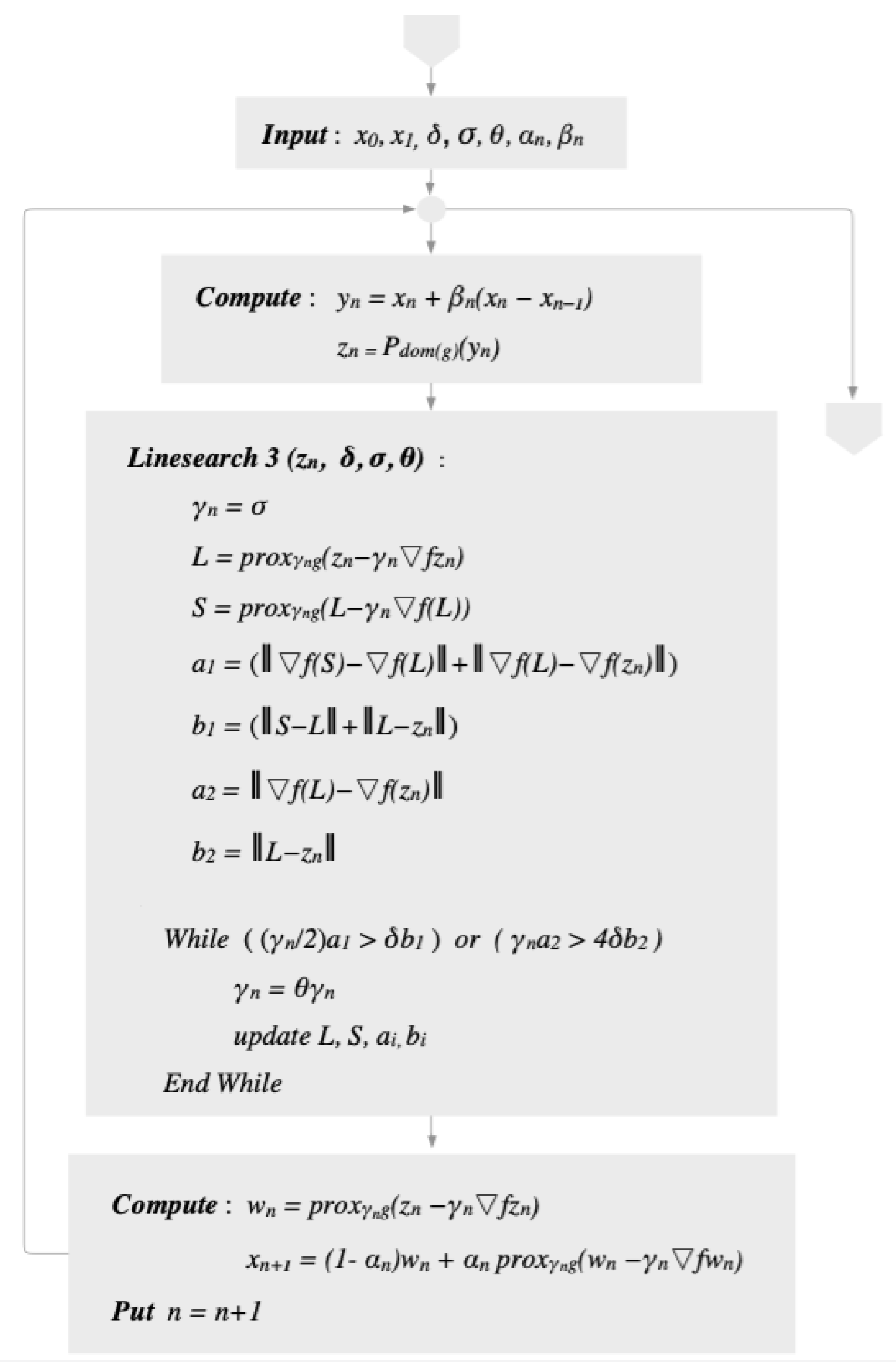
We propose a new inertial algorithm with Line Search 3 as following Algorithm 7.
| Algorithm 7. Inertial algorithm with Line Search 3. |
|
The diagram of Algorithm 7 can be seen in Figure 1.

Figure 1.
Diagram of Algorithm 7.
Next, we prove the following lemma, which will play a crucial role in our main theorems.
Lemma 8.
Let Then, for all and , the following hold:
- (I)
- (II)
where
Proof.
First, we show that is true. From (4), we know that
Moreover, it follows from the definitions of and that
for all . Consequently,
for all . It follows that
From Lemma 3, we have , and hence,
for all Then, it follows that, for any
and is proven. Next, we show . From (4), we have that
Then,
Moreover,
The above inequalities imply
for all and Hence,
Moreover, from Lemma 3, we have, for all
As a result, we obtain
for all and . Therefore,
for all and , and hence, is proven. □
Next, we prove the weak convergence result of Algorithm 7.
Theorem 9.
Let be a sequence generated by Algorithm 7. Suppose that the following hold:
- B1.
- B2.
- There exists such that for all
Then, converges weakly to some point in .
Proof.
Let ; obviously, The following are direct consequences of Lemma 8:
and
where Then, we have
Next, we show that exists. Since is nonexpansive, we have
By using Lemma 4, we have that is bounded. Consequently, and
By (10) together with Lemma 5, we conclude that exists. Since for all , we obtain
which implies that Consequently, and hence, Now, we will show that To do this, we consider the following two cases.
Case 1. , then from (9), we obtain
Therefore, we obtain from (7) that As a result, we have
Case 2. , then it follows from (9) that
It follows from (8) that and hence,
We claim that every weak-cluster point of belongs to To prove this claim, let w be a weak-cluster point of Then, there exists a subsequence of such that and hence, . Next, we show that From A2, we know that is uniformly continuous, so From (4), we also have
Hence,
By letting in the above inequality, we can conclude from (1) that and hence, It follows directly from Lemma 6 that converges weakly to a point in , and the proof is now complete. □
If we set for all in Algorithm 7, we obtain the following Algorithm 8.
| Algorithm 8. Algorithm with Line Search 3. |
|
The diagram of Algorithm 8 can be seen in Figure 2.
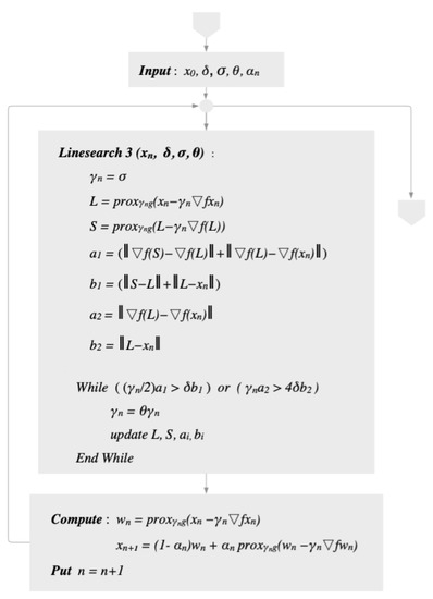
Figure 2.
Diagram of Algorithm 8.
We next prove the complexity of Algorithm 8.
Theorem 10.
Let be a sequence generated by Algorithm 8. Suppose that there exists such that for all then converges weakly to a point in In addition, if then the following also holds:
for all
Proof.
A weak convergence of is guaranteed by Theorem 9. It remains to show that (11) is true. Let and .
We first show that for all We know that in Lemma 8, so for any and , we have:
and
It follows from (14) and (17) that
respectively, for all Hence,
for all Hence, is a non-increasing sequence. Now, put in (12) and (13), then we obtain
and
Inequalities (19) and (20) imply that
for all Since we obtain
for all Summing the above inequality over we obtain
for all . Since, is a non-increasing, we have
for all . Hence,
Since is arbitrarily chosen from , we obtain
for all and the proof is now complete. □
4. Some Applications on Data Classification
In this section, we apply Algorithms 3, 5, 7, and 8 to solve some classification problems based on a learning technique called extreme learning machine (ELM) introduced by Huang et al. [28]. It is formulated as follows:
Let be a set of N samples where is an input and is a target. A simple mathematical model for the output of ELM for SLFNs with M hidden nodes and activation function G is defined by
where is the weight that connects the i-th hidden node and the input node, is the weight connecting the i-th hidden node and the output node, and is the bias. The hidden layer output matrix is defined by
The main objective of ELM is to calculate an optimal weight such that where is the training target. If the Moore–Penrose generalized inverse of exists, then is the solution. However, in general cases, may not exist or be difficult for computation. Thus, in order to avoid such difficulties, we transformed the problem into a convex minimization problem and used our proposed algorithm to find the solution without .
In machine learning, a model can be overfit in the sense that it is very accurate on a training sets, but inaccurate on a testing set. In other words, it cannot be used to predict unknown data. In order to prevent overfitting, the least absolute shrinkage and selection operator (LASSO) [29] is used. It can be formulated as follows:
where is a regularization parameter. If we set and then the problem (Section 4) is reduced to the problem (1). Hence, we can use our algorithm as a learning method to find the optimal weight and solve classification problems.
In the experiments, we aim to classify three data sets from https://archive.ics.uci.edu (accessed on 15 November 2021):
- Iris data set [30]. Each sample in this data set has four attributes, and the set contains three classes with 50 samples for each type.
- Heart disease data set [31]. This data set contains 303 samples each of which has 13 attributes. In this data set, we classified two classes of data.
- Wine data set [32]. In this data set, we classified three classes of 178 samples. Each sample contains 13 attributes.
In all experiments, we used the sigmoid as the activation function. The number of hidden nodes We calculate the accuracy of the output data by:
We chose control parameters for each algorithm as seen in Table 1.

Table 1.
Chosen parameters of each algorithm.
In our experiments, the inertial parameters for Algorithm 7 were chosen as follows:
In the first experiment, we chose the regularization parameter for all algorithms and data sets. Then, we used 10-fold cross-validation and utilized Average ACC and ERR for evaluating the performance of each algorithm.
where N is the number of folds (), is the number of data correctly predicted at fold i, and is the number of all data at fold i.
Let err = the sum of errors in all 10 training sets, err = the sum of errors in all 10 testing sets, the sum of all data in all 10 training sets, and the sum of all data in all 10 testing sets. Then,
where err = and err = .
With these evaluation tools, we obtained the results for each data set as seen in Table 2, Table 3 and Table 4.
Table 2.
The performance of each algorithm in the first experiment at the 200th iteration with 10-fold cv. on the Iris data set.
Table 3.
The performance of each algorithm in the first experiment at the 200th iteration with 10-fold cv. on the Heart disease data set.
Table 4.
The performance of each algorithm in the first experiment at the 200th iteration with 10-fold cv. on the Wine data set.
As seen in Table 2, Table 3 and Table 4, with the same regularization , Algorithms 7 and 8 perform better than Algorithms 3 and 5 in terms of accuracy, while the computation times are relatively close among the four algorithms.
In the second experiment, the regularization parameters for each algorithm and data set were chosen using 10-fold cv. We compared the error of each model and data set with various , then chose the that gives the lowest error () for the particular model and data set. Hence, the parameter varies depending on the algorithm and data set. The choice of parameters can be seen in Table 5.
Table 5.
Chosen of each algorithm.
With the chosen , we also evaluated the performance of each algorithm using 10-fold cross-validation and similar evaluation tools as in the first experiment. The results can be seen in the following Table 6, Table 7 and Table 8.
Table 6.
The performance of each algorithm in the second experiment at the 200th iteration with 10-fold cv. on the Iris data set.
Table 7.
The performance of each algorithm in the second experiment at the 200th iteration with 10-fold cv. on the Heart disease data set.
Table 8.
The performance of each algorithm in the second experiment at the 200th iteration with 10-fold cv. on the Wine data set.
With the chosen regularization parameters as in Table 5, we see that the of each algorithm in Table 6, Table 7 and Table 8 is lower than that of Table 2, Table 3 and Table 4. We can also see that Algorithms 7 and 8 perform better than Algorithms 3 and 5 in terms of accuracy in all experiments conducted.
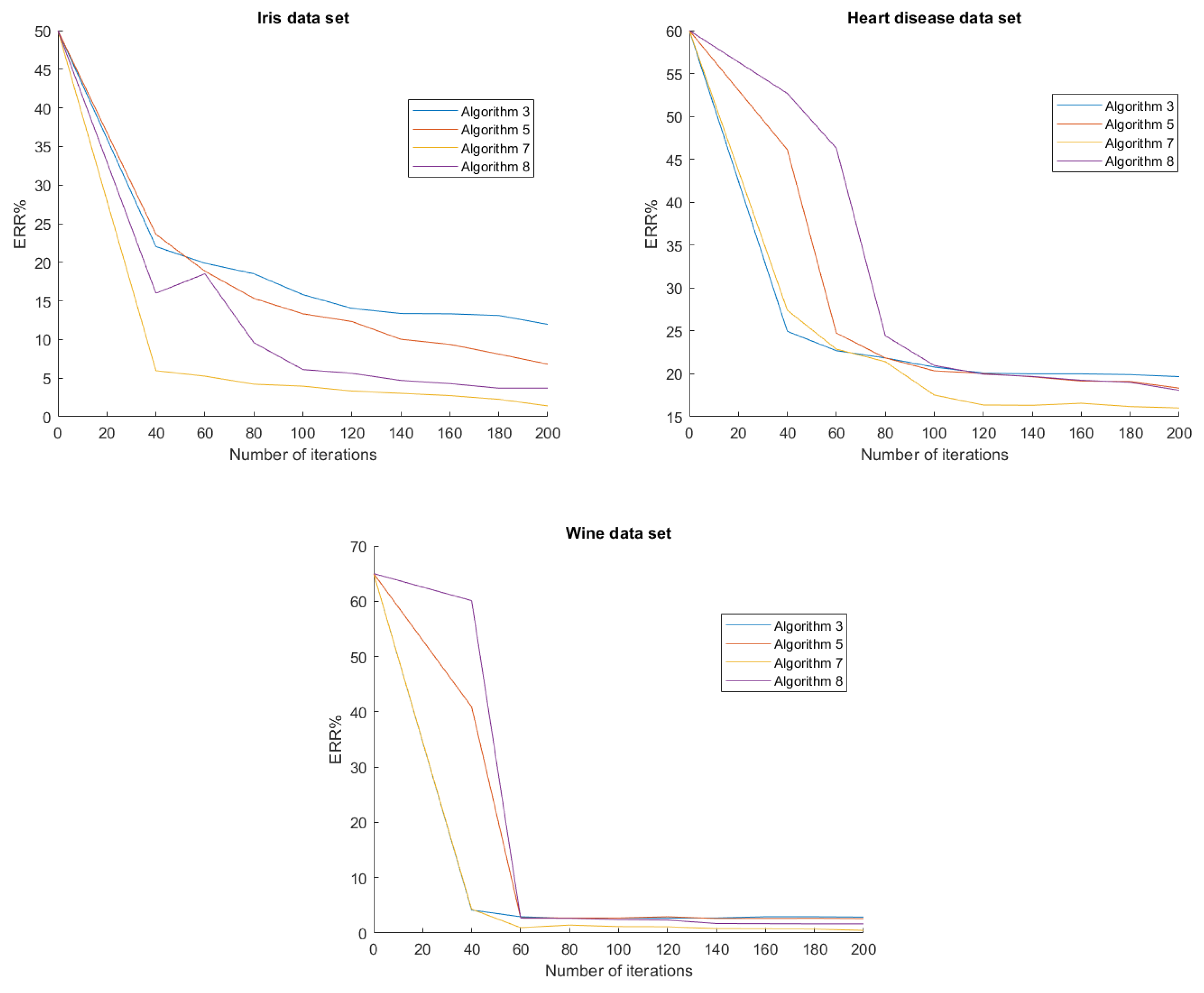
In Figure 3, we show the graph of for each algorithm of the second experiment. As we can see, Algorithms 7 and 8 have lower , which means they perform better than Algorithm 3 and 5.
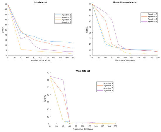
Figure 3.
ERR of each algorithm and data set of the second experiment.
From Table 6, Table 7 and Table 8, we can notice that the computational time of Algorithms 7 and 8 is slower than Algorithm 3 at the same number of iterations. However, from Figure 3, we see that at the 120th iteration, both Algorithms 7 and 8 have lower than Algorithm 3 at the 200th iteration. Therefore, the time needed for Algorithms 7 and 8 to achieve the same accuracy as or higher accuracy than Algorithm 3 is actually lower because we can compute the 120-step iteration much faster than the 200-step iteration.
5. Conclusions
We introduced a new line search technique and employed it in order to introduce new algorithms, namely Algorithms 7 and 8. Furthermore, Algorithm 7 also utilizes an inertial step to accelerate its convergence behavior. Both algorithms converge weakly to a solution of (1) without the Lipschitz assumption on . The complexity of Algorithm 8 was also analyzed and studied. Then, we applied the proposed algorithms to the data classification of the Iris, Heart disease, and Wine data set, then their performances were evaluated and compared with other line search algorithms, namely Algorithms 3 and 5. We observed from our experiments that Algorithm 7 achieved the highest accuracy in all data sets under the same number of iterations. Moreover, Algorithm 8, which is not an inertial algorithm, also performed better than Algorithms 3 and 5. Furthermore, from Figure 3, we see that at a lower number of iterations, the proposed algorithms were more accurate than the other algorithms at a higher iteration number.
Based on the experiments on various data sets, we conclude that the proposed algorithms perform better than the previously established algorithms. Therefore, for our future works, we would like to implement the proposed algorithm to predict and classify the data of patients with non-communicable diseases (NCDs) collected from Sriphat Medical Center, Faculty of Medicine, Chiang Mai University, Thailand. We aim to make an innovation for screening and preventing non-communicable diseases, which will be used in hospitals in Chiang Mai, Thailand.
Author Contributions
Writing—original draft preparation, P.S.; software and editing, D.C.; supervision, review and funding acquisition, S.S. All authors have read and agreed to the published version of the manuscript.
Funding
The NSRF via the Program Management Unit for Human Resources & Institutional Development, Research and Innovation (Grant Number B05F640183).
Data Availability Statement
All data can be obtained from https://archive.ics.uci.edu (accessed on 15 November 2021).
Acknowledgments
This research has received funding support from the NSRF via the Program Management Unit for Human Resources & Institutional Development, Research and Innovation (Grant Number B05F640183). This research was also supported by Chiang Mai University.
Conflicts of Interest
The authors declare no conflict of interest.
References
- Chen, M.; Zhang, H.; Lin, G.; Han, Q. A new local and nonlocal total variation regularization model for image denoising. Clust. Comput. 2019, 22, 7611–7627. [Google Scholar] [CrossRef]
- Combettes, P.L.; Wajs, V. Signal recovery by proximal forward–backward splitting. Multiscale Model. Simul. 2005, 4, 1168–1200. [Google Scholar] [CrossRef] [Green Version]
- Kankam, K.; Pholasa, N.; Cholamjiak, C. On convergence and complexity of the modified forward–backward method involving new line searches for convex minimization. Math. Meth. Appl. Sci. 2019, 1352–1362. [Google Scholar] [CrossRef]
- Luo, Z.Q. Applications of convex optimization in signal processing and digital communication. Math. Program. 2003, 97, 177–207. [Google Scholar] [CrossRef]
- Xiong, K.; Zhao, G.; Shi, G.; Wang, Y. A Convex Optimization Algorithm for Compressed Sensing in a Complex Domain: The Complex-Valued Split Bregman Method. Sensors 2019, 19, 4540. [Google Scholar] [CrossRef] [Green Version]
- Zhang, Y.; Li, X.; Zhao, G.; Cavalcante, C.C. Signal reconstruction of compressed sensing based on alternating direction method of multipliers. Circuits Syst. Signal Process 2020, 39, 307–323. [Google Scholar] [CrossRef]
- Hanjing, A.; Bussaban, L.; Suantai, S. The Modified Viscosity Approximation Method with Inertial Technique and Forward–Backward Algorithm for Convex Optimization Model. Mathematics 2022, 10, 1036. [Google Scholar] [CrossRef]
- Hanjing, A.; Suantai, S. A fast image restoration algorithm based on a fixed point and optimization method. Mathematics 2020, 8, 378. [Google Scholar] [CrossRef] [Green Version]
- Zhong, T. Statistical Behavior and Consistency of Classification Methods Based on Convex Risk Minimization. Ann. Stat. 2004, 32, 56–134. [Google Scholar] [CrossRef]
- Elhamifar, E.; Sapiro, G.; Yang, A.; Sasrty, S.S. A Convex Optimization Framework for Active Learning. In Proceedings of the 2013 IEEE International Conference on Computer Vision, Sydney, Australia, 1–8 December 2013; pp. 209–216. [Google Scholar] [CrossRef] [Green Version]
- Yuan, M.; Wegkamp, M. Classification Methods with Reject Option Based on Convex Risk Minimization. J. Mach. Learn. Res. 2010, 11, 111–130. [Google Scholar]
- Lions, P.L.; Mercier, B. Splitting algorithms for the sum of two nonlinear operators. SIAM J. Numer. Anal. 1979, 16, 964–979. [Google Scholar] [CrossRef]
- Polyak, B.T. Some methods of speeding up the convergence of iteration methods. USSR Comput. Math. Math. Phys. 1964, 4, 1–17. [Google Scholar] [CrossRef]
- Attouch, H.; Cabot, A. Convergence rate of a relaxed inertial proximal algorithm for convex minimization. Optimization 2019, 69, 1281–1312. [Google Scholar] [CrossRef]
- Alvarez, F.; Attouch, H. An inertial proximal method for maxi mal monotone operators via discretiza tion of a nonlinear oscillator with damping. Set-Valued Anal. 2001, 9, 3–11. [Google Scholar] [CrossRef]
- Van Hieu, D. An inertial-like proximal algorithm for equilibrium problems. Math. Meth. Oper. Res. 2018, 88, 399–415. [Google Scholar] [CrossRef]
- Chidume, C.E.; Kumam, P.; Adamu, A. A hybrid inertial algorithm for approximating solution of convex feasibility problems with applications. Fixed Point Theory Appl. 2020, 2020, 12. [Google Scholar] [CrossRef]
- Moudafi, A.; Oliny, M. Convergence of a splitting inertial proximal method for monotone operators. J. Comput. Appl. Math. 2003, 155, 447–454. [Google Scholar] [CrossRef] [Green Version]
- Sarnmeta, P.; Inthakon, W.; Chumpungam, D.; Suantai, S. On convergence and complexity analysis of an accelerated forward–backward algorithm with line search technique for convex minimization problems and applications to data prediction and classification. J. Inequal. Appl. 2021, 2021, 141. [Google Scholar] [CrossRef]
- Beck, A.; Teboulle, M. A fast iterative shrinkage–thresholding algorithm for linear inverse problems. SIAM J. Imaging Sci. 2009, 2, 183–202. [Google Scholar] [CrossRef] [Green Version]
- Boţ, R.I.; Csetnek, E.R. An inertial forward–backward-forward primal-dual splitting algorithm for solving monotone inclusion problems. Numer. Algor. 2016, 71, 519–540. [Google Scholar] [CrossRef] [Green Version]
- Verma, M.; Shukla, K.K. A new accelerated proximal gradient technique for regularized multitask learning framework. Pattern Recogn. Lett. 2017, 95, 98–103. [Google Scholar] [CrossRef]
- Bello Cruz, J.Y.; Nghia, T.T. On the convergence of the forward–backward splitting method with line searches. Optim. Methods Softw. 2016, 31, 1209–1238. [Google Scholar] [CrossRef] [Green Version]
- Burachik, R.S.; Iusem, A.N. Set-Valued Mappings and Enlargements of Monotone Operators; Springer: Berlin, Germany, 2008. [Google Scholar]
- Huang, Y.; Dong, Y. New properties of forward–backward splitting and a practical proximal-descent algorithm. Appl. Math. Comput. 2014, 237, 60–68. [Google Scholar] [CrossRef]
- Takahashi, W. Introduction to Nonlinear and Convex Analysis; Yokohama Publishers: Yokohama, Japan, 2009. [Google Scholar]
- Moudafi, A.; Al-Shemas, E. Simultaneous iterative methods for split equality problem. Trans. Math. Program. Appl. 2013, 1, 1–11. [Google Scholar]
- Huang, G.B.; Zhu, Q.Y.; Siew, C.K. Extreme learning machine: Theory and applications. Neurocomputing 2006, 70, 489–501. [Google Scholar] [CrossRef]
- Tibshirani, R. Regression shrinkage and selection via the lasso. J. R. Stat. Soc. B Methodol. 1996, 58, 267–288. [Google Scholar] [CrossRef]
- Fisher, R.A. The use of multiple measurements in taxonomic problems. Ann. Eugen. 1936, 7, 179–188. [Google Scholar] [CrossRef]
- Detrano, R.; Janosi, A.; Steinbrunn, W.; Pfisterer, M.; Schmid, J.J.; Sandhu, S.; Guppy, K.H.; Lee, S.; Froelicher, V. International application of a new probability algorithm for the diagnosis of coronary artery disease. Am. J. Cardiol. 1989, 64, 304–310. [Google Scholar] [CrossRef]
- Forina, M.; Leardi, R.; Armanino, C.; Lanteri, S. PARVUS: An Extendable Package of Programs for Data Exploration; Elsevier: Amsterdam, The Netherlands, 1988. [Google Scholar]
Publisher’s Note: MDPI stays neutral with regard to jurisdictional claims in published maps and institutional affiliations. |
© 2022 by the authors. Licensee MDPI, Basel, Switzerland. This article is an open access article distributed under the terms and conditions of the Creative Commons Attribution (CC BY) license (https://creativecommons.org/licenses/by/4.0/).