Abstract
Financial derivatives have grown in importance over the last 40 years with futures and options being actively traded on a daily basis throughout the world. The need to accurately price such financial instruments has, thus, also increased, which has given rise to several mathematical models among which is that of Black, Scholes, and Merton whose wide acceptance is partly justified by its ability to price derivatives in mature and well-developed markets. For instruments traded in emerging markets, however, the accurateness of the BSM model is unproven and new proposals need be made to face the pricing challenge. In this paper we develop a model, inspired in conformable calculus, providing greater flexibilities for these markets. After developing the theoretical aspects of the model, we present an empirical application.
MSC:
35R11; 91G20; 91G80
1. Introduction
Recent data from the Bank of International Settlements [1] reveals that the total (notional) amounts outstanding for contracts in the derivatives market was around USD 610 trillion in the first half of 2021 whereas the current world GDP is, according to Bloomberg [2], USD 84.75 billion. Since the value of financial derivatives depends on the value of the underlying financial security, pricing of such instruments is not an immediate matter. Mathematically, a model for the price of the underlying stock is needed upon which the option valuation model can be built.
This mathematical model is often taken to be the geometric Brownian motion which describes the instantaneous change in the price of the asset as the product of two factors: on the one hand, an increase proportional to opportunity cost of capital, i.e., the risk-free interest rate. On the other hand, volatile and unpredictable movements. More specifically, letting denote the price of the financial asset at time t, the model prescribes
In this equation, r is the risk-free interest rate and is the volatility. The stochastic process is assumed to be a standard Brownian motion (BM). The reader is referred to [3] for an elementary treatment oriented to financial applications, and to [4] for an in depth treatment of the mathematical aspects of this process.
Assuming that financial assets follow the geometric Brownian motion, Black, Scholes, and Merton show, in [5,6], that the price of a European option satisfies the differential equation
Since its introduction, this model has gained wide acceptance and is now a staple in option pricing. Nonetheless, several critics have arisen regarding the many assumptions founding it that question its applicability in some contexts. Among the most widely criticized aspects is the assumption that both, the underlying volatility and the risk-free interest rate are constant over time. As a response to this, several research papers, as for instance [7], have studied the BSM equation with time varying coefficients, that is, with and . Others, such as [8], have opted for maintaining constant parameters and instead interchange the Brownian motion for its fractional counterpart. In both cases, the main idea is to provide the model with more flexibility by using either parametric specification of time-varying parameters or by introducing a new relevant parameter, namely the Hurst index, to better capture the relevant features of the price dynamics.
In a similar vein, works such as [9] and, more recently, [10], have opted for changing the differential operator on the traditional BSM Equation (1) by the fractional differential operator giving rise to the so-called time fractional BSM. Due to the non-locality of the fractional derivative operator, this method serves as a tool for modelling long memory in the price dynamics. Additionally, works such as those in [11,12] develop iterative procedures to solve the BSM and the generalized fractional BSM equations using the conformable derivative operator.
In this paper, we propose a modification to BSM similar to that in [9,10], in that we change the integer-order differential operator by one of fractional order; but instead of the fractional derivative, we choose the conformable derivative operator, as in [11,12]. Furthermore, we allow for time varying parameters as in [7], thus taking advantage of two strategies simultaneously: flexibility in the parameter space and the inclusion of a new parameter (the conformable parameter) which slightly changes the dynamics of the derivative operator. Our attempt is to provide a better fit to option valuation.
Despite the abundance of alternatives for the BSM, there is not one single modification to it that has proven to be most effective and there is little, if any, empirical evidence to sustain it. In this paper, we take a step toward filling this gap. Particularly, we conduct an empirical comparison of three models: the classic BSM, the long-memory fractional BSM, and the newly proposed conformable BSM. Our findings are encouraging: The conformable BSM outperforms the other two models in most scenarios when applied in a semi-strong efficient financial market.
The remainder of the paper is structured as follows: Section 2 develops two of the most representative modifications to the BSM, namely, the time-varying parameter BSM, and the fractional BSM. We focus on the strategy followed by [7] to solve the time-varying BSM, which we later implement in the conformable case. In this section, we also introduce the conformable derivatives. In Section 3, we explicitly solve the conformable BSM equation with constant and time-varying parameters. Furthermore, we find our solution for a particular parameterization of the risk-free rate and the volatility process. The empirical analysis where the conformable BSM is compared with the two alternatives is presented in Section 4. We analyze how accurate the model is for pricing European options available in the Mexican Derivatives Market (MexDer) and find that the newly proposed model is more accurate in most cases. Finally, Section 5 presents our conclusions.
2. Previous Models and Methods
As mentioned earlier, several models have been proposed for pricing financial derivatives. Two of these models are particularly important for our proposal, namely, the BSM model with time varying parameters and the fractional BSM model. In both cases, a generalization of the traditional model is provided in an attempt to capture empirical features either of the financial market or of financial time series data. For instance, agents’ expectations can be incorporated in time-varying-parameter models whereas some theoretical economic and financial aspects have been modelled using long range dependence.
2.1. Black–Scholes–Merton with Time-Varying Parameters
The traditional BSM model of [5,6] was generalized by [7] by allowing the coefficients to be deterministic, differentiable functions of time. Such generalization intends to provide the model with the possibility of incorporating the market’s view on the behaviour of the underlying financial securities. Aided by a general transformation, the authors express the value of a European call option as the product of the BSM price, the ratio of the underlying stock prices, and a generalized discount factor.
Specifically, the authors consider the price of a call option with a strike price of K, maturity at time T, and underlying asset price process with dividend payout , risk-free interest rate and underlying volatility . Letting be such price, the authors argue that the following differential equation should be used for pricing
with terminal condition . The authors then transform the Black–Scholes PDE with time-varying parameters (2) directly into the Black–Scholes PDE with constant parameters. To this end, the price of a European call option at time with underlying equity valued under the traditional assumptions of [5,6] is denoted by . Using the transformations
and solving for , and provides the desired link between the solution to the traditional BS equation and the time-varying version, namely
where , , and are the risk-free interest rate, volatility, and strike price, respectively, for the traditional BS model of .
2.2. Standard Fractional Brownian Model
Long-range dependence has lead some authors to use the fractional Brownian motion (fBM) in asset pricing. Fractional Brownian motion is most simply described as a zero mean Gaussian process, , satisfying and for some and . Observe that for this is the standard definition of a Brownian motion. The fBM can exhibit long-range dependence in the form of a very slow decay of its autocovariance function, a feature that has attracted a lot of attention in financial mathematics. More specifically, the autocovariance function for this process is
which, depending on the value of H, may decay very slowly. There are several representations of the fBM in terms of the BM that may highlight their differences. For example, if we denote by a standard Brownian motion, choose a real number with , then we may write
where
The reader is referred to [13] or [14] for the main mathematical properties of the fBM and to [15] for a discussion on how this concept relates with the basic principles of financial theory and some possible explanations for its presence in financial data.
In [8], the authors use the standard fractional Brownian motion with a Husrt index , following the work of [16], to evaluate European options. Specifically, they model the stochastic part of asset prices with a fBM, namely, as the solution to
In a similar vein to [7] their approach, the non-fractional BSM model is adapted by a factor , making the price or the option at time t to depend on and the cost of the underlying action . However, the authors do not include time-varying parameters and, using Itô calculus, arrive at the fractional BS equation
The main strength of this model is to allow for long memory in the asset price , a feature that according to some authors is highly relevant to stochastic modelling. Additionally, the solution to this equation can be obtained by modifying the original BSM by a factor . On the other hand, long memory can be a drawback making estimation of the process a harder task and introducing a nuisance parameter, H. Additionally, no empirical evidence has been put forward to compare this model with alternative formulations.
2.3. Conformable Derivatives
Conformable derivatives are introduced in [17] by Khalil et al. These derivatives are local operators which makes them interpretable as a modification of the usual integer order derivative. Yet, conformable derivatives are not fractional derivatives which act as non-local operators and possess memory; see, for instance [18].
Fractional derivatives such as those of Caputo and Riemann–Liouville exhibit non-local memory. Indeed, by construction, fractional derivatives of f at point a are calculated on the basis of a values of the function far away from a. In a sense, we can say that these derivatives physically consider the effects that take place in such time interval. For example, the Riemann–Liouville fractional derivative of order is defined as
Thus, to compute all the information about f in the interval is to be taken in to account. As a consequence, calculation of these derivatives may be numerically challenging in practice, intensely consuming computational resources. See, for instance [17]. Additionally, fractional derivatives are often theoretically more difficult to handle than integer-order derivatives because several of the usual properties, such as the product rule or the chain rule, no longer apply.
On the opposite end, conformable derivatives do not exhibit long-range dependence or non-local memory. For instance, Ref. [17] defines the conformable derivative of order of f at t as
which satisfies the (intuitive) relation and coincides, up to a constant multiple, with the fractional derivatives of Riemann–Liouville and Caputo on polynomials. For this derivative, all the rules and properties of the integer-order derivative remain valid as can be seen, for example, in [17,18,19], which makes its computation far easier. This similarity with classic calculus has made the conformable derivative applicable in Physics [20], Engineering [21], and other sciences [22].
One advantage of the conformable derivative when compared with its fractional counterpart is that differential equations expressed in conformable derivatives are often simpler and more amenable to solution than the same equations expressed in fractional derivatives. Furthermore, conformable derivative makes it easier to introduce additional parameters into the equations without compromising the linearity of the derivative itself or of the equations in which it is used.
Particularly important in this regard is the following result, which can be found in [23] and which relates the conformable derivative of order with the classic derivative.
Theorem 1.
If a function has a conformable derivative of order and is also differentiable, then
In operator language, this means that , an equality that has been studied in [23] to assert that the conformable derivative, when applied to differentiable functions, is in fact equivalent to a change of variables, precisely .
3. Solving the BSM with Time-Varying Parameters via Conformable Calculus
In both cases, the BSM model with time-varying parameters and the Fractional Brownian model, the general solution to the relevant partial differential equation comes from a modification of the original problem which is achieved by using a transformation of coordinates, a change of variables. As explained in the previous section, the conformable derivative can also be seen as a change of variables in classic calculus. Therefore, it is plausible that using the conformable derivative in the BSM model will provide new insights.
In this section, we solve the BSM equation with time varying parameters using conformable calculus. Our reference model is that of [7] and the rules of the conformable derivative follow those explained by [23]. Whereas classic derivatives measure the rate of change of a function in the vicinity of a given point and, thus, approximate it, conformable derivatives provide non-linear approximations to the same function. In fact, Theorem 4.1 in [19] provides a Taylor-series expansion for infinitely -differentiable functions.
The idea of using a time varying BSM and conformable calculus is, thus, an effort to include more complex dynamics that are possible with the traditional model without making resource of long-memory processes or derivatives. Let, thus, be the price at time t of an equity, and let be the price at time of a European call option expiring at time T with strike price . Assume also that the risk-free interest rate and the volatility of the underlying equity are time-dependent and denote them by and , respectively. The theory developed by [6] implies that the value process satisfies the partial differential Equation (2).
In order to study this equation using the conformable derivative, we assume that derivatives are taken conformably in S, that is we interchange the operator with . To express Equation (2) in this new derivative, we begin by using the change of variables and express
We then compute the second –derivative of this expression and obtain the Conformable Black–Scholes equation
When the coefficients are fixed, the change of variables allows for a solution of (4) very much as in the traditional case of [5,6], namely:
To solve the conformable Black–Scholes equation with time-varying parameters, namely
We follow [7] and apply the relations (3) to (5) to make its parameters constant functions of time. This leads, after some algebra, to the following relations
Grouping and integrating these equations leads to
Continuing our calculations as in [7], we obtain , and . So far, this is a completely abstract result in that it allow for any form of time-dependence in the parameters and . To make this result applicable, we need to determine an structure for these functions. An empirical analysis suggests that using order-two polynomials is suitable for representing both, volatility and risk-free interest rates, in the short term. We thus use and .
Using the quadratic representations of the risk-free interest rate and the volatility, we can solve explicitly for the unknowns and the transforming functions obtaining
These expressions yield the value of the European call option as
Thus, the solution to the conformable Black–Scholes equation with time-varying coefficients is given by
with the solution corresponding to the constant parameter case in (3).
4. Empirical Analysis
Although many modifications to the BSM model have been produced, few are the papers in which the empirical viability of the proposed solution is tested. It is well known, as can be seen for example in [24], that the BSM model, despite its simplifying assumptions, is a useful valuation tool. Nonetheless, the relative appropriateness of the model may not be ubiquitous and may fail, specially in scarcely developed financial markets.
We consider a sample of 16 European call options on stocks that were listed on the Mexican Derivatives Market (MexDer) on 3 November 2020 and which are listed in Table 1. According to MexDer, in the Bulletin entitled “General Conditions of Contracting of the Contracts of Options on Shares”, each time an issue of options is made, the shares on which the contracts will be signed are published five working days in advance of the price negotiation date. To obtain the final value of the contract, MexDer takes the closing price of the underlying asset and the working price shall be equivalent to the last price of the contract at the working day immediately preceding the trading. The initial worth of the bid is set by using the traditional BSM of [5,6]. Almost needless to mention, all the stocks upon which financial options are sold must be listed on the Mexican Stock Exchange.

Table 1.
Stocks considered for the European call options.
For each option, we consider the five different prices available on the Bloomberg terminal for the maturities of 17, 45, 136, and 277 days. Our data span the period starting on 2 January 2017 and ending on 3 November 2020. We collected the data of the price per share of each firm and use the 28-days government treasury bonds (Cetes) yield as our risk-free interest rate. In order to estimate the second degree polynomials that best represent the volatility and the risk-free interest rate we follow a two step procedure:
- First, we estimate the GJR-GARCH (1, 1) process of [25] with skewed t innovations to each of the underlying assets;
- We then fit a quadratic regression to the estimated volatility process and use these coefficients to solve the conformable Black–Scholes equation with time-varying parameters.
More precisely, we consider the log-returns of each asset defined as as is usual in empirical finance. See for instance [26,27] or [28]. We estimate the model
by maximum likelihood using the rugarch package [29] of the R language for statistical computing [30]. As a result of this estimation procedure, we obtain, for each asset, the estimated volatility process . Letting denote the risk-free interest rate, we then use OLS to estimate
For this to make sense, we first test for the presence of ARCH effects using the Lagrange multiplier test of [31] in each of the series. All the series reject the null of no ARCH effects at the 1% significance level with p-values ranging from to . Having established the existence of ARCH effects, despite the semi-strong efficiency of the market, we estimate the same model for each series. Traditionally, on econometric or time series settings, several goodness of fit tests are conducted to each series to assess the fit of the proposed model. So, for instance, the statistical significance of the coefficients is checked and the model is re-estimated as needed to exclude insignificant parameters. Additionally, diagnostic tests, such as the (Negative or Positive) Sign-Bias, stability diagnostics (such as Nyblom’s test), etc., are used until a “best model” is sequentially built for each series. See, for example [32] and the references therein.
The main aim of this econometric exercise is to capture all the relevant features of a time series in order to either explain it or forecast it and to draw inferences on important relations between series. However, our aim is different. We only estimate the GJR-GARCH process in order to obtain an estimate of the conditional variance process . For this estimate to be a reasonable approximation to the underlying variance, it is only necessary that the parameter estimation be consistent and the model be general enough to encompass different alternative behaviours for the modelled series. It is in this search for flexibility that we choose the GJR-GARCH process, which contains the classic, symmetric GARCH process as a particular case, as a base model for all the series. The main point to make here is that even if the underlying series does not display asymmetric features (and, thus, fails the sign-bias tests); but the parameter estimation remains consistent, the estimate of the underlying variance will vary only very slightly. Furthermore, it is also common practice to check for the distributional assumptions of the model. In our case, we are assuming a skewed t distribution which may fit some series and not fit others. Nonetheless, in the cases in which this distribution does not fit, the estimation becomes a quasi-maximum-likelihood estimation procedure which, in most cases, also yields consistent estimates of the parameters and, consequently, of the variance process.
As an illustration of these features, we consider Grupo México for which the ARCH test reports a p-value of solidly rejecting the absence of heteroscedasticity. Fitting the GJR-GARCH, we obtain a p-value of 0.7664 for the Sign-Bias test, 0.5741 for the Negative Sign-Bias test, 0.4870 for the Positive Sign-Bias test and, finally, 0.6880 for the Joint Effect Sign-Bias test. All these results indicate that the series is actually better modelled by a symmetric GARCH process, from an econometric standpoint. Nonetheless, the quasi-maximum-likelihood estimation being consistent, the estimated variances are virtually indistinguishable. Figure 1 shows the estimated variances under two models: The GJR-GARCH with skewed t innovations and the simple GARCH model with normally distributed errors. All diagnostics point to the second as the better model.
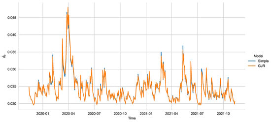
Figure 1.
Variance process as estimated from two specifications: the GJR-GARCH with skewed t innovations and the simple GARCH model with normally distributed errors. Despite all diagnostics pointing to the second model, the estimated variance processes are indistinguishable.
Once the GJR-GARCH model and the polynomial trend are estimated, we solve the conformable BS Equation (5) using the volatility and risk-free interest rate predicted by this model. In order to establish a meaningful comparison with other models, we also consider the classic BSM model and the model based on the Fractional Brownian motion. We estimate the conformability parameter by optimizing the fit on the price, that is, by solving the problem
where is the price of the call predicted by the model in (5) with conformable parameter and is the observed price. We solve an analogous problem for estimating the Hurst index H.
Table 2 shows basic information on the firms selected including its GICS classification (using only Industry and Sector), the stock price on expiration date, the range of prices for the call option, the market implicit volatility, and the stationary volatility as estimated by the GJR-GARCH(1, 1) process.
Table 2.
Descriptive facts and volatility statistics for each firm.
Figure 2 depicts the errors of each model for all the firms included in the study faceted by the time to maturity of the options. The blue and orange line share the left-hand vertical axis whereas the olive line is indexed to the right-hand y axis. As can be easily seen, the axes have very different scales in all cases, which immediately shows that the conformable BSM model is more flexible than the classical alternatives and produces a more accurate valuation. Furthermore, there does not appear to be any systematic pattern of under or over-valuation by the conformal BSM.
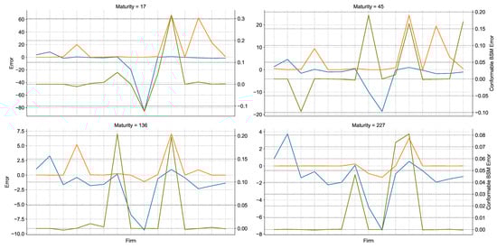
Figure 2.
Percentage error for each firm (x axis), model and contract. The blue lines corresponds to the Black–Scholes model, the orange line to the Fractional Black–Scholes, and the olive line to the conformable Black–Scholes whose scaled is signalled on the right axis or each plot.
The cases in which the conformal BSM model errs the most all seem to share a common feature, namely, that the price of the underlying asset differs widely from that of the option under valuation. Even in these cases, the conformal BSM is rarely outperformed by either the BSM or the fractional BSM. This inaccuracy is, however, to be expected since a larger spread between the current stock price and the call option implies the expectations of the investors come into play importantly and this speculative behaviour is not captured by the historical volatility process.
Table 3 shows the mean, median, and maximum value attained by the errors in the different models. In this table, all four maturities are summarized together. As can be seen, the magnitude of the errors is much smaller in the conformal BSM model consistently throughout all the firms included in the study. This is certainly a consequence of the flexibility offered by the conformable parameter and the consequent non-linear local approximation to the value of the option that the CBSM model implicitly does.
Table 3.
Aggregate measures of error over all maturity dates for each firm and model.
Figure 3 shows the dispersion of the estimated values for the conformable parameter grouped by Industry. Notably, higher maturities imply less dispersion in the estimate which is heteroskedastic in Industry. More specifically, Consumer Staples, Materials, and Industrial sectors present the highest variability overall, whereas Communication Services is the most variable for longer maturities. Note also that the value of is mostly close to 1, in which case the conformable BSM model is the classic BSM. It is important to emphasize that the conformal BSM worked best for firms and maturities with between 0.75 and 0.96, suggesting that only a slight deviation from the classical BSM is necessary to significantly improve the fit.
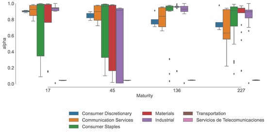
Figure 3.
Distribution of the value of among all five exercise prices for the options by Industry.
5. Conclusions
Our empirical analysis suggests that the conformable Black–Scholes–Merton model may provide a superior fit for valuing European call options when compared to both, the classical BSM and the fractional BSM model. In fact, out of all the scenarios in which the model was tested, it provided the best fit in over 90% of the cases. It should be stressed that our appreciation of these advantages is only preliminary. Indeed, establishing them more fully and generally, would require a more robust statistical procedure which we leave as an open question for future research.
Another aspect that could be of interest in asset pricing models is that of transaction costs. In our model, these costs are not considered explicitly; but the goodness of fit that is observed suggests that the flexibility implied by the use of the conformable derivative operator may capture, at least partially, such effects.
This improved fit comes from the model’s ability to better adjust locally to the value surface by allowing some curvature in its approximation. This curvature is itself induced by the power terms of the form which appear in the conformable BS Equation (5). As was discussed earlier, values of the conformable parameter in the vicinity of seem to perform in most cases, although there is some variability present.
Interestingly enough, it seems that the only discernible circumstance under which the model failed is that of strongly speculative options, that is, options whose strike price differs widely from that of the underlying stock. In these cases, however, most models based on past behaviour will also fail, a feature that is illustrated by the failure of the GJR-GARCH model to capture the implicit volatility for such stock.
It should be stressed that the Mexican Financial Market is not a fully developed market in which ownership of public firms is widely spread. Indeed, the 2021 Financial Yearbook, published by Bolsa Mexicana de Valores (BMV) states that around 53% of the non-financial public firms are managed either by the owner or by a close relative whereas 19% are owned and directed by the same person. Thus, in up to 72% of this public firms there is not a real and deep distinction between managerial and stockholders interests. Furthermore, organized crime, violence, and insecurity, together with the recent economic crisis accentuate the lack of interrelationship between firms and financial institutions which make the Mexican financial market semi-strong in terms of its efficiency. This lack of development is, most likely, one reason why the traditional models do not provide a better fit to option pricing.
Importantly, whereas some research has been conducted on applying conformable calculus to solve the BSM equation, the authors usually reason by homotopy without analyzing the dynamics of the underlying asset. In contrast, we modify the BSM equation using the conformable derivative operator precisely in the underlying asset. Furthermore, this is the first study, to our knowledge, to present an empirical application of the results and a practical comparison between different models.
Author Contributions
Conceptualization, G.F.-A. and N.M.; methodology, N.M. and P.M.-B.; software, P.M.-B.; validation, G.F.-A. and N.M.; formal analysis, G.F.-A., N.M., P.M.-B.; investigation, P.M.-B.; resources, N.M. and P.M.-B.; data curation, P.M.-B.; writing—original draft preparation, P.M.-B.; writing—review and editing, N.M.; visualization, P.M.-B. and N.M.; supervision, G.F.-A. and N.M.; project administration, G.F.-A.; funding acquisition, P.M.-B. All authors have read and agreed to the published version of the manuscript.
Funding
This research was funded by Universidad Iberoamericana Ciudad de México.
Data Availability Statement
The stock prices and risk-free interest rate Cetes can be found at finance.yahoo.com (accessed on 23 March 2022). For the option prices, the authors made resource of the Bloomberg terminal and the generated datasets are available upon request.
Conflicts of Interest
The authors declare no conflict of interest.
Abbreviations
The following abbreviations are used in this manuscript:
| BMS | Black–Scholes–Merton |
| fBMS | Fractional Black–Scholes–Merton |
| CBMS | Conformable Black–Scholes–Merton |
References
- Exchange-Traded Derivatives Statistics. Available online: https://www.bis.org/statistics/extderiv.htm (accessed on 18 April 2022).
- World GDP. Bloomberg Terminal. Available online: https://bba.bloomberg.net/?utm_source=bloomberg-menu&utm_medium=company (accessed on 18 April 2022).
- Mikosch, T. Elementary Stochastic Calculus with Finance in View; Advanced Series in Statistical Science & Applied Probability; World Scientific: Singapore, 1998; Volume 6. [Google Scholar]
- Karatzas, I.; Shreve, S.E. Brownian Motion and Stochastic Calculus; Springer: New York, NY, USA, 1988. [Google Scholar]
- Black, F.; Scholes, M. The Pricing of Options and Corporate Liabilities. J. Political Econ. 1973, 81, 637–654. [Google Scholar] [CrossRef]
- Merton, R.C. Theory of Rational Option Pricing. Bell J. Econ. 1973, 4, 141–183. [Google Scholar] [CrossRef]
- Rodrigo, M.R.; Mamon, R.S. An alternative approach to solving the Black–Scholes equation with time-varying parameters. Appl. Math. Lett. 2006, 19, 398–402. [Google Scholar] [CrossRef]
- Njomen, D.A.N.; Djeutcha, E. Solving Black-Schole Equation Using Standard Fractional Brownian Motion. J. Math. Res. 2019, 11, 142–157. [Google Scholar] [CrossRef]
- Wyss, W. The fractional Black–Scholes equation. Fract. Calc. Appl. Anal. Int. J. Theory Appl. 2000, 1, 51–61. [Google Scholar]
- Zhang, H.; Liu, F.; Turner, I.; Yang, Q. Numerical solution of the time fractional Black–Scholes model governing European options. Comput. Math. Appl. 2016, 71, 1772–1783. [Google Scholar] [CrossRef]
- Yavuz, M. Novel solution methods for initial boundary value problems of fractional order with conformable differentiation. Int. J. Optim. Control. Theor. Appl. 2018, 8, 1. [Google Scholar] [CrossRef]
- Yavuz, M.; Özdemir, N. A different approach to the European option pricing model with new fractional operator. Math. Model. Nat. Phenom. 2018, 13, 12. [Google Scholar] [CrossRef]
- Samorodnitsky, G. Long Range Dependence. Found. Trends® Stoch. Syst. 2007, 1, 163–257. [Google Scholar] [CrossRef]
- Biagini, F.; Hu, Y.; Øksendal, B.; Zhang, T. Stochastic Calculus for Fractional Brownian Motion and Applications; Springer: London, UK, 2008. [Google Scholar]
- Cont, R. Long range dependence in financial markets. In Fractals in Engineering; Springer: London, UK, 2005. [Google Scholar]
- Necula, C. Option Pricing in a Fractional Brownian Motion Environment; Advances in Economic and Financial Research—DOFIN Working Paper Series 2; Bucharest University of Economics, Center for Advanced Research in Finance and Banking—CARFIB: Bucharest, Romania, 2008. [Google Scholar]
- Khalil, R.; Al Horani, M.; Yousef, A.; Sababheh, M. A new definition of fractional derivative. J. Comput. Appl. Math. 2014, 264, 65–70. [Google Scholar] [CrossRef]
- Kilbas, A.A.; Srivastava, H.M.; Trujillo, J.J. Theory and Applications of Fractional Differential Equations; Volume 204 (North-Holland Mathematics Studies); Elsevier Science Inc.: Cambridge, MA, USA, 2006. [Google Scholar]
- Abdeljawad, T. On conformable fractional calculus. J. Comput. Appl. Math. 2015, 279, 57–66. [Google Scholar] [CrossRef]
- Cao, Y.; Parvaneh, F.; Alamri, S.; Rajhi, A.A.; Anqi, A.E. Some exact wave solutions to a variety of the Schrödinger equation with two nonlinearity laws and conformable derivative. Results Phys. 2021, 31, 104929. [Google Scholar] [CrossRef]
- Mayo-Maldonado, J.C.; Fernandez-Anaya, G.; Ruiz-Martinez, O. Stability of conformable linear differential systems: A behavioural framework with applications in fractional-order control. IET Control. Theory Appl. 2020, 14, 2900–2913. [Google Scholar] [CrossRef]
- Di Crescenzo, A.; Kaabar, M.K.A.; Martínez, F.; Martínez, I.; Siri, Z.; Paredes, S. Novel Investigation of Multivariable Conformable Calculus for Modeling Scientific Phenomena. J. Math. 2021, 2021, 3670176. [Google Scholar] [CrossRef]
- Anderson, D.; Camrud, E.; Ulness, D. On the nature of the Conformable derivative and its applications to Physics. J. Fract. Calc. Appl. 2019, 10, 92–135. [Google Scholar]
- Hull, J. Options, Futures, and Other Derivatives, 6th ed.; Pearson Prentice Hall: Upper Saddle River, NJ, USA, 2006. [Google Scholar]
- Glosten, L.R.; Jagannathan, R.; Runkle, D.E. On the relation between the expected value and the volatility of the nominal excess return on stocks. J. Financ. 1993, 48, 1179–1801. [Google Scholar] [CrossRef]
- Cont, R. Empirical properties of asset returns: Stylized facts and statistical issues. Quant. Financ. 2001, 1, 223–236. [Google Scholar] [CrossRef]
- Tsay, R. Analysis of Financial Time Series; Wiley: Hoboken, NJ, USA, 2005. [Google Scholar]
- Campbell, J.Y.; Lo, A.W.; MacKinlay, A.C. The Econometrics of Financial Markets; Princeton University Press: Princeton, NJ, USA, 1997. [Google Scholar]
- Ghalanos, A. Rugarch: Univariate GARCH Models, R Package Version 1.4-7. 2022.
- R Core Team. R: A Language and Environment for Statistical Computing; R Foundation for Statistical Computing: Vienna, Austria, 2021. [Google Scholar]
- Engle, R.F. Autoregressive Conditional Heteroscedasticity with Estimates of the Variance of United Kingdom Inflation. Econometrica 1982, 50, 987–1007. [Google Scholar] [CrossRef]
- Franq, C.; Zakoïan, J.M. GARCH Models: Structure, Statistical Inference and Financial Applications, 1st ed.; Wiley: Hoboken, NJ, USA, 2010. [Google Scholar]


Publisher’s Note: MDPI stays neutral with regard to jurisdictional claims in published maps and institutional affiliations. |
© 2022 by the authors. Licensee MDPI, Basel, Switzerland. This article is an open access article distributed under the terms and conditions of the Creative Commons Attribution (CC BY) license (https://creativecommons.org/licenses/by/4.0/).