1. Introduction
In the year 1650, Pietro Mengoli posed a mathematical problem, which is now known as the Basel Problem. Its solution was achieved nearly 85 years later, in 1735 by Leonard Euler [
1], who used Taylor’s series of sine functions in an ingenious way and then generalised the formula for all real powers greater than 1. The approach, however, to implementing a fundamental theorem of algebra (which is for finite zeros) on an infinite polynomial (with infinite zeros) was based on Euler’s intuition and remained unproved for another century, when in the early 1800s, Wierstrass gave a validation of Euler’s work using the so-called Weierstrass factorisation theorem. Following these findings, in 1859, nearly two centuries after Mengoli’s work, Bernard Riemann extended the formula defined by Euler to the domain of complex numbers with the motivation to find a relation between zeros of the function and the distribution of prime numbers.
The slow progress in the development of this field over the first two centuries suddenly surged after Riemann’s study displayed the (zeta) function’s relation with the prime counting function. Over the next two centuries, researchers discovered that not only is the zeta function crucial in understanding the distribution of prime numbers but also the function and its generalisations have many direct or indirect applications in many advanced fields such as cryptography (applications of prime number theory), cosmology [
2], quantum field theory [
3,
4] and string theory [
5].
Due to such impactful applications, researchers have studied different infinite series and zeta functions in depth [
6,
7,
8,
9,
10] over the past few decades. Coffey [
6] obtained a faster convergent series representation of the Hurwitz zeta function, whereas Kanemitus et al. [
7] provided integral representations and gave proofs of certain available results, including the Ramanujan formula. Vepštas [
8] provided a technique to obtain faster convergence of oscillatory sequences and applied them to Hurwitz zeta functions and polylogarithms. Nisar [
9] generalised the Hurwitz–Lerch zeta function of two variables. Riguidel [
10] utilised the computational approach to propose the morphogenic interpretation of Riemann zeta function.
Moreover, as we showcased in Part I [
11], the floor–ceiling and ceiling–floor theorems allow researchers to derive, study and analyse new results, and corresponding novel real-life applications can be found with the emergence of such results.
Hence, continuing the study in a similar direction, in this part, we attempted to generalise different infinite series and zeta functions (such as geometric series, Hurwitz zeta function, and polylogarithms) using the theorems developed in Part I [
11].
Outline of the Article
Section 2 contains the preliminary results that are utilised in our study.
Section 3 provides the cases for
for the floor–ceiling theorem and the ceiling–floor theorem of Part I [
11]. These cases provide foundations for the results obtained in
Section 4,
Section 5 and
Section 6.
Section 7 specifically presents the corollaries of the results proved in the previous three sections. In
Section 8, some of the zeros of newly developed zeta functions are given and their behaviours are discussed in a bounded interval using domain colouring.
Section 9 gives the results on particular values.
Section 10 provides some miscellaneous results.
Section 11 discusses the scope for further studies, and finally,
Section 12 concludes the work conducted in this pair of articles.
2. Preliminaries
The following results and definitions are useful for our study:
2.1. Hurwitz Zeta Function
The Hurwitz zeta function [
3]
is a function of complex variables
s and
t defined as an infinite sum:
The series is absolutely convergent for all complex values of s and t when and .
2.2. Polylogarithm
The polylogarithm function [
12] is an infinite series of the following form:
where
.
2.3. Riemann Zeta Function
The Riemann zeta function [
5]
is a function of the complex variable
s defined as an infinite sum:
The function converges for all complex values of
s when
and is defined as
2.4. Fibonacci Numbers and Reciprocal Fibonacci Constant
The
nth Fibonacci number [
13] is given by the following formula:
Furthermore, a series of reciprocals of all Fibonacci numbers gives a constant (irrational) value:
where
is the reciprocal Fibonacci constant.
2.5. Floor and Ceiling Functions
The floor function [
14] of any real number
x (denoted by
) gives the greatest integer not greater than
x, i.e.,
. For example,
and
.
The ceiling function [
14] (denoted by
) similarly gives the smallest integer not smaller than
x, i.e.,
. For example,
and
.
From the above, we can see that if and only if .
3. Foundations
3.1. Floor–Ceiling Theorem
Theorem 1. Let , and let be any sequence and let corresponding series be convergent; then, the following equalities hold true.or alternatively, Proof. We have ([
11], Section 3, Equation (12))
Now, the following observation can be easily made:
Hence, by applying limit
, the previous equation reduces to Equation (
5).
Furthermore, consider the right-hand side of Equation (
5):
which is the right-hand side of Equation (
6). □
3.2. Ceiling–Floor Theorem
Theorem 2. Let , let be any sequence and let corresponding series be convergent; then, the following equalities hold true.or alternatively, Proof. We have ([
11], Section 3, Equation (16))
Now, the following observation can be easily made:
Hence, by applying limit
, the previous equation reduces to Equation (
7).
Furthermore, consider the right-hand side of Equation (
7):
which is the right-hand side of Equation (
8). □
4. ‘F’ and ‘C’ Generalised Functions
4.1. Definitions
In order to avoid misunderstanding our new results with the available definitions, we assign ’F’ or ’C’ (representing use of floor and ceiling functions, respectively) prefixes to all of the available definitions.
For example, the F-Hurwitz zeta function can be defined as the following equation:
whereas the C-Riemann zeta function is defined as the following equation:
Using the same analogy, the C-Hurwitz zeta function, F-polylogarithm, C-polylogarithm and F-Riemann zeta function can also be defined.
Furthermore, by implementing floor and ceiling functions, any available infinite series can be generalised as ‘F’ or ‘C’ series (i.e., For Lerch zeta function, the corresponding F-Lerch and C-Lerch zeta functions can be defined).
4.2. Theorems
For each ‘F’ and ‘C’ generalised series, a corresponding theorem can be provided and proved, which relate them to an equivalent series (which is due to Theorem 1 or Theorem 2).
Take the F-Hurwitz zeta function and the C-polylogarithm for example:
Theorem 3. (F-Hurwitz Zeta Function)
The series has an equivalent form, given below: Proof. Equation (
9) can be obtained by substituting
and
in Equation (
5). □
Theorem 4. (C-Polylogarithm)
The series has an equivalent form, given below: Proof. Equation (
10) can be obtained by substituting
and
in Equation (
7). □
Remark 1. Every series or function available in the literature can be generalised using the same analogy. However, to avoid repetition, we have provided just a couple of examples to depict the scope of Theorems 1 and 2 (the general rule for the notation is and for ‘F’ and ‘C’ generalised functions, respectively, where is the notation for the regular definition of the same function).
5. Generalised Geometric Series
5.1. Floor Geometric Series
Theorem 5. Let and , then the following equation holds true. Proof. Substituting
and
in Equation (
6), we have
Furthermore, with basic manipulations, we arrive at Equation (
11). □
5.2. Ceiling Geometric Series
Theorem 6. Let and ; then, following equation holds true. Proof. Substituting
and
in Equation (
8), we have
Furthermore, with basic manipulations, we arrive at Equation (
12). □
6. Generalised Reciprocal Fibonacci Series
6.1. Shah–Pingala Function
Definition 1. For , we define the Shah–Pingala function using the following equation:where is the nth Fibonacci number (Section 2.4). The reciprocal Fibonacci constant is a special case of the new definition for .
Theorem 7. Shah–Pingala function converges for all .
Proof. The
nth term is
. We know that
We also know that
for
. Hence,
Therefore, the necessary condition holds.
Furthermore, considering the ratio test for series convergence, we have
Since the limit , the series converges. □
6.2. Floor Reciprocal Fibonacci Function
Theorem 8. Let , and let be Fibonacci sequence; then, Proof. Substituting
and
in Equation (
5), we obtain Equation (
14). □
6.3. Ceiling Reciprocal Fibonacci Function
Theorem 9. Let , and let be Fibonacci sequence; then, Proof. Substituting
and
in Equation (
7), we obtain Equation (
15). □
7. Corollaries
7.1. Corollaries of ‘F’ and ‘C’ Generalised Functions
Corollary 1. (F-Shah–Hurwitz Zeta Function)
For the F-Shah–Hurwitz zeta function (a special case of the F-Hurwitz zeta function at ) and the Hurwitz zeta function , the following equation holds true.or alternatively,where Given the analytic continuation of the Hurwitz zeta function, we observe that can be defined for , and hence, can be defined such that .
Proof. Substituting
and
, we obtain
Considering the right-hand side of the previous equation, we have
Finally, the alternate (integral representation) form of the equation can be obtained by substituting
(from Equation (
1)). □
Corollary 2. (C-Shah–Hurwitz zeta function)
For the C-Shah–Hurwitz zeta function (a special case of the C-Hurwitz zeta function at ) and the Hurwitz zeta function , the following equation holds true.or alternatively,where Given the analytic continuation of the Hurwitz zeta function, we observe that can be defined even for , and hence, can be defined such that .
Proof. Substituting
and
, we have
Consider the right-hand side of the previous equation:
Finally, the alternate (integral representation) form of the equation can be obtained by substituting
(from Equation (
1)). □
Corollary 3. (F-Shah–Riemann Zeta Function)
For any a of the form and , the following equation holds true.or alternatively, Furthermore, given the analytic continuation of the Riemann zeta function, we observe that can be defined for , and hence, can be defined such that .
Proof. Equation (
20) can be obtained by substituting
in Equation (
16). Moreover, we may consider an integral representation of the Riemann zeta function from Equation (
3) to obtain Equation (
21). □
Corollary 4. (C-Shah–Riemann Zeta Function)
For any a of the form and , the following equation holds true.or alternatively, Again, given the analytic continuation of the Riemann zeta function, we observe that can be defined even for , and hence, can be define such that .
Proof. Equation (
22) can be obtained by substituting
in Equation (
18). Moreover, we may take an integral representation of the Riemann zeta function from Equation (
3) to obtain Equation (
23). □
Remark 2. All of the series in Corollaries 1–4 have poles at , but the following can be simply observed for :and This shows that, even if the set of two series may individually have poles at , their difference is convergent for .
Remark 3. The analogy used in Corollaries 1–4 can be implemented to different functions such as the Lerch zeta function. 7.2. Corollaries of Generalised Geometric Series
Corollary 5. For , polylogarithm and any , the following equation holds true. Proof. Equation (
26) can be obtained by substituting
in Equation (
11). □
Corollary 6. For , polylogarithm and any , the following equation holds true. Proof. Equation (
27) can be obtained by substituting
in Equation (
12). □
7.3. Corollaries of Generalised Reciprocal Fibonacci Series
Corollary 7. Let be Fibonacci sequence, , and let denote a Shah–Pingala function; then, the following equation holds true. Proof. Equation (
28) can be obtained by substituting
in Equation (
14). □
Corollary 8. Let be Fibonacci sequence, , and let denote the Shah–Pingala function; then, the following equation holds true. Proof. Equation (
29) can be obtained by substituting
in Equation (
15). □
8. Plots and Zeros: F-Shah–Riemann Zeta and C-Shah–Riemann Zeta Functions
For this study, we consider all of the available zeros of Riemann zeta functions, i.e., the real zeros and the known complex zeros on the critical strip , as trivial solutions (already available zeros). Keeping that in view, we consider the negative solutions and the solutions in which the imaginary parts are in the radius (imaginary part of solutions of the Riemann zeta function) as trivial for the new zeta functions. Moreover, positive real zeros and the solutions in which imaginary parts are not in the radius are considered non-trivial zeros. In all six of the plots, we focused on the behaviour of the functions near their non-trivial zeros.
8.1. Zeros of F-Shah–Riemann Zeta Function
In this subsection, utilising the right-hand side of the Equation (
20), we obtain the solutions (given in
Table 1) of the F-Shah–Riemann zeta function. Furthermore, we give three
Figure 1,
Figure 2 and
Figure 3, and they are plotted in the intervals of the non-trivial (positive real) zeros and the poles of F-Shah–Riemann zeta function for
,
, and
, respectively.
The function has q poles, positive real zeros (non-trivial zeros) and infinite negative real zeros (each zero corresponding to each negative even integer).
The complex zeros are achieved by implementing the Newton–Raphson method at point for different available values of t.
8.2. Zeros of C-Shah–Riemann Zeta Function
In this subsection, utilising the right-hand side of Equation (
22), we obtain the solutions (given in
Table 2) of the C-Shah–Riemann zeta function. Furthermore, we give three
Figure 4,
Figure 5 and
Figure 6, and they are plotted in the intervals of the non-trivial (positive real) zeros and the poles of F-Shah–Riemann zeta function for
,
and
, respectively.
The function has q poles, pairs of non-trivial of complex zeros ( zeros), which were observed in the plots. There are infinite real zeros (each zero corresponds to each negative even integer) with no non-trivial (positive) real zero.
The trivial complex zeros are achieved by implementing the Newton–Raphson method with an initial guess for different available values of t, whereas the non trivial complex zeros are obtained by considering an initial guess in the converging region of the plot (for example, we considered for the C-Shah–Riemann zeta function for ).
9. Results for Specific Values
9.1. Specific Values—‘F’ and ‘C’ Generalised Functions
For
, ‘
F’ and ‘
C’ generalised series reduce to the original series (consider the F-Hurwitz zeta function and C-Riemann zeta, for example).
9.2. Specific Values—Generalised Geometric Series
Substituting
in Equation (
11), we obtain
or substituting
in Equation (
12), we obtain
both of which hold true.
9.3. Specific Values—Generalised Reciprocal Fibonacci Series
For
in Equations (
14) and (
15), we have
.
10. Miscellaneous Results
Let the two functions be defined as
and
, which yield the number of repetitions of
and
, respectively. Then for particular values of
a and
b, we provide the following assumptions (given in
Table 3), which were made solely by intuitions and have been checked and verified to be true for different values (of
n) using the Python programming language.
One can go further with and different values of b for both functions. In general, our assumptions for are
- (I)
For the number of repetitions of
where
- (II)
For the number of repetitions of
,
where,
These assumptions have been verified for the values of using the python programming language.
Remark 4. If both of these assumptions hold true, then the following result holds: 11. Open Problems
In this section, we propose the following open problems for future work.
11.1. Problem 1
Do Assumptions (
30) and (
31) hold true? Can the equality be proven for the general case?
If these assumptions hold true, one can go on to find a general formula for the equivalents of and
11.2. Problem 2
For both ‘C’ and ‘F’ generalised series, the respective corresponding series on the right-hand side (the equivalent series) are observed to converge faster to the particular values; can it be proven mathematically?
11.3. Problem 3
Is it possible to obtain Euler-product formulae for the F-Shah–Riemann zeta function and the C-Shah–Riemann zeta function?
11.4. Problem 4
Can the floor–ceiling and ceiling–floor theorems be implemented on integrals?
11.5. Problem 5
Considering the vast number of available infinite series; studying, analysing and providing results for all of them is not possible in the scope of single article. Hence, we discuss just a few of the results that could be derived from the discussed theorems and corollaries.
Therefore, we put forth the final open problem of this series of papers for future studies to implement our results to different available infinite series (i.e., series involving (1) exponential function, (2) logarithmic function, (3) trigonometric functions, (4) different Dirichlet functions (Lerch zeta function and Dirichlet eta function), and (5) Taylor Series or any results involving infinite series).
To inspire future studies, we list a few examples for reference:
(1) For the the exponential function
:
(2) For the polylogarithm
:
(3) For Hyperbolic Functions:
(4) For any function
(using the Maclaurin series):
12. Concluding Remarks
In this paper, we proved the floor–ceiling and ceiling–floor theorems (of Part I [
11]) for infinite series and take them as a basis to provide new results involving zeta functions and Fibonacci numbers (in terms of theorems and corollaries). Furthermore, we provide some zeros of the newly derived zeta functions and plot them in a complex plane using the concept of domain colouring.
The floor–ceiling and ceiling–floor theorems can potentially develop an entire field in mathematics where, using them, one can derive hundreds, if not thousands, hitherto unknown results (such as the Shah–Pingala formula in Part I [
11] or the Shah–Hurwitz and Shah–Riemann zeta functions in Part II) involving finite and infinite series. With the availability of those new results, one can further analyse their patterns and behaviour in domains of real and complex analyses and find their applications in different advanced fields, as shown earlier [
2,
3,
4,
5].
Author Contributions
Conceptualisation, D.S.; methodology, D.S.; validation, M.S., M.O.-L., E.L.-C. and R.S.; formal analysis, M.S., M.O.-L. and R.S.; writing—original draft preparation, D.S.; writing—review and editing, D.S., M.S. and E.L.-C.; supervision, M.S. and E.L.-C. All authors have read and agreed to the published version of the manuscript.
Funding
Author Leon-Castro acknowledges support from the Chilean Government through ANID InES Ciencia Abierta INCA210005.
Institutional Review Board Statement
Not applicable.
Informed Consent Statement
Not applicable.
Data Availability Statement
Not applicable.
Conflicts of Interest
The authors declare no conflict of interest.
References
- Ayoub, R. Euler and the Zeta Function. Am. Math. Mon. 1974, 81, 1067–1086. [Google Scholar] [CrossRef]
- Hawking, S. Zeta Function Regularization of Path Integrals in Curved Spacetime. Commun. Math. Phys. 1977, 55, 133–148. [Google Scholar] [CrossRef]
- Adesi, V.; Zerbini, S. Analytic continuation of the Hurwitz zeta function with physical application. J. Math. Phys. 2002, 43, 3759–3765. [Google Scholar] [CrossRef] [Green Version]
- Bytsenko, A.; Cognola, G.; Elizalde, E.; Moretti, V.; Zerbini, S. Analytic Aspects of Quantum Fields; World Scientific: Singapore, 2003. [Google Scholar]
- Elizalde, E. Ten Physical Applications of Spectral Zeta Functions, 2nd ed.; Springer: Berlin/Heidelberg, Germany, 2012. [Google Scholar]
- Coffey, M. On some series representations of the Hurwitz zeta function. J. Comput. Appl. Math. 2008, 216, 297–305. [Google Scholar] [CrossRef] [Green Version]
- Kanemitsu, S.; Tanigawa, Y.; Tsukada, H.; Yoshimoto, M. Contribution to the theory of the Hurwitz zeta-function. Hardy–Ramanujan J. 2007, 30, 31–55. [Google Scholar] [CrossRef]
- Vepštas, L. An efficient algorithm for accelerating the convergence of oscillatory series, useful for computing the polylogarithm and Hurwitz zeta functions. Numer. Algor. 2008, 47, 211–252. [Google Scholar] [CrossRef] [Green Version]
- Nisar, K. Further Extension of the Generalized Hurwitz-Lerch Zeta Function of Two Variables. Mathematics 2019, 7, 48. [Google Scholar] [CrossRef] [Green Version]
- Riguidel, M. Morphogenesis of the Zeta Function in the Critical Strip by Computational Approach. Mathematics 2018, 6, 285. [Google Scholar] [CrossRef] [Green Version]
- Shah, D.; Sahni, M.; Sahni, R.; León-Castro, E.; Olazabal-Lugo, M. Series of Floor and Ceiling Function—Part I: Partial Summations. Mathematics 2022, 10, 1178. [Google Scholar] [CrossRef]
- Lewin, L. Polylogarithms and Associated Functions; Elsevier Science: New York, NY, USA, 1981. [Google Scholar]
- Hardy, G.H.; Wright, E.M. An Introduction to the Theory of Numbers, 5th ed.; Clarendon Press: Oxford, UK, 1980. [Google Scholar]
- Graham, R.L.; Knuth, D.E.; Patashnik, O. Concrete Mathematics: A Foundation for Computer Science; Addison-Wesley: Boston, MA, USA, 1994. [Google Scholar]
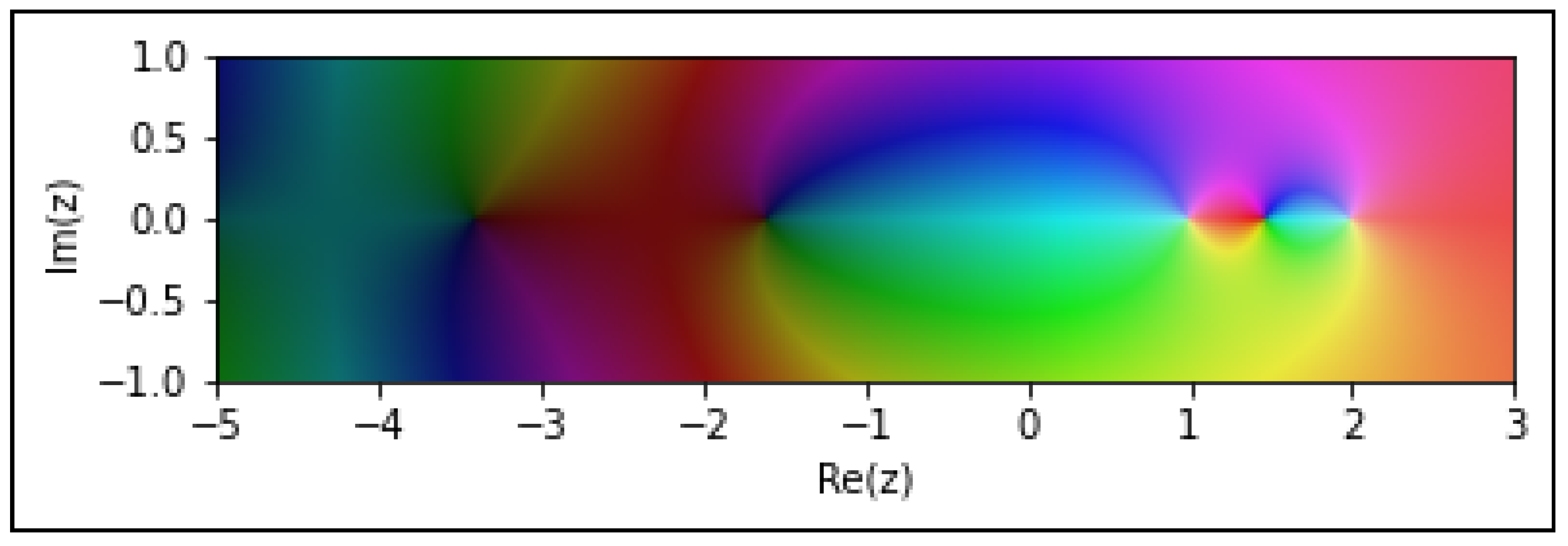
Figure 1.
F-Shah–Riemann zeta function for : . Two poles of the function are observed as and , whereas a positive real root can be observed at .
Figure 1.
F-Shah–Riemann zeta function for : . Two poles of the function are observed as and , whereas a positive real root can be observed at .
Figure 2.
F-Shah–Riemann zeta function for : . Three poles of the function are observed as and , whereas two positive real roots can be observed at and .
Figure 2.
F-Shah–Riemann zeta function for : . Three poles of the function are observed as and , whereas two positive real roots can be observed at and .
Figure 3.
F-Shah–Riemann zeta function for : . Four poles of the function are observed as and , whereas three positive real roots can be observed at and .
Figure 3.
F-Shah–Riemann zeta function for : . Four poles of the function are observed as and , whereas three positive real roots can be observed at and .
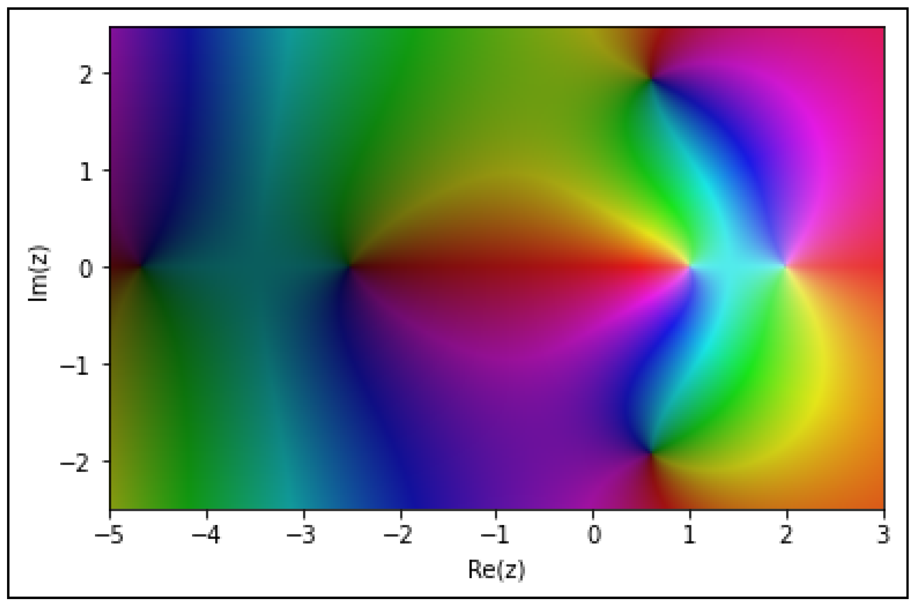
Figure 4.
C-Shah–Riemann zeta function for : . Two poles of the function are observed as and , whereas a pair of non-trivial complex roots can be observed at .
Figure 4.
C-Shah–Riemann zeta function for : . Two poles of the function are observed as and , whereas a pair of non-trivial complex roots can be observed at .
Figure 5.
C-Shah–Riemann zeta function for : . Three poles of the function are observed as and , whereas two pairs of non-trivial complex root can be observed at and .
Figure 5.
C-Shah–Riemann zeta function for : . Three poles of the function are observed as and , whereas two pairs of non-trivial complex root can be observed at and .
Figure 6.
C-Shah–Riemann zeta function for : . Four poles of the function are observed as and , whereas three pairs of non-trivial complex root can be observed at and .
Figure 6.
C-Shah–Riemann zeta function for : . Four poles of the function are observed as and , whereas three pairs of non-trivial complex root can be observed at and .
Table 1.
All of the positive (non-trivial) real zeros and some of the complex and negative (trivial) real zeros of F-Shah–Riemann zeta function for values of q = 2, q = 3 and up to 12 decimal places.
Table 1.
All of the positive (non-trivial) real zeros and some of the complex and negative (trivial) real zeros of F-Shah–Riemann zeta function for values of q = 2, q = 3 and up to 12 decimal places.
| Values of q | Complex Zeros | Non-Trivial Real Zeros | Trivial Real Zeros |
|---|
| q = 2 | 1.247595281027 + 14.148570425918i | 1.473414717168 | −1.606882014624 |
| 1.279113135722 + 21.012442575688i | - | −3.4037619981310 |
| q = 3 | 1.964049664859 + 14.165353520342i | 1.346727332380 | −1.346011820212 |
| 2.032696553488 + 21.001910485581i | 2.675764968478 | −2.878069065724 |
| 2.062342325067 + 25.053176875792i | - | −4.623564926958 |
| q = 4 | 2.653604262294 + 14.184700388061i | 1.271435903075 | −1.192688707675 |
| 2.763852133144 + 20.991263644295i | 2.551800083744 | −2.423972912304 |
| 2.811381226897 + 25.077915228667i | 3.796568180266 | −3.975616047809 |
| 2.852031019544 + 30.316385253077i | - | −5.736688777159 |
Table 2.
Some of the non-trivial and trivial complex and real zeros of for values of and up to 10 decimal places.
Table 2.
Some of the non-trivial and trivial complex and real zeros of for values of and up to 10 decimal places.
| Values of q | Trivial Complex Zeros | Non-Trivial Complex Zeros | Real Zeros |
|---|
| q = 2 | 2.0460386041 + 14.0894409779i | 0.6078048160 + 1.9350010902i | −2.514994862054 |
| 1.9443544646 + 21.0650038610i | 0.6078048160 − 1.9350010902i | −4.675064985091 |
| q = 3 | 3.2683247579 + 14.0859069231i | −0.6997539191 + 1.7534110356i | −3.180342471496 |
| 3.1531129164 + 21.0656065389i | 2.2160159281 + 2.0194666275i | −5.450484894914 |
| 3.1027440708 + 24.9358435149i | 2.2160159281 − 2.0194666275i | −7.577495596468 |
| q = 4 | 4.3760513879 + 14.0924715621i | −1.4515176098 + 1.2122471911i | −4.035452332431 |
| 4.2716503066 + 21.0555557135i | 0.8794024170 + 2.3478232248i | −6.316237379469 |
| 4.2263218286 + 24.9427024675i | 3.5554537875 + 1.9983004535i | −8.456827453077 |
| 4.1822154523 + 30.5605816189i | 3.5554537875 − 1.9983004535i | −10.54593349392 |
Table 3.
Some observed equivalent results for and .
Table 3.
Some observed equivalent results for and .
| Observed Equivalent Result for | Observed Equivalent Result for |
|---|
| | |
| | |
| | |
| | |
| | |
| | |
| Publisher’s Note: MDPI stays neutral with regard to jurisdictional claims in published maps and institutional affiliations. |
© 2022 by the authors. Licensee MDPI, Basel, Switzerland. This article is an open access article distributed under the terms and conditions of the Creative Commons Attribution (CC BY) license (https://creativecommons.org/licenses/by/4.0/).


 ,
, 


