Truncated Cauchy Power Weibull-G Class of Distributions: Bayesian and Non-Bayesian Inference Modelling for COVID-19 and Carbon Fiber Data

Abstract

The Truncated Cauchy Power Weibull-G class is presented as a new family of distributions. Unique models for this family are presented in this paper. The statistical aspects of the family are explored, including the expansion of the density function, moments, incomplete moments (IMOs), residual life and reversed residual life functions, and entropy. The maximum likelihood (ML) and Bayesian estimations are developed based on the Type-II censored sample. The properties of Bayes estimators of the parameters are studied under different loss functions (squared error loss function and LINEX loss function). To create Markov-chain Monte Carlo samples from the posterior density, the Metropolis–Hasting technique was used with posterior density. Using non-informative and informative priors, a full simulation technique was carried out. The maximum likelihood estimator was compared to the Bayesian estimators using Monte Carlo simulation. To compare the performances of the suggested estimators, a simulation study was carried out. Real-world data sets, such as strength measured in GPA for single carbon fibers and impregnated 1000-carbon fiber tows, maximum stress per cycle at 31,000 psi, and COVID-19 data were used to demonstrate the relevance and flexibility of the suggested method. The suggested models are then compared to comparable models such as the Marshall–Olkin alpha power exponential, the extended odd Weibull exponential, the Weibull–Rayleigh, the Weibull–Lomax, and the exponential Lomax distributions.

1. Introduction

In recent years, many authors have made a great effort to construct new families to extend existing well-known distributions and provide flexible classes to model data in various fields such as medical sciences and environmental, demographic, actuarial, and economic studies. Many generalized families were generated and extended to explain various phenomena in real data. Some examples of these families are beta-generated [1], gamma-generated [2], generalized Kumaraswamy [3], Marshall–Olkin alpha power-G [4], and odd Lomax-G [5], Type II half logistic-G in [6], transmuted odd Fréchet-G in [7], Type II exponentiated half logistic-G in [8], exponentiated M-G by [9], exponentiated truncated inverse Weibull-G in [10] among others.

A new wider family of distributions, called the odd Weibull-G (OW-G) family was created by [11]. The cumulative distribution function (CDF) and the corresponding probability density function (PDF) are

$$H_{WG}\left(x;\lambda ,\delta \right)={{\displaystyle \int }}_0^{\frac{G\left(x;\delta \right)}{1-G\left(x;\delta \right)}}\lambda t^{\lambda -1}{e}^{-t^{\lambda }dt}=1-e^{-{\left(\frac{G\left(x;\delta \right)}{\overline{G}\left(x;\delta \right)}\right)}^{\lambda },} \lambda >0, x,\delta \in R,$$

(1)

and

$$h_{WG}\left(x;\lambda ,\delta \right)=\lambda g\left(x;\delta \right)\frac{G{(x;\delta )}^{\lambda -1}}{\overline{G}{(x;\delta )}^{\lambda +1}}{e}^{-{\left(\frac{G\left(x;\delta \right)}{\overline{G}\left(x;\delta \right)}\right)}^{\lambda }},\lambda >0, x,\delta \in R,$$

(2)

where $\lambda$ is a shape parameter and $\delta$ is the vector of parameters of the parent distributions, $G\left(x;\delta \right)$ and $g\left(x;\delta \right)$ are the CDF and PDF of a baseline continuous distribution with $\delta$ as parameter vector, respectively.

Establishing new distributions is a hot topic in contemporary research. It offers more flexible distributions capable of modelling complicated data structures.

The Cauchy distribution is symmetric and has a very heavy tail, it is used in many applications such as econometrics, biological, spectroscopy, engineering studies, and theory of reliability. Many authors have shown the different aspects of generalization and extension of Cauchy distribution, for example, [12] provided a truncated Cauchy distribution, [13] introduced a Kumaraswamy–half-Cauchy distribution, and [14] presented the power-Cauchy negative-binomial distribution.

Recently, a new class called the truncated Cauchy power-G (TCP-G) class was proposed by [15]. The CDF and PDF of the TCP-G class, respectively, are proposed below:

$$F\left(x;\theta ,\delta \right)=\frac{4}{\pi }\arctan (H\left(x;\delta {)}^{\theta }\right),x,\delta \in R,\theta >0,$$

(3)

and

$$f\left(x;\theta ,\delta \right)=\frac{4\theta h\left(x;\delta \right){(H\left(x;\delta \right))}^{\theta -1}}{\pi \left[1+{(H\left(x;\delta \right))}^{2\theta }\right]},x,\delta \in R,\theta >0,$$

(4)

where $\theta$ is a shape parameter, $H\left(x;\delta \right)$ and $h\left(x;\delta \right)$ are the CDF and PDF of a baseline continuous distribution with $\delta$ as parameter vector, respectively.

The hazard rate function (hr) is

$$h\left(x;\theta ,\delta \right)=\frac{f\left(x;\theta ,\delta \right)}{\overline{F}\left(x;\theta ,\delta \right)}=\frac{f\left(x;\theta ,\delta \right)}{1-\mathrm{F}\left(x;\theta ,\delta \right)}=\frac{4\theta h\left(x;\delta \right){(H\left(x;\delta \right))}^{\theta -1}}{\pi \left[1+{(H\left(x;\delta \right))}^{2\theta }\right]\left[1-\frac{4}{\pi }\arctan (H\left(x;\delta {)}^{\theta }\right)\right]},$$

(5)

where $\overline{F}\left(x;\theta ,\delta \right)$ is the reliability function.

The main objective of this paper is:

• To present a new, wider, and flexible, family of distributions based on the W–G family and TCP family.
• The PDF of submodels of the suggested family can be decreasing, unimodal, right skewness, and symmetrically shaped. Additionally, the hazard function can be unimodal, U-shaped, J-shaped, increasing, decreasing, and constant.
• To investigate some of its statistical features, such as the quantile function, moments, incomplete moments and Rényi entropy.
• To discuss the statistical inference of the TCPW-G family by using the ML and Bayesian approaches.
• To conduct a simulation study to demonstrate the behavior of the parameters model.
• To provide better fits than some known models with favorable results for the TCPWE, TCPWR, and TCPWL models.

This family called the Truncated Cauchy Power Weibull-G (TCPW-G) family of distributions, which is created by inserting (1) into (3), with CDF and PDF, respectively, provided by

$$F\left(x;\theta ,\lambda ,\delta \right)=\frac{4}{\pi }\arctan {\left[1-e^{-{\left(\frac{G\left(x;\delta \right)}{\overline{G}\left(x;\delta \right)}\right)}^{\lambda }}\right]}^{\theta }, x,\delta \in R,\theta , \lambda >0,$$

(6)

and

$$f\left(x;\theta ,\lambda ,\delta \right)=\frac{4\theta \lambda }{\pi }g\left(x;\delta \right)\frac{G{(x;\delta )}^{\lambda -1}}{\overline{G}{(x;\delta )}^{\lambda +1}}{e}^{-{\left(\frac{G\left(x;\delta \right)}{\overline{G}\left(x;\delta \right)}\right)}^{\lambda }}{\left[1-e^{-{\left(\frac{G\left(x;\delta \right)}{\overline{G}\left(x;\delta \right)}\right)}^{\lambda }}\right]}^{\theta -1}{\left\{1+{\left[1-e^{-{\left(\frac{G\left(x;\delta \right)}{\overline{G}\left(x;\delta \right)}\right)}^{\lambda }}\right]}^{2\theta }\right\}}^{-1} , x,\delta \in R,\theta , \lambda >0.$$

(7)

We will denote a random variable $X$ with PDF (7) by $X~TCPW\left(\theta ,\lambda ,\delta \right).$ The reliability and hazard rate functions for the $TCPW-G$ family are, respectively, given by $\overline{F}\left(x;\theta ,\lambda ,\delta \right)=1-\mathrm{F}\left(x;\theta ,\lambda ,\delta \right),$ and $\tau \left(x;\theta ,\lambda ,\delta \right)=\frac{f\left(x;\theta ,\lambda ,\delta \right)}{\overline{F}\left(x;\theta ,\lambda ,\delta \right)}$.

The outline for this paper is as follows. Section 2 includes a valuable extension of the TCPW density as well as three sub-models. Section 3 investigates the basic statistical properties of the TCPW-G family. In Section 4, the family’s unknown parameters are estimated using Bayesian and non-Bayesian approaches. Section investigates Type-II censoring techniques. In Section 6, Monte Carlo simulation is used to compare the MLE and Bayesian parameters of the TCPWE. In Section 7, we present two real-world examples to show the versatility of the TCPW-G family.

2. Expansion and Sub-Models

In this section, we look at various helpful expansion functions that are based on the generalized binomial series. If $\left|\hspace{0.17em}z\hspace{0.17em}\right|<1$ and $b>0$ are real non-integers, with the accompanying power series:

$${(1+z)}^{-b}={{\displaystyle \sum }}_{i=0}^{\infty }{(-1)}^i\frac{\mathsf{\Gamma }\left(b+i\right)}{\mathsf{\Gamma }\left(i+1\right)\mathsf{\Gamma }\left(b\right)}{z}^i,$$

(8)

and

$${(1-z)}^{b-1}={{\displaystyle \sum }}_{j=0}^{\infty }{(-1)}^j\frac{\mathsf{\Gamma }\left(b\right)}{\mathsf{\Gamma }\left(j+1\right)\mathsf{\Gamma }\left(b-j\right)}{z}^j,$$

(9)

Applying (8) to the last term in (7), it becomes

$$f_{TCPW}\left(x;\theta ,\lambda ,\delta \right)=\frac{4\theta \lambda }{\pi }g\left(x;\delta \right)\frac{G{(x;\delta )}^{\lambda -1}}{\overline{G}{(x;\delta )}^{\lambda +1}}{e}^{-{\left(\frac{G\left(x;\delta \right)}{\overline{G}\left(x;\delta \right)}\right)}^{\lambda }}{{\displaystyle \sum }}_{i=0}^{\infty }{(-1)}^i{\left[1-e^{-{\left(\frac{G\left(x;\delta \right)}{\overline{G}\left(x;\delta \right)}\right)}^{\lambda }}\right]}^{\theta \left(2i+1\right)-1}.$$

(10)

In addition, using (9) in (10), the TCPW-G density can be written as

$$f_{TCPW}\left(x;\theta ,\lambda ,\delta \right)=\frac{4\theta \lambda }{\pi }g\left(x;\delta \right)\frac{G{(x;\delta )}^{\lambda -1}}{\overline{G}{(x;\delta )}^{\lambda +1}}{{\displaystyle \sum }}_{i,j=0}^{\infty }{(-1)}^{i+j}\frac{\mathsf{\Gamma }\left(\theta \left(2i+1\right)\right)}{\mathsf{\Gamma }\left(j+1\right)\mathsf{\Gamma }\left(\theta \left(2i+1\right)-\mathrm{j}\right)}{e}^{-\left(j+1\right){\left(\frac{G\left(x;\delta \right)}{\overline{G}\left(x;\delta \right)}\right)}^{\lambda }},$$

(11)

and by expanding $e^{-\left(j+1\right){\left(\frac{G\left(x;\delta \right)}{\overline{G}\left(x;\delta \right)}\right)}^{\lambda }}$ in a power series of the exponential function, we can write

$$e^{-\left(j+1\right){\left(\frac{G\left(x;\delta \right)}{\overline{G}\left(x;\delta \right)}\right)}^{\lambda }}={\displaystyle \sum }_{k=0}^{\infty }\frac{{(-1)}^k{(j+1)}^k}{k!}\frac{G{(x;\delta )}^{\lambda k}}{\overline{G}{(x;\delta )}^{\lambda k}}.$$

If we insert the above term in (11), we have

$$f{}_{TCPW}\left(x;\theta ,\lambda ,\delta \right)=\frac{4\theta \lambda }{\pi }g\left(x;\delta \right){{\displaystyle \sum }}_{i,j=0}^{\infty }{(-1)}^{i+j}\frac{\mathsf{\Gamma }\left(\theta \left(2i+1\right)\right)}{\mathsf{\Gamma }\left(j+1\right)\mathsf{\Gamma }\left(\theta \left(2i+1\right)-\mathrm{j}\right)}{{\displaystyle \sum }}_{k=0}^{\infty }\frac{{(-1)}^k}{k!}\frac{G{(x;\delta )}^{\lambda \left(k+1\right)-1}}{\overline{G}{(x;\delta )}^{\lambda \left(k+1\right)+1}},$$

(12)

and if the power series ${(1-z)}^{-b}={{\displaystyle \sum }}_{d=0}^{\infty }\frac{\mathsf{\Gamma }\left(b+d\right)}{\mathsf{\Gamma }\left(d+1\right)\mathsf{\Gamma }\left(b\right)}{z}^d$ is applied into (12), the$TCPW-G$ density may be written as an endless linear combination of exponentiated-G (Exp-G) PDFs

$$f{}_{TCPW}\left(x;\theta ,\lambda ,\delta \right)={{\displaystyle \sum }}_{k,d=0}^{\infty }{\varphi }_{k,d}{\pi }_{\left(\lambda \left(k+1\right)+d\right)}\left(x\right),$$

(13)

where ${\pi }_{\mathsf{\alpha }}\left(x\right)=\mathsf{\alpha }g\left(x\right)G^{\mathsf{\alpha }-1}\left(x\right)$ is the Exp-G PDF with power parameter α and

$${\varphi }_{k,d}={\displaystyle \sum }_{i,j=0}^{\infty }\frac{4\theta \lambda {(-1)}^{i+j+k}{(j+1)}^k}{\pi k!\left(\lambda \left(k+1\right)+d\right)}\frac{\mathsf{\Gamma }\left(\theta \left(2i+1\right)\right)}{\mathsf{\Gamma }\left(j+1\right)\mathsf{\Gamma }\left(\theta \left(2i+1\right)-\mathrm{j}\right)}\frac{\mathsf{\Gamma }\left(\lambda \left(k+1\right)+2\right)}{\mathsf{\Gamma }\left(d+1\right)\mathsf{\Gamma }\left(\lambda \left(k+1\right)-\mathrm{d}+2\right)}.$$

Thus, Equation (13) shows that the TCPW-G density is a mixture of the Exp-G densities with the parameter $\left(\lambda \left(k+1\right)+d\right).$ Consequently, we can derive the statistical properties of the TCPW-G family from those of Exp-G. Similarly, the CDF TCPW families can also be represented as a linear combination as follows:

$F{}_{TCPW}\left(x;\theta ,\lambda ,\delta \right)={\displaystyle \sum }_{k,d=0}^{\infty }{\varphi }_{k,d}{\Pi }_{\left(\lambda \left(k+1\right)+d\right)}\left(x\right),$ where ${\Pi }_{\left(\lambda \left(k+1\right)+d\right)}\left(x\right)$ is the Exp-G CDF with power parameter $\left(\lambda \left(k+1\right)+d\right)$.

2.1. Some Special Models of the TCPW-G Family

Among the many different distributions arising from the TCPW-G family of distributions, we now present three special cases using classic distributions as baselines.

2.1.1. Truncated Cauchy Power Weibull Lomax (TCPWL) Distribution

The TCPW family has a Lomax distribution as the baseline distribution, i.e., with $G\left(x\right)=1-{(1+\frac{x}{\beta })}^{-\alpha }$ $\mathrm{and}g\left(x\right)=\frac{\alpha }{\beta }{(1+\frac{x}{\beta })}^{-\alpha -1}$ and the CDF and PDF of TCPWL distribution of

$$F\left(x;\theta ,\lambda ,\alpha ,\beta \right)=\frac{4}{\pi }\arctan {\left[1-e^{-{\left({(1+\frac{x}{\beta })}^{\alpha }-1\right)}^{\lambda }}\right]}^{\theta },x, \theta ,\lambda ,\alpha ,\beta >0,$$

(14)

and

$$\begin{gathered} f\left(x;\theta ,\lambda ,\alpha ,\beta \right)=\frac{4\theta \lambda \alpha }{\pi \beta }{(1+\frac{x}{\beta })}^{-\alpha -1}\frac{{(1-{(1+\frac{x}{\beta })}^{-\alpha })}^{\lambda -1}}{{({(1+\frac{x}{\beta })}^{-\alpha })}^{\lambda +1}}{e}^{-{\left({(1+\frac{x}{\beta })}^{\alpha }-1\right)}^{\lambda }}{\left[1-e^{-{\left({(1+\frac{x}{\beta })}^{\alpha }-1\right)}^{\lambda }}\right]}^{\theta -1} \\ {\left\{1+{\left[1-e^{-{\left({(1+\frac{x}{\beta })}^{\alpha }-1\right)}^{\lambda }}\right]}^{2\theta }\right\}}^{-1} ,x, \theta ,\lambda ,\alpha ,\beta >0, \end{gathered}$$

(15)

where $\alpha \mathrm{and}\beta$ are two shape parameters.

2.1.2. Truncated Cauchy Power Weibull Exponential (TCPWE) Distribution

The TCPW family has an exponential distribution as the baseline distribution, i.e., with $G\left(x\right)=1-e^{-\mu x} and g\left(x\right)=\mu e^{-\mu x}.$ The CDF and the PDF of the TCPWE model are provided through

$$F\left(x;\theta ,\lambda ,\mu \right)=\frac{4}{\pi }\arctan {\left[1-e^{-{\left(e^{\mu x}-1\right)}^{\lambda }}\right]}^{\theta },x, \theta ,\lambda ,\mu >0,$$

(16)

and

$$f\left(x;\theta ,\lambda ,\mu \right)=\frac{4\theta \lambda \mu }{\pi }{e}^{-\mu x}\frac{{(1-e^{-\mu x})}^{\lambda -1}}{{(e^{-\mu x})}^{\lambda +1}}{e}^{-{\left(e^{\mu x}-1\right)}^{\lambda }}{\left[1-e^{-{\left(e^{\mu x}-1\right)}^{\lambda }}\right]}^{\theta -1}{\left\{1+{\left[1-e^{-{\left(e^{\mu x}-1\right)}^{\lambda }}\right]}^{2\theta }\right\}}^{-1} ,x, \theta ,\lambda ,\mu >0,$$

(17)

where $\mu$ is a scale parameter.

2.1.3. Truncated Cauchy Power Weibull Rayleigh (TCPWR) Distribution

The TCPW family has a Rayleigh distribution as the baseline distribution; i.e., it has $\left(x\right)=1-e^{-\frac{\rho }{2}{x}^2}$ $\mathrm{and}g\left(x\right)=\rho x{e}^{-\frac{\rho }{2}{x}^2}$. The CDF and the PDF of the TCPWR model are provided through

$$F\left(x;\theta ,\lambda ,\rho \right)=\frac{4}{\pi }\arctan {\left[1-e^{-{\left(e^{\frac{\rho }{2}{x}^2}-1\right)}^{\lambda }}\right]}^{\theta },x, \theta ,\lambda ,\rho >0,$$

(18)

and

$$f\left(x;\theta ,\lambda ,\rho \right)=\frac{4\theta \lambda \rho }{\pi }x{e}^{-\frac{\rho }{2}{x}^2}\frac{{(1-e^{-\frac{\rho }{2}{x}^2})}^{\lambda -1}}{{(e^{-\frac{\rho }{2}{x}^2})}^{\lambda +1}}{e}^{-{\left(e^{\frac{\rho }{2}{x}^2}-1\right)}^{\lambda }}\frac{{\left[1-e^{-{\left(e^{\frac{\rho }{2}{x}^2}-1\right)}^{\lambda }}\right]}^{\theta -1}}{1+{\left[1-e^{-{\left(e^{\frac{\rho }{2}{x}^2}-1\right)}^{\lambda }}\right]}^{2\theta }},x, \theta ,\lambda ,\rho >0,$$

(19)

where $\rho$ is a scale parameter.

From the Figure 1, Figure 2 and Figure 3 we can note the PDF of TCPWL, TCPWE, and TCPWR can be decreasing, unimodal, right skewness and symmetric shaped. Additionally, the hazard function can be unimodal, U-shaped, J-shaped, increasing, decreasing, and constant.

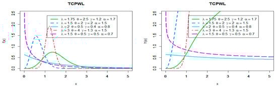
Figure 1. Plots of PDF and the hazard function of TCPWL distribution.

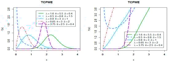
Figure 2. Plots of PDF and the hazard function of TCPWE distribution.

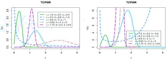
Figure 3. Plots of PDF and the hazard function of TCPWR distribution.

3. Statistical Features

In this section, we will discuss some statistical features of the TCPW class of distributions.

3.1. Quantile Function

By inverting (6), we obtain the TCPW quantile function (QF), say, $x=Q\left(u\right)$, as follows:

$$F^{-1}\left(u\right)=Q_G\left(u\right)=G^{-1}\left[\frac{-\frac{1}{\lambda }\mathit{log}\left[1-{\left[\mathit{tan}(\frac{u\pi }{4})\right]}^{\frac{1}{\theta }}\right]}{1+\left\{-\frac{1}{\lambda }\mathit{log}\left[1-{\left[\mathit{tan}(\frac{u\pi }{4})\right]}^{\frac{1}{\theta }}\right]\right\}}\right],$$

(20)

where $Q_{G\left(u\right)}$ denotes the function corresponding to $G\left(x\right)$. $Q\left(u\right)$ is characterized by the non-linear equation $F\left(Q\left(u\right)\right)=Q\left(F\left(u\right)\right)=u$, $u\in \left(0,1\right)$, where $Q(.)$ represents the quantile function for any parent distributions $G\left(x;\delta \right)$.

Figure 4 and Figure 5 show the skewness and kurtosis plots for TCPWE distribution with different values of parameters when $\rho =2$ and $\rho =5$.

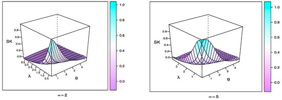
Figure 4. Skewness plot for TCPWE distribution with different values of parameters when $\rho =2$ and $\rho =5$.

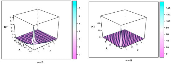
Figure 5. Kurtosis plot for TCPWE distribution with different values of parameters when $\rho =2$ and $\rho =5$.

3.2. Moments

This sub-section derives the ordinary-moment and moment-generating functions of the $TCPW$ family. The skewness, kurtosis, and expected lifetime of a device can be obtained from the moments.

3.2.1. Ordinary Moments

Let $J_{\left(\lambda \left(k+1\right)+d\right))}$ be a random variable to have the Exp-G PDF with the power parameter $\left(\lambda \left(k+1\right)+d\right).$ The$r^{th}\mathrm{moment}$ of the TCPW class of distributions can be determined from (13) as

$${\stackrel{`}{\mu }}_r=E\left(X^r\right)={{\displaystyle \sum }}_{k,d=0}^{\infty }{\varphi }_{k,d}E\left(J_{\left(\lambda \left(k+1\right)+d\right)}^r\right).$$

(21)

For $\beta >0,\mathrm{The} r^{th}\mathrm{moment}\mathrm{of}$ the Exp-G distribution with power parameter $\left(\lambda \left(k+1\right)+d\right)$ can be proposed by

$$E\left(J_{\beta }^r\right)=\beta {{\displaystyle \int }}_{-\infty }^{\infty }{x}^{r}g\left(x; \delta \right)G{(x; \delta )}^{\beta -1},\mathrm{or}E\left(J_{\beta }^r\right)=\beta {{\displaystyle \int }}_0^1{u}^{\beta -1}{Q}_G{(u; \delta )}^{r}du,$$

where $Q_G\left(u; \delta \right)=G^{-1}\left(u; \delta \right)$.

We have now shown two formulas for the moment generating function. From Equation (13), we may obtain the first of the following formulas:

$$M_X\left(t\right)=E\left(e^{tX}\right)={{\displaystyle \sum }}_{k,d=0}^{\infty }{\varphi }_{k,d}{M}_{\left(\lambda \left(k+1\right)+d\right)}\left(t\right),$$

(22)

where $M_{\left(\lambda \left(k+1\right)+d\right)}\left(t\right)$ is the moment generating function of $J_{\left(\lambda \left(k+1\right)+d\right)}$. Consequently, we can easily calculate $M_X\left(t\right)$ from the Exp-G generating function. The second formula for the moment generating function of the TCPW class of distributions is based on the baseline quantile function as

$$M_X\left(t\right)=E\left(e^{tX}\right)={\displaystyle \sum }_{k,d=0}^{\infty }{\varphi }_{k,d}{\nu }_{\left(\mathrm{t},\lambda \left(k+1\right)+d\right)},$$

where

$${\nu }_{\left(\mathrm{t},s\right)}=k{{\displaystyle \int }}_0^1{u}^{s-1}{e}^{t{Q}_G\left(u; \delta \right)}du.$$

3.2.2. Conditional Moments

Incomplete moments are commonly used to describe the Bonferroni and Lorenz curves, which are both essential in many domains such as reliability theory, finance, economics, and demography. The incomplete moments $s^{th}$ of X denoted by ${\kappa }_s\left(t\right)$ for any real $s>0$ is defined from (13) as

$${\kappa }_s\left(t\right)={{\displaystyle \int }}_{-\infty }^t{x}^{s}f\left(x\right)dx={{\displaystyle \sum }}_{k,d=0}^{\infty }{\varphi }_{k,d}{{\displaystyle \int }}_{-\infty }^t{x}^s{\kappa }_{s,\left(\lambda \left(k+1\right)+d\right)}\left(t\right)dx,$$

(23)

where ${\kappa }_{s,\omega }\left(t\right)={{\displaystyle \int }}_0^{G\left(t\right)}{u}^{\omega -1}{Q}_G{(u)}^{s}du$ and ${\kappa }_{s,\omega }\left(t\right)$ can be calculated numerically.

The mean deviations provide essential information on population characteristics and have also been used in income fields and economics. If $X$ has the TCPW family of distribution, the mean deviations about the mean $E\left(X\right)$ and the mean deviations about the median are defined by

$${\delta }_{\mu }\left(x\right)=E\hspace{0.17em}\left|\hspace{0.17em}X-E\left(X\right)\hspace{0.17em}\right|=2E\left(X\right)F\left(E\left(X\right)\right)-2{\kappa }_{1}E\left(X\right)),$$

(24)

and

$${\delta }_M\left(x\right)=E\hspace{0.17em}\left|\hspace{0.17em}X-\mathrm{median}\left(X\right)\hspace{0.17em}\right|={\stackrel{`}{\mu }}_1-2{\kappa }_1\left(\mathrm{median}\left(X\right)\right),$$

(25)

respectively, where ${\kappa }_1\left(t\right)$ is the first complete moment given by (23) with $s=1$.

The Lorenz and Bonferroni curves of the TCPW class of distributions for a given probability $\pi$ can be written as $L\left(\pi \right)=\frac{1}{{\stackrel{`}{\mu }}_1}{\kappa }_1\left(q\right)$ and $B\left(\pi \right)=\frac{1}{\pi {\stackrel{`}{\mu }}_1}{\kappa }_1\left(q\right)$, respectively, where ${\stackrel{`}{\mu }}_1=E\left(X\right)$ and $q=Q\left(\pi \right)$ is the QF of $X$ at $\pi$.

The $r^{th}$ moment of the residual life is provided by

$$\begin{gathered} {\mu }_r\left(t\right)=E(\left(X-t{)}^r\hspace{0.17em}|\hspace{0.17em}X>t\right)=\frac{1}{\overline{F}\left(t\right)}{{\displaystyle \int }}_t^{\infty }{(x-t)}^{r}f\left(x\right)dx,r\ge 1 \\ =\frac{1}{\overline{F}\left(t\right)}{\sum }_{k,d=0}^{\infty }{\varphi }_{k,d}^{*}{\int }_t^{\infty }{x}^r{\pi }_{\left(\lambda \left(k+1\right)+d\right)}\left(x\right)dx. \end{gathered}$$

(26)

where ${\varphi }_{k,d}^{*}={\varphi }_{k,d}{\sum }_{m=0}^r\left(\begin{array}{c}r\\ m\end{array}\right){(-t)}^{r-m}$.

The $r^{th}$ moment of the reversed residual life is provided by

$$\begin{gathered} m_r\left(t\right)=E({(t-X)}^r\hspace{0.17em}|\hspace{0.17em}X\le t)=\frac{1}{F\left(t\right)}{{\displaystyle \int }}_0^t{(t-x)}^{r}f\left(x\right)dx,r\ge 1 \\ =\frac{1}{F\left(t\right)}{\displaystyle \sum }_{k,d=0}^{\infty }{\varphi }_{k,d}^{*}{{\displaystyle \int }}_0^t{x}^r{\pi }_{\left(\lambda \left(k+1\right)+d\right)}\left(x\right)dx \end{gathered}$$

(27)

3.3. Rényi Entropy

The Rényi entropy is provided by ($\rho >0,\rho \ne 1)$

$$I_R\left(\rho \right)=\frac{1}{1-\rho }\log \left[{{\displaystyle \int }}_{-\infty }^{\infty }f{}^{\rho }\left(x\right)dx\right].$$

(28)

Utilizing (7), the same procedure as the beneficial expansion (13) and some simplifications, we acquire

$$f^{\rho }\left(x\right)={{\displaystyle \sum }}_{k,d=0}^{\infty }{\varpi }_{k,d}g{(x)}^{\rho }G{(x)}^{\lambda \left(k+\rho \right)+d-\rho },$$

(29)

where ${\varpi }_{k,d}={{\displaystyle \sum }}_{i,j=0}^{\infty }\frac{4\theta {\lambda }^{\rho }}{\pi }\frac{{\left(-1\right)}^{i+j+k}{\left(j+\rho \right)}^k\mathsf{\Gamma }\left(\theta \left(2i+\rho \right)-\rho +1\right)\mathsf{\Gamma }\left(\lambda \left(\rho +k\right)+2\right)}{k!d!\mathsf{\Gamma }\left(j+1\right)\mathsf{\Gamma }\left(\theta \left(2i+\rho \right)-\rho -j+1\right)\mathsf{\Gamma }\left(d+1\right)\mathsf{\Gamma }\left(\lambda \left(\rho +k\right)-d+2\right)}$.

Thus, Rényi entropy of $TCPW$ family is provided by

$$I_R\left(\rho \right)=\frac{1}{1-\rho }\log \left\{{{\displaystyle \sum }}_{k,d=0}^{\infty }{\varpi }_{k,d}{{\displaystyle \int }}_{-\infty }^{\infty }g{(x)}^{\rho }G{(x)}^{\lambda \left(k+\rho \right)+d-\rho }dx\right\}.$$

(30)

4. Bayesian and Non-Bayesian Estimation Methods

4.1. Maximum Likelihood Estimation

Let $x_1,\dots ,x_n$ be a random sample of size $n$ from the TCPW distribution. The log-likelihood function for $\Phi =$(θ$,\lambda ,\delta {)}^T$ is the $q\times 1$ vector of parameters, given by

$$\begin{gathered} L_n\left(\Phi \right)=n log(\frac{4\theta }{\pi })+n log(\lambda )+{\displaystyle \sum }_{i=1}^{n}log g\left(x_i;\delta \right)+\left(\lambda -1\right){\displaystyle \sum }_{i=1}^n log G\left(x_i;\delta \right)-\left(\lambda +1\right){\displaystyle \sum }_{i=1}^{n}log(\overline{G}\left(x_i;\delta \right))-{\displaystyle \sum }_{i=1}^n{z}_i+\left(\theta -1\right){\displaystyle \sum }_{i=1}^{n}log\left[1-e^{-{\left(z_i\right)}^{\lambda }}\right]- \\ {{\displaystyle \sum }}_{i=1}^{n}log\left\{1+{\left[1-e^{-{\left(z_i\right)}^{\lambda }}\right]}^{2\theta }\right\}, \end{gathered}$$

(31)

where $z_i=\frac{G\left(x_i;\delta \right)}{\overline{G}\left(x_i;\delta \right)}.$ The components of the score function $U\left(\Phi \right)=\left(U_{\theta },U_{\lambda },U_{\delta }\right)$ are

$$\begin{gathered} U_{\theta }=\frac{\partial L_n}{\partial \theta }=\frac{n}{\theta }+{{\displaystyle \sum }}_{i=1}^{n}log\left[1-e^{-{\left(z_i\right)}^{\lambda }}\right]-{{\displaystyle \sum }}_{i=1}^n\frac{2{\left[1-e^{-{\left(z_i\right)}^{\lambda }}\right]}^{2\theta }log\left[1-e^{-{\left(z_i\right)}^{\lambda }}\right]}{1+{\left[1-e^{-{\left(z_i\right)}^{\lambda }}\right]}^{2\theta }},. \\ {U}_{\lambda }=\frac{\partial L_n}{\partial \lambda }=\frac{n}{\lambda }+{{\displaystyle \sum }}_{i=1}^{n}log G\left(x_i;\delta \right)-{{\displaystyle \sum }}_{i=1}^{n}log(\overline{G}\left(x_i;\delta \right))+\left(\theta -1\right){{\displaystyle \sum }}_{i=1}^n\frac{e^{-{\left(z_i\right)}^{\lambda }}{\left(z_i\right)}^{\lambda }log\left(z_i\right)}{1-e^{-{\left(z_i\right)}^{\lambda }}}-{{\displaystyle \sum }}_{i=1}^n\frac{2\theta {\left[1-e^{-{\left(z_i\right)}^{\lambda }}\right]}^{2\theta -1}{e}^{-{\left(z_i\right)}^{\lambda }}{\left(z_i\right)}^{\lambda }log\left(z_i\right)}{1+{\left[1-e^{-{\left(z_i\right)}^{\lambda }}\right]}^{2\theta }}, \end{gathered}$$

and

$$\begin{gathered} U_{\delta }=\frac{\partial L_n}{\partial \delta }={\displaystyle \sum }_{i=1}^n\frac{g^{\prime }\left(x_i;\delta \right)}{g\left(x_i;\delta \right)}+\left(\lambda -1\right){\displaystyle \sum }_{i=1}^n\frac{G^{\prime }\left(x_i;\delta \right)}{G\left(x_i;\delta \right)}-\left(\lambda +1\right){\displaystyle \sum }_{i=1}^n\frac{{\overline{G}}^{\text{’}}\left(x_i;\delta \right)}{\overline{G}\left(x_i;\delta \right)}-{\displaystyle \sum }_{i=1}^n\left(\frac{\partial z_i}{\partial {\delta }_k}\right)+ \\ \left(\theta -1\right){{\displaystyle \sum }}_{i=1}^n\frac{\lambda {\left(z_i\right)}^{\lambda -1}{e}^{-{\left(z_i\right)}^{\lambda }}\left(\frac{\partial z_i}{\partial \delta }\right)}{1-e^{-{\left(z_i\right)}^{\lambda }}}-{{\displaystyle \sum }}_{i=1}^n\frac{2\theta \lambda {\left(z_i\right)}^{\lambda -1}{e}^{-{\left(z_i\right)}^{\lambda }}{\left[1-e^{-{\left(z_i\right)}^{\lambda }}\right]}^{2\theta -1}\left(\frac{\partial z_i}{\partial \delta }\right)}{1+{\left[1-e^{-{\left(z_i\right)}^{\lambda }}\right]}^{2\theta }}, \end{gathered}$$

where $g^{\prime }\left(x_i;\delta \right)=\frac{\partial g\left(x_i;\delta \right)}{\partial \delta },G^{\prime }\left(x_i;\delta \right)=\frac{\partial G\left(x_i;\delta \right)}{\partial \delta },$ and ${\overline{G}}^{\text{’}}\left(x_i;\delta \right)=\frac{\partial \overline{G}\left(x_i;\delta \right)}{\partial \delta }$.

The maximum likelihood estimation (MLEs) can be obtained numerically by solving the non-linear equations simultaneously: $\frac{\partial L_n}{\partial \theta }=\frac{\partial L_n}{\partial \lambda }=\frac{\partial L_n}{\partial \delta }=0.$ Iterative methods such as the Newton–Raphson type algorithms can be used.

4.2. Bayesian Estimation

The Bayesian estimation method depends on an informative prior; let $x_1,x_2,\dots ,x_n$ be a random-sample, distributed TCPW-G family with unknown parameters for the TCPWE or TCPWR distribution. To calculate the Bayesian estimation, we choose a prior distribution that is the independent from the gamma distributions. The independent joint prior density function of $\lambda , \mathsf{\theta }$ and $\delta$ is supplied by

$$\pi \left(\lambda ,\theta ,\delta \right)=\frac{b_1^{a_1}}{\gamma \left(a_1\right)}\frac{b_2^{a_2}}{\gamma \left(a_2\right)}\frac{b_3^{a_3}}{\gamma \left(a_3\right)}{\lambda }^{a_1-1}{\theta }^{a_2-1}{\delta }^{a_3-1}{e}^{-\left(b_1\lambda +b_2\theta +b_3\delta \right)}.$$

(32)

The joint posterior density function of $\lambda , \mathsf{\theta }$, and $\delta$ is obtained from likelihood and joint prior functions as follows:

$${\pi }^{*}\left(\lambda ,\theta ,\delta |\underset{\_}{x}\right)=\frac{\ell \left(\underset{\_}{x}|\lambda ,\theta ,\delta \right).\pi \left(\lambda ,\theta ,\delta \right)}{{{\displaystyle \int }}_{\delta }{{\displaystyle \int }}_{\mathsf{\theta }}{{\displaystyle \int }}_{\lambda }\ell \left(\underset{\_}{x}|\lambda ,\theta ,\delta \right).\pi \left(\lambda ,\theta ,\delta \right)d\lambda d\mathsf{\theta }d\delta },$$

(33)

where $\underset{\_}{x}=x_1, x_2,\dots ,x_n$. Then, the joint posterior of TCPW-G class can be expressed as

$$\begin{gathered} {\pi }^{*}\left(\lambda ,\theta ,\delta |\underset{\_}{x}\right)\propto {{\displaystyle \prod }}_{i=1}^{n}g\left(x_i;\delta \right)\frac{G{(x_i;\delta )}^{\lambda -1}}{\overline{G}{(x_i;\delta )}^{\lambda +1}}{\left[1-e^{-{\left(\frac{G\left(x_i;\delta \right)}{\overline{G}\left(x_i;\delta \right)}\right)}^{\lambda }}\right]}^{\theta -1}{\lambda }^{n+a_1-1}{\theta }^{n+a_2-1}{\delta }^{n+a_3-1}{e}^{-{\displaystyle \sum }_{i=1}^n{\left(\frac{G\left(x_i;\delta \right)}{\overline{G}\left(x_i;\delta \right)}\right)}^{\lambda }} \\ {\left\{1+{\left[1-e^{-{\left(\frac{G\left(x_i;\delta \right)}{\overline{G}\left(x_i;\delta \right)}\right)}^{\lambda }}\right]}^{2\theta }\right\}}^{-1}{e}^{-\left(b_1\lambda +b_2\theta +b_3\delta \right)}. \end{gathered}$$

(34)

Under the symmetric and asymmetric loss functions, the loss function is important in the Bayesian estimation method. Square error (SE) is a well-known symmetric loss function, which can also be called the posterior mean, and it is defined as

$${\widehat{p}}_{SE}\left(\lambda ,\theta ,\delta \right)=E_{\lambda ,\theta ,\delta |\underset{\_}{x}}\left(p\left(\lambda ,\theta ,\delta \right)\right)={{\displaystyle \iiint }}_0^{\infty }\left(p\left(\lambda ,\theta ,\delta \right)\right){\pi }^{*}\left(\lambda ,\theta ,\delta |\underset{\_}{x}\right)d\lambda \mathrm{d}\theta \mathrm{d}\delta .$$

(35)

LINEX loss is well-known as an asymmetric loss function, and it can be defined as

$${\widehat{\mathsf{\Phi }}}_{Linex}=\frac{-1}{u}log\left(E(e^{-u\mathsf{\Phi }}|X)\right)$$

(36)

See [16,17] for further details on Bayesian estimation. We obviously cannot obtain explicit formulations for the expectation of the marginal posterior distribution for each and every parameter. As a result, the Markov Chain Monte Carlo (MCMC) approach is used to approximate the value of integrals. Gibbs sampling and, more broadly, Metropolis within Gibbs samplers are key subclasses of MCMC approaches. The Gibbs approach reduces the combined posterior distribution into a whole conditional distribution for each parameter. From PBLJ, the posterior conditional PDF of $\lambda$ given $\theta ,\delta$ can be obtained as

$${\pi }^{*}\left(\lambda |\theta ,\delta ,\underset{\_}{x}\right)\propto {{\displaystyle \prod }}_{i=1}^n\frac{G{(x_i;\delta )}^{\lambda -1}}{\overline{G}{(x_i;\delta )}^{\lambda +1}}{\left[1-e^{-{\left(\frac{G\left(x_i;\delta \right)}{\overline{G}\left(x_i;\delta \right)}\right)}^{\lambda }}\right]}^{\theta -1}{\lambda }^{n+a_1-1}{e}^{-\left(b_1\lambda \right)}{e}^{-{\displaystyle \sum }_{i=1}^n{\left(\frac{G\left(x_i;\delta \right)}{\overline{G}\left(x_i;\delta \right)}\right)}^{\lambda }}{\left\{1+{\left[1-e^{-{\left(\frac{G\left(x_i;\delta \right)}{\overline{G}\left(x_i;\delta \right)}\right)}^{\lambda }}\right]}^{2\theta }\right\}}^{-1}.$$

In a similar way, the posterior conditional PDF of $\theta$ given $\lambda ,\delta$ are provided by

$${\pi }^{*}\left(\theta |\lambda ,\delta ,\underset{\_}{x}\right)\propto {\theta }^{n+a_2-1}{e}^{-\left(b_2\theta \right)}{{\displaystyle \prod }}_{i=1}^n{\left[1-e^{-{\left(\frac{G\left(x_i;\delta \right)}{\overline{G}\left(x_i;\delta \right)}\right)}^{\lambda }}\right]}^{\theta -1}{\left\{1+{\left[1-e^{-{\left(\frac{G\left(x_i;\delta \right)}{\overline{G}\left(x_i;\delta \right)}\right)}^{\lambda }}\right]}^{2\theta }\right\}}^{-1}.$$

In a similar way, the posterior conditional PDF of $\delta$ given $\lambda ,\theta$. are provided by

$$\begin{gathered} {\pi }^{*}\left(\delta |\theta ,\lambda ,\underset{\_}{x}\right)\propto e^{-\left(b_3\delta \right)}{\delta }^{n+a_3-1}{{\displaystyle \prod }}_{i=1}^{n}g\left(x_i;\delta \right)\frac{G{(x_i;\delta )}^{\lambda -1}}{\overline{G}{(x_i;\delta )}^{\lambda +1}}{\left[1-e^{-{\left(\frac{G\left(x_i;\delta \right)}{\overline{G}\left(x_i;\delta \right)}\right)}^{\lambda }}\right]}^{\theta -1}{e}^{-{\displaystyle \sum }_{i=1}^n{\left(\frac{G\left(x_i;\delta \right)}{\overline{G}\left(x_i;\delta \right)}\right)}^{\lambda }} \\ {\left\{1+{\left[1-e^{-{\left(\frac{G\left(x_i;\delta \right)}{\overline{G}\left(x_i;\delta \right)}\right)}^{\lambda }}\right]}^{2\theta }\right\}}^{-1}. \end{gathered}$$

The standard techniques of generating random numbers, however, make it difficult to produce random samples directly from the conditional Posterior distributions of $\lambda ,\theta ,\delta$. As a result, the Metropolis–Hastings (M–H) method with a normal proposal distribution may be used to generate random samples from these distributions. See [18] for further details on this algorithm. In addition, [19] explains how to extract the informative prior algorithms’ hyper-paraters.

5. Censored Scheme

Reference [20] covers the two most frequent censoring techniques, which are referred to as Type-I and Type-II censoring schemes. A life test is ended after a given number of failures in Type-II censoring, where n and r are fixed and preset, but $T=x_r$ is a random variable. For further information, see [21]. The data consist of observations $x_1<x_2<\dots <x_r<\dots <x_n$ and the information that $\left(n-r\right)$ items survive beyond the time of termination T, where r is the number of the uncensored items. The likelihood function of the TCPWE distribution under Type-II censored sample can be written as

$$\begin{gathered} L\left(\Phi \right)\propto n\log \left(\frac{4\theta \lambda \mu }{\pi }\right)+\left(\lambda -1\right){{\displaystyle \sum }}_{i=1}^r\log \left(1-e^{-\mu x_i}\right)+\mu \left(\lambda \right){{\displaystyle \sum }}_{i=1}^r{x}_i- \\ {{\displaystyle \sum }}_{i=1}^r{\left(e^{\mu x_i}-1\right)}^{\lambda }+\left(\theta -1\right){{\displaystyle \sum }}_{i=1}^r\log \left(1-e^{-{\left(e^{\mu x_i}-1\right)}^{\lambda }}\right)-{{\displaystyle \sum }}_{i=1}^r\log (1+ \\ {\left[1-e^{-{\left(e^{\mu x_i}-1\right)}^{\lambda }}\right]}^{2\theta })+\left(n-r\right)\log \left[1-arctan{\left[1-e^{-{\left(e^{\mu x_r}-1\right)}^{\lambda }}\right]}^{\theta }\right], \end{gathered}$$

(37)

This function can be used in the upper section to estimate parameters of this model under the Type-II censored sample. For more examples, see [22,23,24,25].

6. Numerical Outcomes

In this section, a Monte Carlo simulation is used to examine the MLE and Bayesian parameters of the TCPWE under full and Type-II censored data. We produced 10,000 random samples from the TCPWE distribution for various parameter settings.

For various sample sizes n=25, 50 and 100, different ratios of censored sample of failures $\frac{r}{n}$ were obtained, i.e., 72% and 92%. We can define the best scheme as the scheme that minimizes the bias (A1) and the mean squared error (A2) of the estimator. We consider A1 and A2 in order to perform the necessary comparison between various methods of point estimation. The code of numerical results is in the Appendix A.

Table 1, Table 2 and Table 3 illustrate the simulated results of the point estimation techniques given inside this research, from which we can draw the following conclusions:

Table 1. MLE and Bayesian estimate for TCPWE model at complete sample.

Actual Values					MLE		SE		Linex (1.5)		Linex (−1.5)
θ	λ	μ	n		A1	A2	A1	A2	A1	A2	A1	A2
0.75	0.75	1.5	25	θ	0.2634	0.3649	0.0642	0.0408	0.0004	0.0234	0.1447	0.0846
				λ	−0.0103	0.1392	0.0442	0.0346	−0.0282	0.0243	0.1342	0.0689
				μ	0.1267	0.3550	0.0584	0.0314	−0.0763	0.0264	0.2313	0.1010
			50	θ	0.1749	0.1860	0.0484	0.0245	−0.0014	0.0147	0.1104	0.0481
				λ	−0.0227	0.0964	0.0351	0.0237	−0.0237	0.0180	0.1049	0.0423
				μ	0.0357	0.2134	0.0521	0.0300	−0.0684	0.0252	0.2063	0.0866
			100	θ	0.1437	0.0917	0.0469	0.0167	0.0072	0.0111	0.0946	0.0292
				λ	−0.0758	0.0484	0.0148	0.0179	−0.0320	0.0156	0.0688	0.0275
				μ	−0.0855	0.0905	0.0352	0.0300	−0.0698	0.0269	0.1690	0.0734
		3	25	θ	0.2437	0.2848	0.0617	0.0321	0.0091	0.0203	0.1244	0.0576
				λ	−0.0405	0.1037	0.0364	0.0306	−0.0230	0.0233	0.1091	0.0528
				μ	0.0421	0.6458	0.0274	0.0128	−0.1557	0.0350	0.2462	0.0789
			50	θ	0.1636	0.1340	0.0359	0.0188	0.0078	0.0134	0.0779	0.0302
				λ	−0.0581	0.0757	0.0153	0.0185	−0.0264	0.0163	0.0632	0.0261
				μ	−0.0756	0.5164	0.0119	0.0133	−0.1647	0.0391	0.2233	0.0689
			100	θ	0.0955	0.0514	0.0284	0.0101	0.0026	0.0075	0.0582	0.0154
				λ	−0.0709	0.0308	−0.0028	0.0114	−0.0325	0.0112	0.0299	0.0139
				μ	−0.1650	0.1571	−0.0030	0.0171	−0.1733	0.0458	0.2016	0.0650
2.5	0.75	1.5	25	θ	0.3285	1.0860	−0.0223	0.0381	−0.1846	0.0667	0.2340	0.0902
				λ	0.1800	0.4623	0.0867	0.0379	0.0198	0.0215	0.1677	0.0749
				μ	0.1029	0.1230	0.0259	0.0130	−0.0078	0.0116	0.0604	0.0170
			50	θ	0.0839	0.6585	−0.0198	0.0299	−0.2001	0.0649	0.2146	0.0942
				λ	0.2092	0.4576	0.0750	0.0290	0.0205	0.0160	0.1405	0.0574
				μ	0.1146	0.1243	0.0280	0.0095	0.0054	0.0081	0.0518	0.0123
			100	θ	0.1166	0.3330	−0.0084	0.0230	−0.1999	0.0595	0.1824	0.0898
				λ	0.0350	0.0761	0.0654	0.0193	0.0235	0.0120	0.1145	0.0344
				μ	0.0209	0.0230	0.0262	0.0061	0.0107	0.0051	0.0427	0.0078
		3	25	θ	0.3260	1.5594	0.0153	0.0258	−0.1726	0.0501	0.2506	0.1050
				λ	0.2785	0.7704	0.0735	0.0310	0.0137	0.0185	0.1457	0.0592
				μ	0.3194	0.7088	0.0525	0.0285	−0.0384	0.0244	0.1478	0.0515
			50	θ	0.1755	0.9002	−0.0102	0.0288	−0.1794	0.0557	0.2061	0.0890
				λ	0.1671	0.3524	0.0605	0.0205	0.0141	0.0125	0.1155	0.0384
				μ	0.1850	0.3463	0.0420	0.0202	−0.0253	0.0173	0.1148	0.0347
			100	θ	0.0466	0.4050	0.0080	0.0305	−0.1438	0.0456	0.1954	0.0852
				λ	0.1014	0.1475	0.0457	0.0126	0.0110	0.0085	0.0859	0.0214
				μ	0.1064	0.1529	0.0303	0.0143	−0.0168	0.0124	0.0819	0.0222
2.5	3	1.5	25	θ	0.1500	0.1839	0.0214	0.0349	−0.1289	0.0440	0.1931	0.0851
				λ	0.0805	0.2222	0.0583	0.0413	−0.2192	0.0717	0.4319	0.2470
				μ	0.0020	0.0063	0.0096	0.0030	−0.0003	0.0028	0.0200	0.0035
			50	θ	0.0937	0.1529	0.0052	0.0300	−0.1103	0.0377	0.1358	0.0569
				λ	0.0596	0.4844	0.0608	0.0346	−0.2113	0.0696	0.4016	0.2232
				μ	0.0018	0.0075	0.0082	0.0018	0.0012	0.0017	0.0154	0.0021
			100	θ	0.0406	0.0541	0.0079	0.0242	−0.0795	0.0279	0.1052	0.0402
				λ	0.0195	0.1577	0.0673	0.0342	−0.1924	0.0679	0.3660	0.2040
				μ	0.0011	0.0031	0.0072	0.0012	0.0020	0.0011	0.0126	0.0014
		3	25	θ	0.2451	0.4695	0.0152	0.0327	−0.1301	0.0428	0.1812	0.0785
				λ	0.0543	0.9592	0.0592	0.0334	−0.2194	0.0713	0.4094	0.2260
				μ	−0.0077	0.0499	0.0168	0.0094	−0.0173	0.0089	0.0534	0.0126
			50	θ	0.2033	0.3596	0.0225	0.0294	−0.0906	0.0328	0.1514	0.0599
				λ	0.0280	0.9253	0.0548	0.0329	−0.2066	0.0665	0.3807	0.2055
				μ	−0.0091	0.0611	0.0099	0.0055	−0.0144	0.0053	0.0357	0.0071
			100	θ	0.0426	0.0532	0.0104	0.0228	−0.0730	0.0255	0.1028	0.0376
				λ	0.0161	0.1266	0.0505	0.0381	−0.1873	0.0632	0.3413	0.1835
				μ	0.0037	0.0109	0.0143	0.0040	−0.0046	0.0037	0.0343	0.0053

Table 2. MLE and Bayesian estimate for TCPWE model at Type-II censored sample at 72%.

Actual Values			72%		MLE		SE		Linex (1.5)		Linex (−1.5)
θ	λ	μ	r		A1	A2	A1	A2	A1	A2	A1	A2
0.75	0.75	1.5	18	θ	0.3435	0.6565	0.0623	0.0370	−0.0056	0.0225	0.1484	0.0749
				λ	0.1595	0.3615	0.0721	0.0512	−0.0126	0.0303	0.1780	0.1062
				μ	−0.0359	0.3718	0.0612	0.0332	−0.0781	0.0275	0.2363	0.1046
			36	θ	0.2651	0.4046	0.0538	0.0258	−0.0018	0.0153	0.1238	0.0531
				λ	0.1145	0.2634	0.0474	0.0284	−0.0186	0.0201	0.1272	0.0544
				μ	−0.1816	0.2767	0.0580	0.0311	−0.0702	0.0264	0.2246	0.0954
			72	θ	0.1941	0.2596	0.0474	0.0198	0.0030	0.0128	0.1022	0.0365
				λ	0.0601	0.1498	0.0306	0.0227	−0.0227	0.0179	0.0928	0.0377
				μ	−0.2679	0.2167	0.0507	0.0327	−0.0640	0.0261	0.1971	0.0891
		3	18	θ	0.2024	0.4441	0.0678	0.0436	0.0038	0.0254	0.1464	0.0887
				λ	0.2204	0.3283	0.0539	0.0447	−0.0179	0.0314	0.1427	0.0803
				μ	−0.2610	0.6854	0.0058	0.0154	−0.1667	0.0422	0.2563	0.0832
			36	θ	0.1458	0.2744	0.0479	0.0253	0.0041	0.0169	0.0998	0.0429
				λ	0.1969	0.2860	0.0245	0.0230	−0.0252	0.0186	0.0834	0.0373
				μ	−0.2259	0.6352	0.0264	0.0151	−0.1537	0.0365	0.2413	0.0796
			72	θ	0.0114	0.1041	0.0311	0.0130	0.0012	0.0095	0.0660	0.0205
				λ	0.2102	0.1987	0.0027	0.0137	−0.0319	0.0129	0.0418	0.0179
				μ	−0.0702	0.3057	0.0352	0.0129	−0.1511	0.0330	0.2132	0.0669
2.5	0.75	1.5	18	θ	0.4821	1.2111	−0.0117	0.0327	−0.1814	0.0617	0.2544	0.1037
				λ	0.1584	0.4019	0.0993	0.0472	0.0192	0.0243	0.1988	0.1019
				μ	−0.0455	0.1055	0.0245	0.0166	−0.0173	0.0149	0.0672	0.0223
			36	θ	0.3880	0.9428	−0.0237	0.0268	−0.2097	0.0661	0.2144	0.0884
				λ	0.1195	0.3061	0.0818	0.0301	0.0214	0.0167	0.1553	0.0605
				μ	−0.0671	0.0819	0.0270	0.0109	−0.0005	0.0094	0.0556	0.0142
			72	θ	0.2072	0.3669	−0.0040	0.0217	−0.2046	0.0599	0.2007	0.0877
				λ	0.0663	0.1081	0.0700	0.0228	0.0237	0.0136	0.1250	0.0422
				μ	−0.0992	0.0523	0.0291	0.0076	0.0111	0.0064	0.0483	0.0098
		3	18	θ	0.5092	1.9221	0.0080	0.0305	−0.1726	0.0501	0.2506	0.1050
				λ	0.3326	0.9606	0.0735	0.0310	0.0137	0.0185	0.1457	0.0592
				μ	0.0824	0.6279	0.0525	0.0285	−0.0384	0.0244	0.1478	0.0515
			36	θ	0.5078	1.6119	−0.0102	0.0288	−0.1794	0.0557	0.2061	0.0890
				λ	0.1616	0.4712	0.0605	0.0205	0.0141	0.0125	0.1155	0.0384
				μ	−0.1025	0.3953	0.0420	0.0202	−0.0253	0.0173	0.1148	0.0347
			72	θ	0.2890	0.8601	0.0153	0.0258	−0.1438	0.0456	0.1954	0.0852
				λ	0.1577	0.3365	0.0457	0.0126	0.0110	0.0085	0.0859	0.0214
				μ	−0.1191	0.2653	0.0303	0.0143	−0.0168	0.0124	0.0819	0.0222
2.5	3	1.5	25	θ	0.1673	0.2920	0.0214	0.0349	−0.1289	0.0440	0.1931	0.0851
				λ	0.0655	0.2715	0.0583	0.0413	−0.2192	0.0717	0.4319	0.2470
				μ	−0.0706	0.0130	0.0096	0.0030	−0.0003	0.0028	0.0200	0.0035
			50	θ	0.1272	0.2929	0.0052	0.0300	−0.1103	0.0377	0.1358	0.0569
				λ	−0.0082	0.3873	0.0608	0.0346	−0.2113	0.0696	0.4016	0.2232
				μ	−0.0750	0.0140	0.0082	0.0018	0.0012	0.0017	0.0154	0.0021
			100	θ	0.0594	0.1784	0.0079	0.0242	−0.0795	0.0279	0.1052	0.0402
				λ	−0.0328	0.1994	0.0673	0.0342	−0.1924	0.0679	0.3660	0.2040
				μ	−0.0757	0.0104	0.0072	0.0012	0.0020	0.0011	0.0126	0.0014
		3	25	θ	0.2481	0.6593	0.0152	0.0327	−0.1301	0.0428	0.1812	0.0785
				λ	0.1061	1.0079	0.0592	0.0334	−0.2194	0.0713	0.4094	0.2260
				μ	−0.1249	0.0834	0.0168	0.0094	−0.0173	0.0089	0.0534	0.0126
			50	θ	0.2706	0.6202	0.0225	0.0294	−0.0906	0.0328	0.1514	0.0599
				λ	0.0260	1.4909	0.0548	0.0329	−0.2066	0.0665	0.3807	0.2055
				μ	−0.1487	0.1049	0.0099	0.0055	−0.0144	0.0053	0.0357	0.0071
			100	θ	0.0456	0.2253	0.0104	0.0228	−0.0730	0.0255	0.1028	0.0376
				λ	0.0900	0.4967	0.0505	0.0381	−0.1873	0.0632	0.3413	0.1835
				μ	−0.1160	0.0491	0.0143	0.0040	−0.0046	0.0037	0.0343	0.0053

Table 3. MLE and Bayesian estimate for TCPWE model at Type-II censored sample at 92%.

Actual Values			92%		MLE		SE		Linex (1.5)		Linex (−1.5)
θ	λ	μ	r		A1	A2	A1	A2	A1	A2	A1	A2
0.75	0.75	1.5	23	θ	0.2771	0.4090	0.0642	0.0408	0.0004	0.0234	0.1447	0.0846
				λ	0.0188	0.1595	0.0442	0.0346	−0.0282	0.0243	0.1342	0.0689
				μ	0.0560	0.3329	0.0584	0.0314	−0.0763	0.0264	0.2313	0.1010
			46	θ	0.1828	0.2053	0.0484	0.0245	−0.0014	0.0147	0.1104	0.0481
				λ	0.0098	0.1275	0.0351	0.0237	−0.0237	0.0180	0.1049	0.0423
				μ	−0.0211	0.2417	0.0521	0.0300	−0.0698	0.0269	0.2063	0.0866
			92	θ	0.1419	0.1008	0.0469	0.0167	0.0072	0.0111	0.0946	0.0292
				λ	−0.0483	0.0519	0.0148	0.0179	−0.0320	0.0156	0.0688	0.0275
				μ	−0.1428	0.1024	0.0352	0.0299	−0.0684	0.0252	0.1690	0.0734
		3	23	θ	0.2151	0.2894	0.0617	0.0321	0.0091	0.0203	0.1244	0.0576
				λ	0.0205	0.1263	0.0364	0.0306	−0.0230	0.0233	0.1091	0.0528
				μ	0.0013	0.6325	−0.0030	0.0171	−0.1733	0.0458	0.2462	0.0789
			46	θ	0.1585	0.1523	0.0359	0.0188	0.0000	0.0134	0.0779	0.0302
				λ	−0.0173	0.0947	0.0153	0.0185	−0.0264	0.0163	0.0632	0.0261
				μ	−0.1693	0.5722	0.0119	0.0133	−0.1647	0.0391	0.2233	0.0689
			92	θ	0.0582	0.0486	0.0284	0.0101	0.0026	0.0075	0.0582	0.0154
				λ	−0.0092	0.0325	−0.0028	0.0114	−0.0325	0.0112	0.0299	0.0139
				μ	−0.2088	0.1677	0.0274	0.0128	−0.1557	0.0350	0.2016	0.0650
2.5	0.75	1.5	23	θ	0.3981	1.1567	−0.0084	0.0230	−0.1999	0.0595	0.2340	0.0902
				λ	0.1605	0.4489	0.0867	0.0379	0.0198	0.0215	0.1677	0.0749
				μ	0.0548	0.1127	0.0259	0.0130	−0.0078	0.0116	0.0604	0.0170
			46	θ	0.1605	0.7225	−0.0198	0.0299	−0.2001	0.0649	0.2146	0.0942
				λ	0.1843	0.4394	0.0750	0.0290	0.0205	0.0160	0.1405	0.0574
				μ	0.0575	0.0981	0.0280	0.0095	0.0054	0.0081	0.0518	0.0123
			92	θ	0.1464	0.3643	−0.0223	0.0381	−0.1846	0.0667	0.1824	0.0898
				λ	0.0385	0.0881	0.0654	0.0193	0.0235	0.0120	0.1145	0.0344
				μ	−0.0184	0.0246	0.0262	0.0061	0.0107	0.0051	0.0427	0.0078
		3	23	θ	0.3736	1.6311	0.0153	0.0258	−0.1726	0.0501	0.2506	0.1050
				λ	0.2779	0.7124	0.0735	0.0310	0.0137	0.0185	0.1457	0.0592
				μ	0.2332	0.6100	0.0525	0.0285	−0.0384	0.0244	0.1478	0.0515
			46	θ	0.2855	1.1413	−0.0102	0.0288	−0.1794	0.0557	0.2061	0.0890
				λ	0.1626	0.4043	0.0605	0.0205	0.0141	0.0125	0.1155	0.0384
				μ	0.1001	0.3464	0.0420	0.0202	−0.0253	0.0173	0.1148	0.0347
			92	θ	0.0883	0.4866	0.0080	0.0305	−0.1438	0.0456	0.1954	0.0852
				λ	0.1158	0.1885	0.0457	0.0126	0.0110	0.0085	0.0859	0.0214
				μ	0.0375	0.1599	0.0303	0.0143	−0.0168	0.0124	0.0819	0.0222
2.5	3	1.5	23	θ	0.1444	0.1977	0.0214	0.0349	−0.1289	0.0440	0.1931	0.0851
				λ	0.0864	0.2265	0.0583	0.0413	−0.2192	0.0717	0.4319	0.2470
				μ	−0.0160	0.0064	0.0096	0.0030	−0.0003	0.0028	0.0200	0.0035
			46	θ	0.0869	0.1790	0.0052	0.0300	−0.1103	0.0377	0.1358	0.0569
				λ	0.0498	0.7040	0.0608	0.0346	−0.2113	0.0696	0.4016	0.2232
				μ	−0.0191	0.0087	0.0082	0.0018	0.0012	0.0017	0.0154	0.0021
			92	θ	0.0357	0.0747	0.0079	0.0242	−0.0795	0.0279	0.1052	0.0402
				λ	0.0123	0.1919	0.0673	0.0342	−0.1924	0.0679	0.3660	0.2040
				μ	−0.0185	0.0042	0.0072	0.0012	0.0020	0.0011	0.0126	0.0014
		3	23	θ	0.2582	0.5492	0.0152	0.0327	−0.1301	0.0428	0.1812	0.0785
				λ	0.0180	0.8181	0.0592	0.0334	−0.2194	0.0713	0.4094	0.2260
				μ	−0.0433	0.0570	0.0168	0.0094	−0.0173	0.0089	0.0534	0.0126
			46	θ	0.1864	0.4169	0.0225	0.0294	−0.0906	0.0328	0.1514	0.0599
				λ	0.0838	1.2650	0.0548	0.0329	−0.2066	0.0665	0.3807	0.2055
				μ	−0.0306	0.0774	0.0099	0.0055	−0.0144	0.0053	0.0357	0.0071
			92	θ	0.0200	0.0984	0.0104	0.0228	−0.0730	0.0255	0.1028	0.0376
				λ	0.0634	0.3010	0.0505	0.0381	−0.1873	0.0632	0.3413	0.1835
				μ	−0.0210	0.0232	0.0143	0.0040	−0.0046	0.0037	0.0343	0.0053

• As the sample size increases, the A1 and A2 of the parameters under consideration decrease.
• As the ratio of censored sample of failures increase, the value of the A1 and A2 are also decrease.
• For most TCPWE distribution parameters, Bayesian estimates are more efficient than MLE.
• Bayesian estimates based on linex (1.5) loss function have more relative efficiency than other loss functions for most parameters of TCPWE distribution.
• when actual value of μ increases the A1 and A2 of the considered parameters decreases for θ, λ.
• when actual value of λ increases the A1 and A2 of the considered parameters decreases for θ, μ and increase for λ.
• when actual value of θ increases the A1 and A2 of the considered parameters decreases for μ and increases for θ, λ.

Figure 6, Figure 7 and Figure 8 shows the numerical values of A2 for the parameters λ, θ, μ in Table 1.

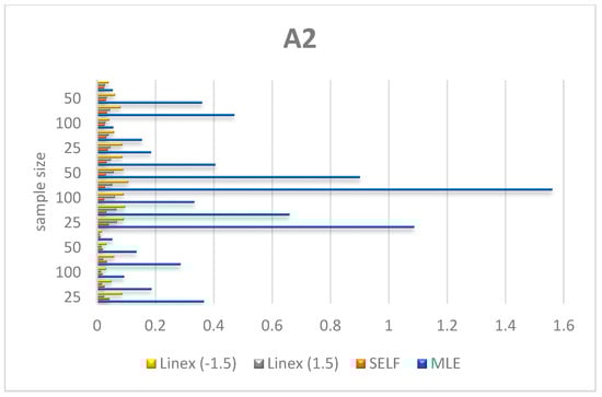
Figure 6. Plot A2 of θ by results in Table 1.

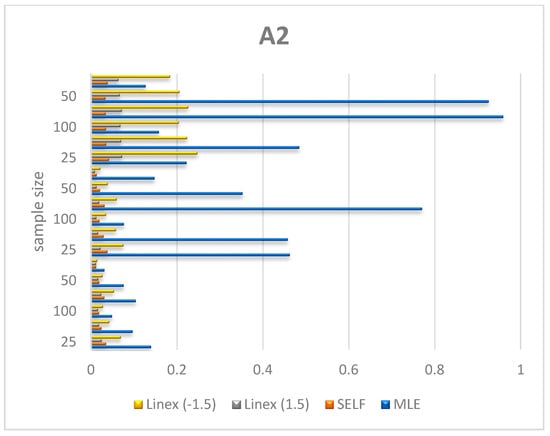
Figure 7. Plot A2 of λ by results in Table 1.

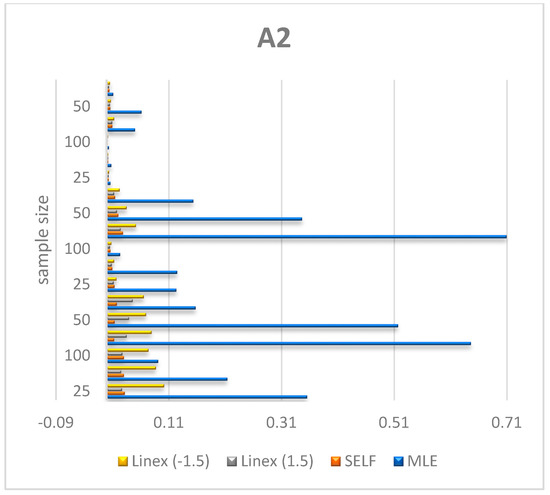
Figure 8. Plot A2 of μ by results in Table 1.

7. Applications

We offer three real-world data applications in this section to demonstrate the significance of the TCPWE, TCPWL, and TCPWR models given in Section 2. We produce the MLEs of the model parameters, as well as goodness-of-fit statistics for any of these models, especially in comparison to those of other competing distributions, such as the Kumaraswamy-generalized Lomax (KGL) distribution, which was introduced by [26]; the Weibull–Lomax (WL), which was introduced by [27]; the Marshall–Olkin alpha power exponential (MOAPE), which was introduced by [4]; the extended odd Weibull exponential (EOWE), which was introduced by [28]; the Exponential Lomax (EL) distribution, which was introduced by [29]; and the Weibull–Rayleigh (WR) distribution, which was introduced by [30]. To compare the fitted models, several measures are taken into account. The Akaike information criterion (AIC), the consistent AIC (CAIC), the Hannan–Quinn information criterion (HQIC), the Bayesian information criterion (BIC), and the accompanying p-value are recommended measurements. The smaller the value of these statistics, the better the match. The results of this models have been shown in Table 4, Table 5 and Table 6.

Table 4. Estimates, SE, goodness-of-fit test by using KS and different criteria measures for strength data.

Models		Estimate	SE	KS	p-Value	AIC	BIC	CAIC	HQIC
TCPWE	θ	2.3783	0.9892	0.0412	0.9998	103.4639	110.1662	103.8331	106.1229
	λ	1.4261	0.9180
	μ	0.3761	0.0641
EOWE	θ	3.2203	0.5172	0.0373	1.0000	103.5728	110.2751	103.9420	106.2319
	λ	0.2541	0.2718
	μ	0.3813	0.0199
MOAPE	θ	55.9197	293.2785	0.0459	0.9987	104.2778	110.9801	104.6470	106.9368
	λ	3.5152	0.3813
	μ	96.3132	144.3345
TCPWL	θ	2.8377	5.6730	0.0413	0.9998	105.4653	114.4017	106.0903	109.0107
	λ	1.2225	2.1030
	α	4.0945	50.6975
	β	10.3516	135.6950
WL	θ	0.9256	0.7027	0.0468	0.9981	105.7308	114.6672	106.3558	109.2761
	λ	0.5624	0.6318
	α	0.0143	0.0158
	β	3.9952	1.6194
KGL	θ	6.2960	0.8903	0.0560	0.9819	106.7560	115.6924	107.3810	110.3013
	λ	2.1020	0.3498
	α	75.7266	2.5650
	β	4.6674	2.0705
EL	θ	17.6259	4.8090	0.1050	0.4326	117.6830	124.3853	118.0522	120.3420
	λ	92.8774	115.6929
	α	45.3783	58.0310
TCPWR	θ	0.7266	0.8309	0.0494	0.9960	103.6717	110.3740	104.0409	106.3307
	λ	2.7926	4.0763
	α	1.2808	0.7316
WR	θ	19.2484	27.7688	0.0541	0.9876	104.1163	110.8186	104.4855	106.7753
	λ	1.7616	0.1786
	α	0.0955	0.0636

Table 5. Estimates, SE, goodness-of-fit test by using KS and different criteria measures for fatigue times.

Models		ESstimate	SE	KS	p-Value	AIC	BIC	CAIC	HQIC
TCPWE	θ	1.7095	0.7385	0.0678	0.7420	918.0491	925.8945	918.2965	921.2252
	λ	7.5045	7.5800
	μ	0.0071	0.0021
EOWE	θ	3.0236	5.0160	0.4987	0.0000	1200.104	1207.949	1200.351	1203.280
	λ	405.1360	298.4960
	μ	0.9993	1.6577
MOAPE	θ	225.6350	202.8139	0.1048	0.2171	928.8386	936.6840	929.0860	932.0146
	λ	0.0603	0.0030
	μ	503.0672	191.5924
TCPWL	θ	0.2180	0.0061	0.0754	0.6134	920.1862	930.6466	920.6028	924.4209
	λ	60.2052	10.7849
	α	51,571.90	15.8489
	β	1,033,343.00	220.2400
WL	θ	0.3111	0.2568	0.0879	0.4165	930.5195	940.9800	930.9362	934.7542
	λ	7.2225	14.3614
	α	0.0041	0.0012
	β	12.2378	8.1955
KGL	θ	64.5972	124.9319	0.0686	0.7294	920.2581	930.7186	920.6747	924.4928
	λ	2.6755	5.7419
	α	29.6256	97.4609
	β	69.1492	275.2303
EL	θ	393.2583	149.6097	0.1080	0.1895	936.2868	944.1322	936.5343	939.4629
	λ	23.7057	8.4717
	α	427.2967	182.3217
TCPWR	θ	0.7207	0.3161	0.0825	0.4978	921.6639	929.5092	921.9113	924.8399
	λ	7.1800	4.1117
	α	81.5052	17.9941
WR	θ	0.0700	0.0151	0.1744	0.0043	984.5768	992.4222	984.8242	987.7529
	λ	0.0091	NA
	α	0.0268	NA

Table 6. Estimates, SE, goodness-of-fit test by using KS and different criteria measures for COVID-19 data.

Models		Estimate	SE	KS	p-value	W*	A*
TCPWL	θ	0.6209	1.0231	0.0603	0.9721	0.0366	0.2655
	λ	2.8853	6.2750
	α	1.1977	1.8145
	β	0.0595	0.0699
TCPWE	θ	0.6793	0.2268	0.1275	0.2439	0.1711	1.0671
	λ	1.3876	0.5961
	μ	5.7589	2.0393
EOWE	θ	1.5284	0.3312	0.0644	0.9449	0.0350	0.2606
	λ	2.2339	1.1390
	μ	12.2319	3.1705
MOAPE	θ	0.0281	0.0448	0.0688	0.9108	0.0614	0.4070
	λ	8.1985	3.2236
	μ	4.7871	3.1396
WL	θ	0.4588	0.3544	0.0692	0.9074	0.0506	0.3384
	λ	0.0152	0.0136
	α	0.4747	0.9199
	β	1.6473	0.5565
KGL	θ	1.8595	0.8224	0.0618	0.9603	0.0369	0.2684
	λ	14.5270	17.2031
	α	0.3996	0.3684
	β	0.4219	0.5482
EL	θ	1.6154	0.4811	0.0617	0.9605	0.0381	0.2748
	λ	5.0903	4.9801
	α	0.3175	0.4248
TCPWR	θ	0.5488	0.1654	0.1671	0.0556	0.2212	1.3786
	λ	0.7289	0.2669
	α	−0.1795	0.0316
WR	θ	9.7459	21.8817	0.0899	0.6651	0.0994	0.6295
	λ	0.5423	0.0617
	α	2.4385	9.1924

7.1. The First Data Set

The first true data set represents the strength of single carbon fibers impregnated at gauge lengths of 1, 10, 20, and 50 mm in GPa. Tows impregnated with 100 fibers were tested at gauge lengths of 20, 50, 150, and 300 mm. The second data set depicts the fatigue times of 6061-T6 aluminum coupons comprising 101 observations with maximum stress per cycle of 31,000 psi. See [4,31]. The numerical values of the AIC, CAIC, BIC, HQIC, A*, W*, and K–S statistics are listed in Table 4. These results show that the TCPWE, TCPWL, and TCPWR models have the lowest KS values and p-values among all fitted models.

7.2. The Second Data Set

The second data set depicts the fatigue times of 6061-T6 aluminum coupons comprising 101 observations with maximum stress per cycle of 31,000 psi. See [4,31]. The numerical values of the AIC, CAIC, BIC, HQIC, A*, W*, and K–S statistics are listed in Table 5. These results show that the TCPWE, TCPWL, and TCPWR models have the lowest KS values and p-values among all fitted models.

Figure 9, Figure 10 and Figure 11 show estimated PDF with histogram, estimated CDF with empirical CDF, P-P plot and Q-Q plot for TCPWE, TCPWL, and TCPWR distributions, which these figures confirmed that the TCPWE, TCPWL, and TCPWR distributions have been fitted for strength data, fatigue times data and COVID-19 data, respectively. To confirm these estimates are maximum, we plot likelihood profile for parameters of TCPWE distribution, where estimate has maximum log-likelihood value, see Figure 12, Figure 13 and Figure 14. To also check existence, we plot the contour plot by two parameters for log-likelihood of the TCPWE distribution, see Figure 15, Figure 16 and Figure 17. We plot likelihood profile for parameters of TCPWL distribution, where the estimate has the maximum log-likelihood value in Figure 18.

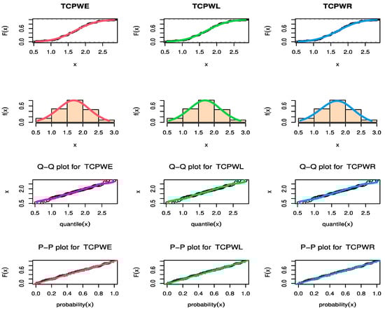
Figure 9. The estimated CDF, fitted PDF, PP-plot, and QQ-plot of the TCPWE and TCPWL and TCPWR distributions for strength data.

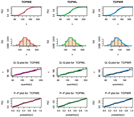
Figure 10. The estimated CDF, fitted PDF, PP-plot, and QQ-plot of the TCPWE and TCPWL and TCPWR distributions for fatigue times.

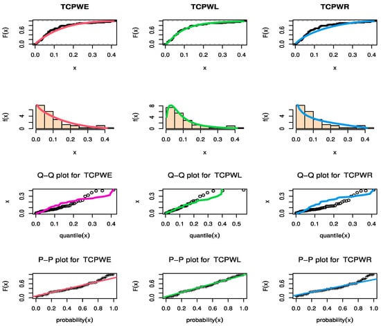
Figure 11. The estimated CDF, fitted PDF, PP-plot, and QQ-plot of the TCPWE, TCPWL, and TCPWR distributions for COVID-19 data.

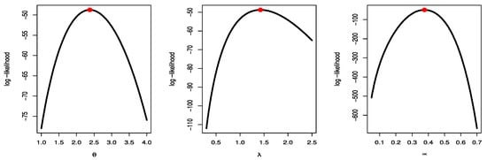
Figure 12. Likelihood profile for parameters of TCPWE distribution for strength data.

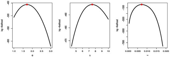
Figure 13. Likelihood profile for parameters of TCPWE distribution for fatigue times.

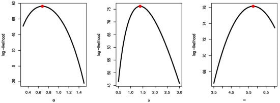
Figure 14. Likelihood profile for parameters of TCPWE distribution for COVID-19 data.

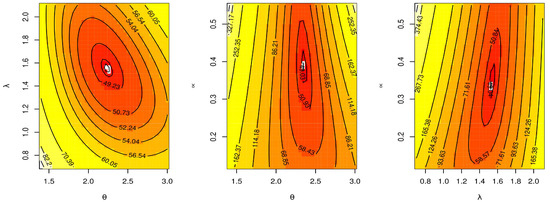
Figure 15. Contour plot for log-likelihood of the TCPWE distribution for strength data.

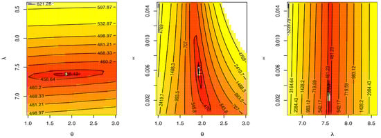
Figure 16. Contour plot for log-likelihood of the TCPWE distribution for fatigue times.

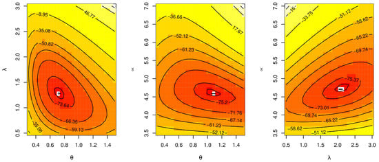
Figure 17. Contour plot for log-likelihood of the TCPWE distribution for COVID-19 data.

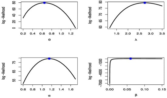
Figure 18. Likelihood profile for parameters of TCPWL distribution for COVID-19 data.

7.3. The Third Data Set

The third data set represents the COVID-19 data from the United Kingdom within 62 days, from 21 July to 21 August 2020. These data describe the drought mortality rate as follows: 0.2992, 0.1303, 0.0587, 0.3926, 0.3622, 0.4110, 0.3188, 0.1652, 0.1277, 0.0863, 0.2173, 0.3969, 0.1673, 0.1995, 0.1300, 0.0771, 0.0445, 0.2180, 0.2296, 0.1246, 0.1362, 0.0680, 0.0359, 0.0399, 0.1749, 0.1031, 0.0949, 0.1025, 0.0354, 0.0432, 0.0392, 0.0977, 0.0662, 0.0350, 0.1240, 0.0580, 0.0309, 0.0116, 0.0809, 0.1229, 0.0077, 0.0763, 0.0495, 0.0190, 0.0038, 0.0679, 0.0526, 0.0674, 0.0448, 0.0112, 0.0185, 0.0666, 0.0479, 0.0734, 0.0658, 0.0400, 0.0109, 0.0180, 0.0108, 0.0430, 0.0572, 0.0214.

8. Conclusions

This article formulated a new family that has more attractive and flexible distributions and greatly improves the modelling ability of their baseline distributions in the description of real-life events such as carbon and COVID-19 data. A new, flexible extension to the odd Weibull-G family based on a truncated Cauchy power generator was provided. Based on Truncated Cauchy Power Weibull and some classic distribution baselines such as Lomax, exponential, and Rayleigh distributions, this paper introduced three new distributions. Some statistical properties of the new family were provided. Complete and censored samples were considered under this model. In censored samples, the greater the number of censored sample units, the lower the MSE and the bias. Bayesian and MLE methods of estimation were also considered. LINEX and SE loss functions were deduced for Bayesian estimators based on different loss functions. A Monte Carlo simulation study was designed to assess the performance of estimates. Generally, we concluded that the Bayesian estimates are preferable to the corresponding other estimates in most of the situations. A new distribution based on the Lomax distribution was the best model to fit different data sets such as those for carbon fibers and COVID-19.

References

- Eugene, N.; Lee, C.; Famoye, F. Beta-normal distribution and its applications. Commun. Stat. Theory Methods 2002, 31, 497–512. [Google Scholar] [CrossRef]
- Zografos, K.; Balakrishnan, N. On the families of beta-and gamma-generated generalized distribution and associated inference. Stat. Methodol. 2009, 6, 344–362. [Google Scholar] [CrossRef]
- Cordeiro, G.M.; de Castro, M. A new family of generalized distributions. J. Stat. Comput. Simul. 2012, 81, 883–893. [Google Scholar] [CrossRef]
- Nassar, M.; Kumar, D.; Dey, S.; Cordeiro, G.M.; Afify, A.Z. The Marshall–Olkin alpha power family of distributions with applications. J. Comput. Appl. Math. 2019, 351, 41–53. [Google Scholar] [CrossRef]
- Cordeiro, G.M.; Afify, A.Z.; Ortega, E.M.; Suzuki, A.K.; Mead, M.E. The odd Lomax generator of distributions: Properties, estimation and applications. J. Comput. Appl. Math. 2019, 347, 222–237. [Google Scholar] [CrossRef]
- Hassan, S.A.; Elgarhy, M. Type II half logistic family of distributions with Applications. Pak. J. Stat. Oper. Res. 2017, 13, 245–264. [Google Scholar]
- Badr, M.M.; Elbatal, I.; Jamal, F.; Chesneau, C.; Elgarhy, M. The transmuted odd Fréchet-G family of distributions: Theory and applications. Mathematics 2020, 8, 958. [Google Scholar] [CrossRef]
- Al-Mofleh, H.; Elgarhy, M.; Afify, A.Z.; Zannon, M.S. Type II exponentiated half logistic generated family of distributions with applications. Electron. J. Appl. Stat. Anal. 2020, 13, 536–561. [Google Scholar]
- Bantan, R.A.; Chesneau, C.; Jamal, F.; Elgarhy, M. On the analysis of new COVID-19 cases in Pakistan using an exponentiated version of the M family of distributions. Mathematics 2020, 8, 953. [Google Scholar] [CrossRef]
- Almarashi, A.M.; Jamal, F.; Chesneau, C.; Elgarhy, M. The Exponentiated truncated inverse Weibull-generated Ffamily of distributions with applications. Symmetry 2020, 12, 650. [Google Scholar] [CrossRef]
- Bourguignon, M.; Silva, R.B.; Cordeiro, G.M. The Weibull-G family of probability distributions. J. Data Sci. 2014, 12, 1253–1268. [Google Scholar] [CrossRef]
- Nadarajah, S.; Kotz, S. A truncated Cauchy distribution. Int. J. Math. Educ. Sci. Technol. 2006, 37, 605–608. [Google Scholar] [CrossRef]
- Hamedani, G.; Ghosh, I. Kumaraswamy-Half-Cauchy Distribution: Characterizations and Related Results. Int. J. Stat. Probab. 2015, 4, 94–100. [Google Scholar] [CrossRef][Green Version]
- Zubair, M.; Tahir, M.; Cordeiro, M.; Alzaatreh, A.; Ortega, M. The power-Cauchy negative-binomial: Properties and regression. J. Stat. Distrib. Appl. 2018, 5, 1–17. [Google Scholar] [CrossRef]
- Aldahlan, M.A.; Jamal, F.; Chesneau, C.; Elgarhy, M.; Elbatal, I. The truncated Cauchy power family of distributions with inference and applications. Entropy 2020, 22, 346. [Google Scholar] [CrossRef] [PubMed]
- Almetwally, E.M.; Almongy, H.M.; Mubarak, A. Bayesian and maximum likelihood estimation for the Weibull generalized exponential distribution parameters using progressive censoring schemes. Pak. J. Stat. Oper. Res. 2018, 14, 853–868. [Google Scholar] [CrossRef]
- Ahmad, H.H.; Almetwally, E. Marshall-Olkin generalized Pareto distribution: Bayesian and non Bayesian estimation. Pak. J. Stat. Oper. Res. 2020, 16, 21–33. [Google Scholar] [CrossRef]
- Nassar, M.; Abo-Kasem, O.; Zhang, C.; Dey, S. Analysis of Weibull Distribution Under Adaptive Type-II Progressive Hybrid Censoring Scheme. J. Indian Soc. Probab. Stat. 2018, 19, 25–65. [Google Scholar] [CrossRef]
- Dey, S.; Singh, S.; Tripathi, Y.M.; Asgharzadeh, A. Estimation and prediction for a progressively censored generalized inverted exponential distribution. Stat. Methodol. 2016, 32, 185–202. [Google Scholar] [CrossRef]
- Kundu, D.; Pradhan, B. Estimating the parameters of the generalized exponential distribution in presence of hybrid censoring. Commun. Stat.-Theory Methods 2009, 38, 2030–2041. [Google Scholar] [CrossRef]
- Balakrishnan, N.; Aggarwala, R. Progressive Censoring: Theory, Methods, and Applications; Springer Science Business Media: Berlin/Heidelberg, Germany, 2000. [Google Scholar]
- El-Morshedy, M.; Eliwa, M.S.; El-Gohary, A.; Almetwally, E.M.; L-Desokey, R.E. Exponentiated generalized inverse flexible Weibull distribution: Bayesian and non-Bayesian estimation under complete and type II censored samples with applications. Commun. Math. Stat. 2021, 4, 1–22. [Google Scholar] [CrossRef]
- Almongy, H.M.; Almetwally, E.M.; Alharbi, R.; Alnagar, D.; Hafez, E.H.; El-Din, M.M.M. The Weibull generalized exponential distribution with censored sample: Estimation and application on real data. Complexity 2021, 2021, 6653534. [Google Scholar] [CrossRef]
- El-Raheem, A.M.A.; Almetwally, E.M.; Mohamed, M.S.; Hafez, E.H. Accelerated life tests for modified Kies exponential lifetime distribution: Binomial removal, transformers turn insulation application and numerical results. AIMS Math. 2021, 6, 5222–5255. [Google Scholar] [CrossRef]
- Bantan, R.; Hassan, A.S.; Almetwally, E.; Elgarhy, M.; Jamal, F.; Chesneau, C.; Elsehetry, M. Bayesian analysis in partially accelerated life tests for weighted Lomax distribution. Comput. Mater. Contin. 2021, 68, 2859–2875. [Google Scholar] [CrossRef]
- Shams, T.M. The Kumaraswamy-generalized Lomax distribution. Middle-East J. Sci. Res. 2013, 17, 641–646. [Google Scholar]
- Tahir, M.H.; Cordeiro, G.M.; Mansoor, M.; Zubair, M. The Weibull-Lomax distribution: Properties and applications. Hacet. J. Math. Stat. 2015, 44, 461–480. [Google Scholar] [CrossRef]
- Afify, A.Z.; Mohamed, O.A. A new three-parameter exponential distribution with variable shapes for the hazard rate: Estimation and applications. Mathematics 2020, 8, 135. [Google Scholar] [CrossRef]
- El-Bassiouny, A.H.; Abdo, N.F.; Shahen, H.S. Exponential Lomax distribution. Int. J. Comput. Appl. 2015, 121, 24–29. [Google Scholar]
- Merovci, F.; Elbatal, I. Weibull-Rayleigh distribution: Theory and applications. Appl. Math. Inf. Sci. 2015, 9, 1–11. [Google Scholar]
- Birnbaum, Z.W.; Saunders, S.C. Estimation for a family of life distributions with applications to fatigue. J. Appl. Probab. 1969, 6, 328–347. [Google Scholar] [CrossRef]
Publisher’s Note: MDPI stays neutral with regard to jurisdictional claims in published maps and institutional affiliations. |
© 2022 by the authors. Licensee MDPI, Basel, Switzerland. This article is an open access article distributed under the terms and conditions of the Creative Commons Attribution (CC BY) license (https://creativecommons.org/licenses/by/4.0/).