
Knacks of Fractional Order Swarming Intelligence for Parameter Estimation of Harmonics in Electrical Systems

 , , and
Abstract
:1. Introduction
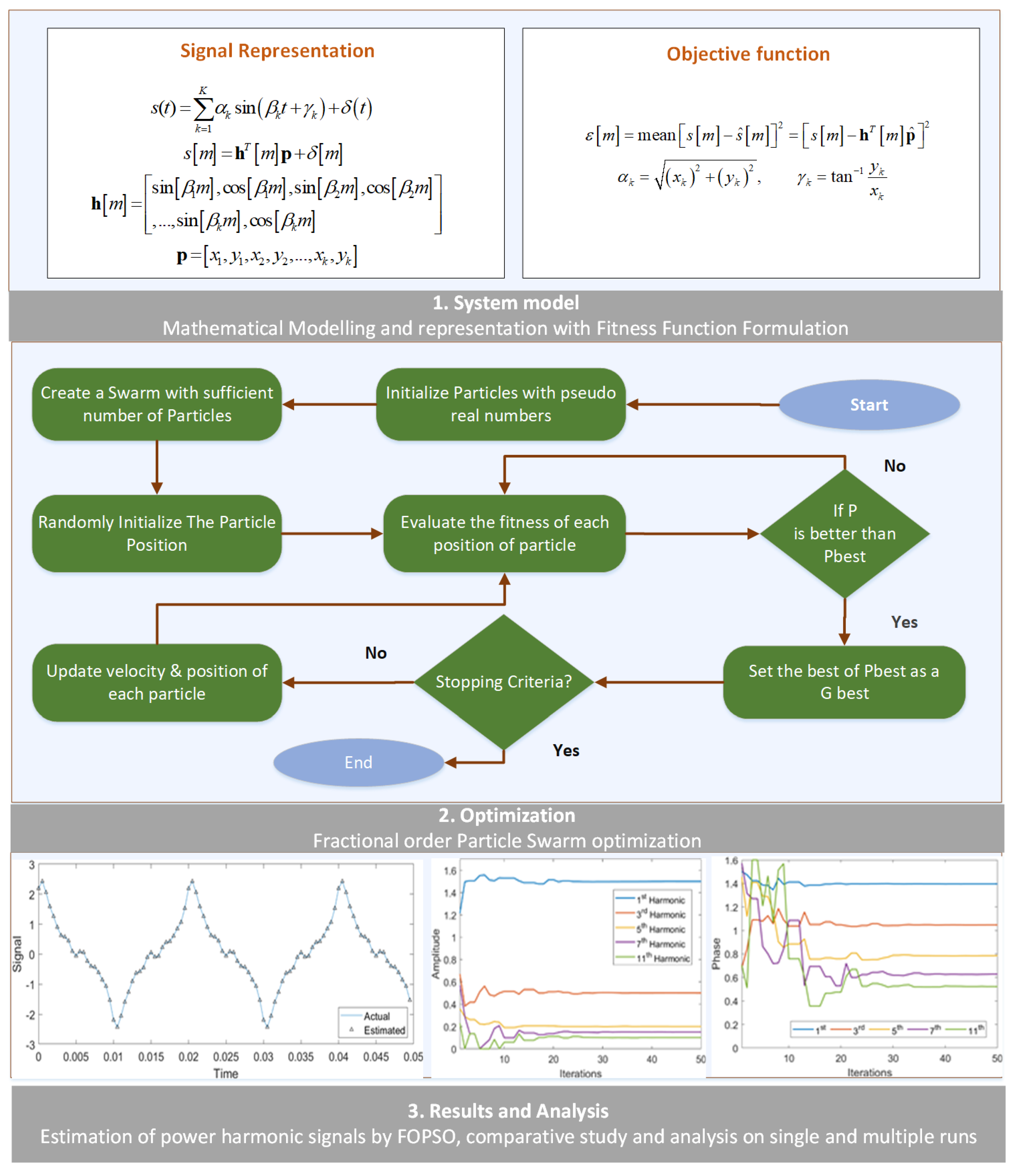
- A fractional order swarming optimization approach exploiting the inherited legacy of the fractional calculus is presented for the nonlinear parameter estimation problem of electrical harmonics.
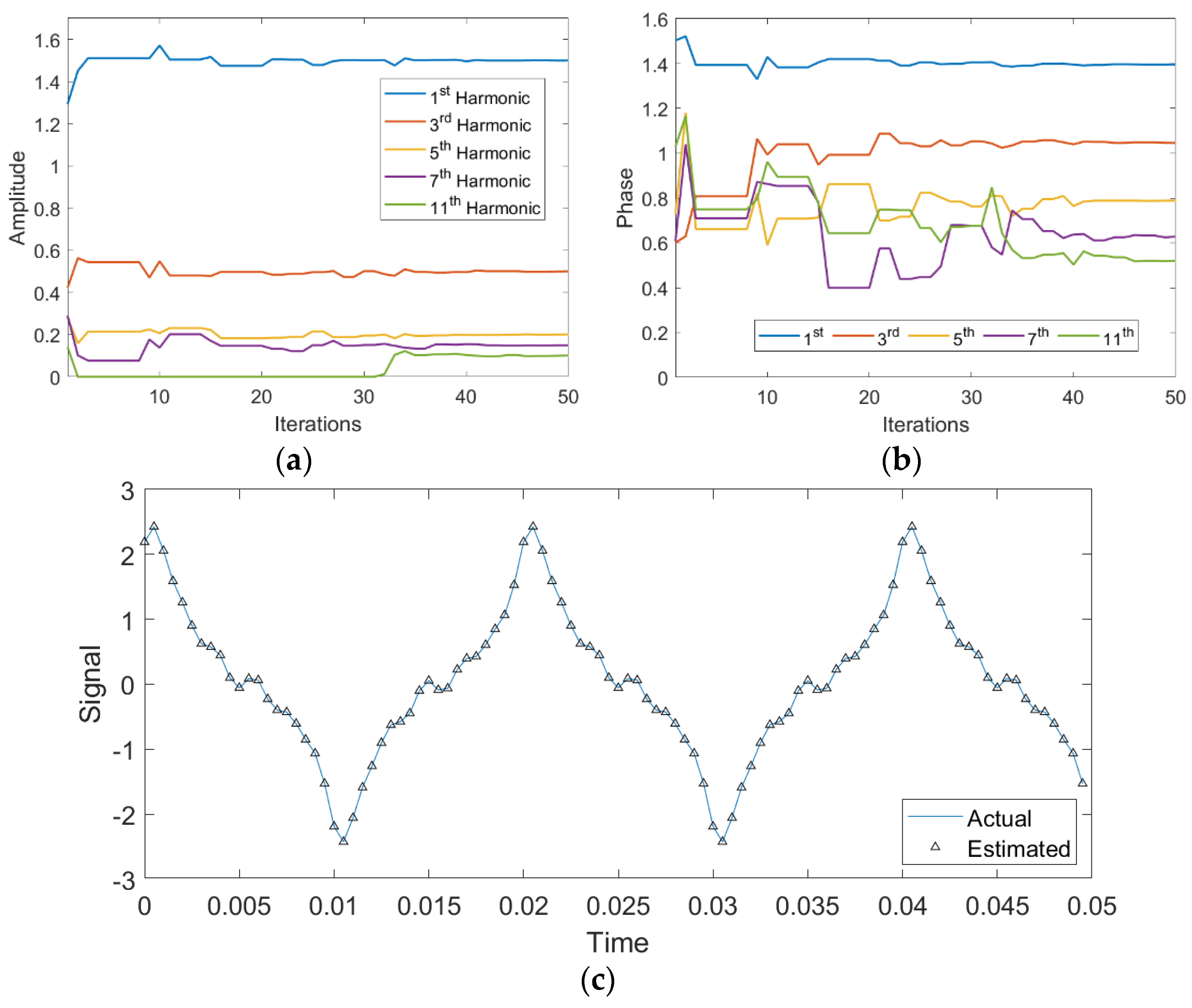
- The proposed fractional order particle swarm optimization (FOPSO) effectively estimates the amplitude and phase parameters of the harmonic signal compared with the standard counterpart for different scenarios of additive white Gaussian noise.
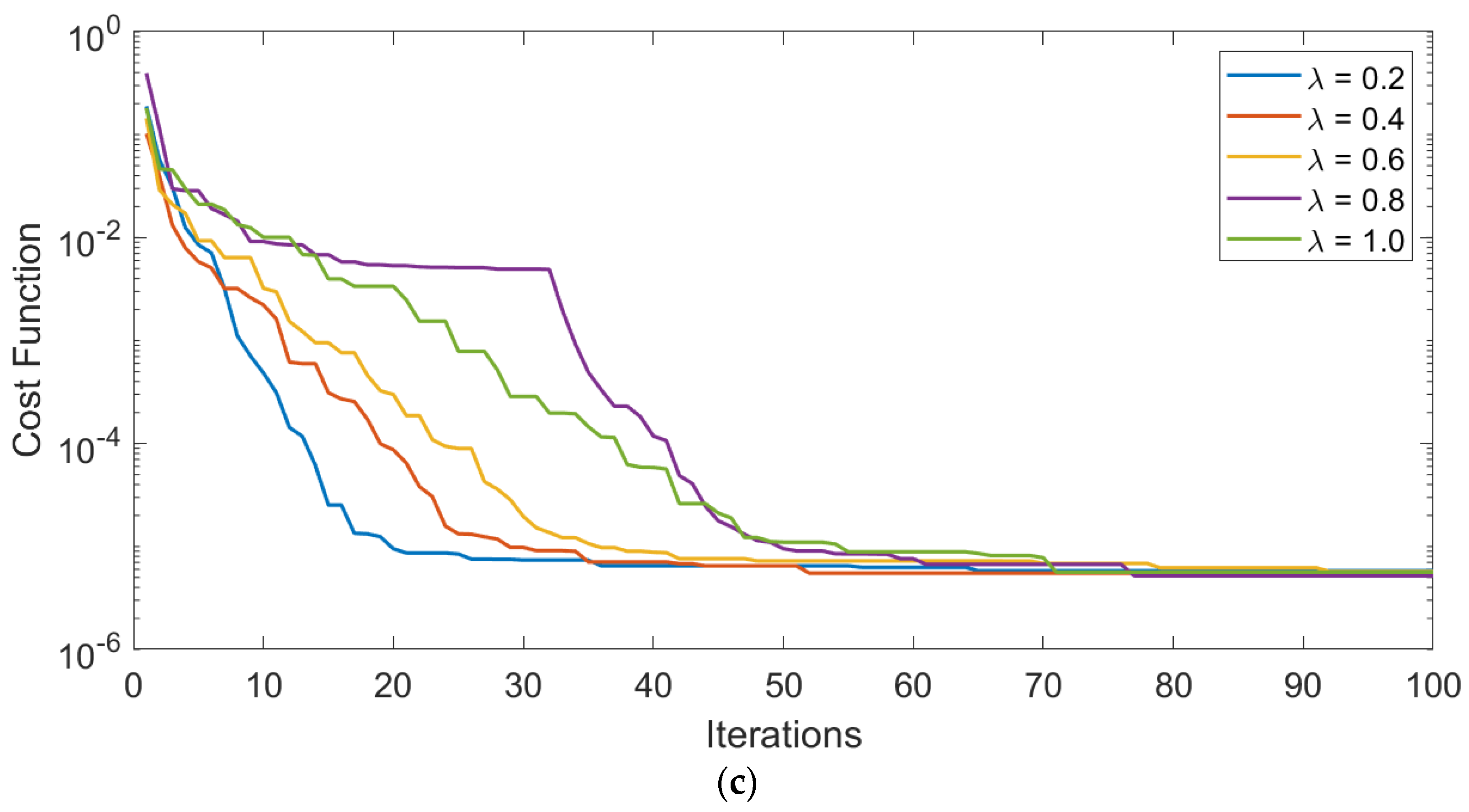
- The best convergence performance of the FOPSO is obtained for a fractional order of 0.1 that reduces gradually with increase in the fractional order until unity (standard PSO).
- The reliability analyses, through autonomous executions of the FOPSO for harmonics parameter identification, confirm superior performance in the case of a fractional order of 0.1 for all noise variations.
2. Harmonics Identification Model
3. Methodology
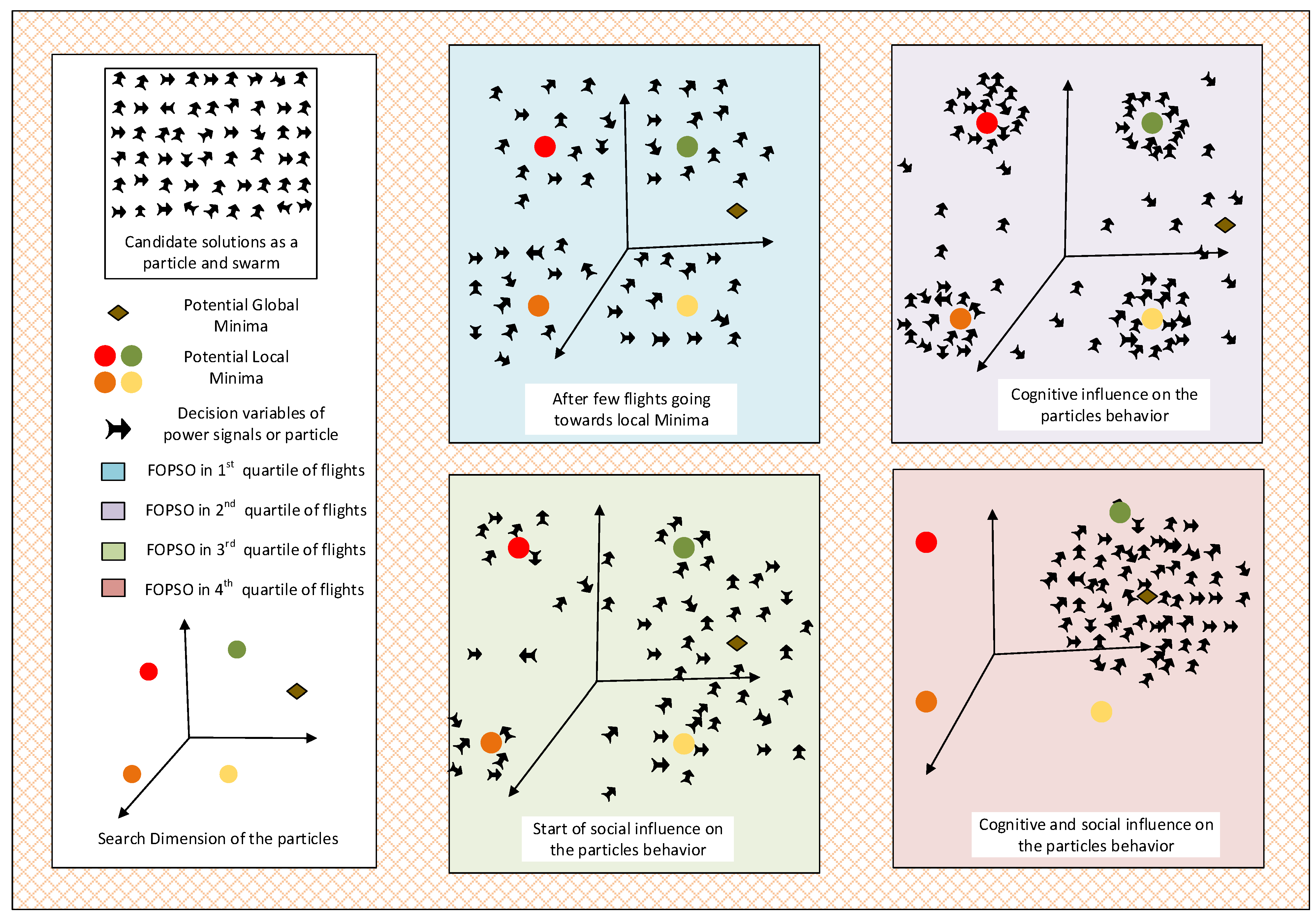
Optimization Procedure: Fractional Swarming Computing Paradigm
| Algorithm 1. Pseudocode for FOPSO to solve the harmonics identification model |
|
4. Results and Discussion
5. Conclusions
Supplementary Materials
Author Contributions
Funding
Conflicts of Interest
References
- Van Der Heijden, F.; Duin, R.P.; De Ridder, D.; Tax, D.M. Classification, Parameter Estimation and State Estimation: An Engineering Approach Using MATLAB; John Wiley & Sons: Hoboken, NJ, USA, 2005. [Google Scholar]
- Silvey, S. Optimal Design: An Introduction to the Theory for Parameter Estimation; Springer Science & Business Media: Berlin, Germany, 2013; Volume 1. [Google Scholar]
- Mehmood, A.; Zameer, A.; Chaudhary, N.I.; Ling, S.H.; Raja, M.A.Z. Design of meta-heuristic computing paradigms for Hammerstein identification systems in electrically stimulated muscle models. Neural Comput. Appl. 2020, 32, 12469–12497. [Google Scholar] [CrossRef]
- Raja, M.A.Z.; Shah, A.A.; Mehmood, A.; Chaudhary, N.I.; Aslam, M.S. Bio-inspired computational heuristics for parameter estimation of nonlinear Hammerstein controlled autoregressive system. Neural Comput. Appl. 2018, 29, 1455–1474. [Google Scholar] [CrossRef]
- Yang, X.; Yang, Y.; Liu, Y.; Deng, Z. A reliability assessment approach for electric power systems considering wind power uncertainty. IEEE Access 2020, 8, 12467–12478. [Google Scholar] [CrossRef]
- Beleiu, H.G.; Maier, V.; Pavel, S.G.; Birou, I.; Pică, C.S.; Dărab, P.C. Harmonics consequences on drive systems with induction motor. Appl. Sci. 2020, 10, 1528. [Google Scholar] [CrossRef] [Green Version]
- Almutairi, M.S.; Hadjiloucas, S. Harmonics mitigation based on the minimization of non-linearity current in a power system. Designs 2019, 3, 29. [Google Scholar] [CrossRef] [Green Version]
- Phannil, N.; Jettanasen, C.; Ngaopitakkul, A. Harmonics and reduction of energy consumption in lighting systems by using LED lamps. Energies 2018, 11, 3169. [Google Scholar] [CrossRef] [Green Version]
- Singh, S.K.; Sinha, N.; Goswami, A.K.; Sinha, N. Several variants of Kalman Filter algorithm for power system harmonic estimation. Int. J. Electr. Power Energy Syst. 2016, 78, 793–800. [Google Scholar] [CrossRef]
- Joorabian, M.; Mortazavi, S.S.; Khayyami, A.A. Harmonic estimation in a power system using a novel hybrid Least Squares-Adaline algorithm. Electr. Power Syst. Res. 2009, 79, 107–116. [Google Scholar] [CrossRef]
- Enayati, J.; Moravej, Z. Real-time harmonics estimation in power systems using a novel hybrid algorithm. IET Gener. Transm. Distrib. 2017, 11, 3532–3538. [Google Scholar] [CrossRef]
- Sarkar, A.; Choudhury, S.R.; Sengupta, S. A self-synchronized ADALINE network for on-line tracking of power system harmonics. Measurement 2011, 44, 784–790. [Google Scholar] [CrossRef]
- Liu, S.; Ding, F.; Xu, L.; Hayat, T. Hierarchical principle-based iterative parameter estimation algorithm for dual-frequency signals. Circuits Syst. Signal Process. 2019, 38, 3251–3268. [Google Scholar] [CrossRef]
- Xu, L.; Chen, F.; Ding, F.; Alsaedi, A.; Hayat, T. Hierarchical recursive signal modeling for multifrequency signals based on discrete measured data. Int. J. Adapt. Control Signal Process. 2021, 35, 676–693. [Google Scholar] [CrossRef]
- Xu, L.; Ding, F.; Zhu, Q. Separable synchronous multi-innovation gradient-based iterative signal modeling from on-line measurements. IEEE Trans. Instrum. Meas. 2022, 71, 6501313. [Google Scholar] [CrossRef]
- Mirjalili, S.; Faris, H.; Aljarah, I. Evolutionary Machine Learning Techniques; Springer: Singapore, 2019. [Google Scholar]
- Mohammadian, M.; Lorestani, A.; Ardehali, M.M. Optimization of single and multi-areas economic dispatch problems based on evolutionary particle swarm optimization algorithm. Energy 2018, 161, 710–724. [Google Scholar] [CrossRef]
- Mehmood, A.; Raja, M.A.Z.; Shi, P.; Chaudhary, N.I. Weighted differential evolution-based heuristic computing for identification of Hammerstein systems in electrically stimulated muscle modeling. Soft Comput. 2022, 1–17. [Google Scholar] [CrossRef]
- Ray, P.K.; Subudhi, B. BFO optimized RLS algorithm for power system harmonics estimation. Appl. Soft Comput. 2012, 12, 1965–1977. [Google Scholar] [CrossRef]
- Mehmood, A.; Chaudhary, N.I.; Raja, M.A.Z. Novel computing paradigms for parameter estimation in power signal models. Neural Comput. Appl. 2020, 32, 6253–6282. [Google Scholar] [CrossRef]
- Mehmood, A.; Shi, P.; Raja, M.A.Z.; Zameer, A.; Chaudhary, N.I. Design of backtracking search heuristics for parameter estimation of power signals. Neural Comput. Appl. 2021, 33, 1479–1496. [Google Scholar] [CrossRef]
- Elvira-Ortiz, D.A.; Jaen-Cuellar, A.Y.; Morinigo-Sotelo, D.; Morales-Velazquez, L.; Osornio-Rios, R.A.; Romero-Troncoso, R.d.J. Genetic algorithm methodology for the estimation of generated power and harmonic content in photovoltaic generation. Appl. Sci. 2020, 10, 542. [Google Scholar] [CrossRef] [Green Version]
- do Nascimento Sepulchro, W.; Encarnação, L.F.; Brunoro, M. Harmonic state and power flow estimation in distribution systems using evolutionary strategy. J. Control Autom. Electr. Syst. 2014, 25, 358–367. [Google Scholar] [CrossRef]
- Subramaniyan, S.; Ramiah, J. Improved football game optimization for state estimation and power quality enhancement. Comput. Electr. Eng. 2020, 81, 106547. [Google Scholar] [CrossRef]
- Singh, S.K.; Sinha, N.; Goswami, A.K.; Sinha, N. Robust estimation of power system harmonics using a hybrid firefly based recursive least square algorithm. Int. J. Electr. Power Energy Syst. 2016, 80, 287–296. [Google Scholar] [CrossRef]
- Kabalci, Y.; Kockanat, S.; Kabalci, E. A modified ABC algorithm approach for power system harmonic estimation problems. Electr. Power Syst. Res. 2018, 154, 160–173. [Google Scholar] [CrossRef]
- Yu, Z.; Sun, G.; Lv, J. A fractional-order momentum optimization approach of deep neural networks. Neural Comput. Appl. 2022, 34, 7091–7111. [Google Scholar] [CrossRef]
- Chaudhary, N.I.; Raja, M.A.Z.; Khan, Z.A.; Mehmood, A.; Shah, S.M. Design of fractional hierarchical gradient descent algorithm for parameter estimation of nonlinear control autoregressive systems. Chaos Solitons Fractals 2022, 157, 111913. [Google Scholar] [CrossRef]
- Machado, J.T.; Kiryakova, V.; Mainardi, F. Recent history of fractional calculus. Commun. Nonlinear Sci. Numer. Simul. 2011, 16, 1140–1153. [Google Scholar] [CrossRef] [Green Version]
- Akdemir, A.O.; Butt, S.I.; Nadeem, M.; Ragusa, M.A. New general variants of Chebyshev type inequalities via generalized fractional integral operators. Mathematics 2021, 9, 122. [Google Scholar] [CrossRef]
- Liu, X.; Bo, Y.; Jin, Y. A Numerical Method for the Variable-Order Time-Fractional Wave Equations Based on the H2N2 Approximation. J. Funct. Spaces 2022, 2022, 3438289. [Google Scholar] [CrossRef]
- Khan, Z.A.; Chaudhary, N.I.; Zubair, S. Fractional stochastic gradient descent for recommender systems. Electron. Mark. 2019, 29, 275–285. [Google Scholar] [CrossRef]
- Khan, Z.A.; Zubair, S.; Chaudhary, N.I.; Raja, M.A.Z.; Khan, F.A.; Dedovic, N. Design of normalized fractional SGD computing paradigm for recommender systems. Neural Comput. Appl. 2020, 32, 10245–10262. [Google Scholar] [CrossRef]
- Yousri, D.; Mirjalili, S. Fractional-order cuckoo search algorithm for parameter identification of the fractional-order chaotic, chaotic with noise and hyper-chaotic financial systems. Eng. Appl. Artif. Intell. 2020, 92, 103662. [Google Scholar] [CrossRef]
- Yousri, D.; Abd Elaziz, M.; Mirjalili, S. Fractional-order calculus-based flower pollination algorithm with local search for global optimization and image segmentation. Knowl.-Based Syst. 2020, 197, 105889. [Google Scholar] [CrossRef]
- Yousri, D.; Mirjalili, S.; Machado, J.T.; Thanikanti, S.B.; Fathy, A. Efficient fractional-order modified Harris Hawks optimizer for proton exchange membrane fuel cell modeling. Eng. Appl. Artif. Intell. 2021, 100, 104193. [Google Scholar] [CrossRef]
- Chaudhary, N.I.; Zubair, S.; Raja, M.A.Z. A new computing approach for power signal modeling using fractional adaptive algorithms. ISA Trans. 2017, 68, 189–202. [Google Scholar] [CrossRef] [PubMed]
- Zubair, S.; Chaudhary, N.I.; Khan, Z.A.; Wang, W. Momentum fractional LMS for power signal parameter estimation. Signal Process. 2018, 142, 441–449. [Google Scholar] [CrossRef]
- Chaudhary, N.I.; Latif, R.; Raja, M.A.Z.; Machado, J.T. An innovative fractional order LMS algorithm for power signal parameter estimation. Appl. Math. Model. 2020, 83, 703–718. [Google Scholar] [CrossRef]
- Pires, E.J.S.; Machado, J.A.T.; Oliveira, P.B.M.; Cunha, J.B.; Mendes, L. Particle swarm optimization with fractional-order velocity. Nonlinear Dyn. 2010, 61, 295–301. [Google Scholar] [CrossRef] [Green Version]
- Couceiro, M.S.; Rocha, R.P.; Ferreira, N.M.; Machado, J.A. Introducing the fractional-order Darwinian PSO. Signal Image Video Process. 2012, 6, 343–350. [Google Scholar] [CrossRef] [Green Version]
- Ghamisi, P.; Couceiro, M.S.; Martins, F.M.; Benediktsson, J.A. Multilevel image segmentation based on fractional-order Darwinian particle swarm optimization. IEEE Trans. Geosci. Remote Sens. 2013, 52, 2382–2394. [Google Scholar] [CrossRef] [Green Version]
- Shahri, E.S.A.; Alfi, A.; Machado, J.T. Fractional fixed-structure H∞ controller design using augmented Lagrangian particle swarm optimization with fractional order velocity. Appl. Soft Comput. 2019, 77, 688–695. [Google Scholar] [CrossRef]
- Pahnehkolaei, S.M.A.; Alfi, A.; Machado, J.T. Analytical stability analysis of the fractional-order particle swarm optimization algorithm. Chaos Solitons Fractals 2022, 155, 111658. [Google Scholar] [CrossRef]
- Zameer, A.; Muneeb, M.; Mirza, S.M.; Raja, M.A.Z. Fractional-order particle swarm based multi-objective PWR core loading pattern optimization. Ann. Nucl. Energy 2020, 135, 106982. [Google Scholar] [CrossRef]
- Khan, M.W.; Muhammad, Y.; Raja, M.A.Z.; Ullah, F.; Chaudhary, N.I.; He, Y. A new fractional particle swarm optimization with entropy diversity based velocity for reactive power planning. Entropy 2020, 22, 1112. [Google Scholar] [CrossRef]
- Muhammad, Y.; Khan, R.; Raja, M.A.Z.; Ullah, F.; Chaudhary, N.I.; He, Y. Design of fractional swarm intelligent computing with entropy evolution for optimal power flow problems. IEEE Access 2020, 8, 111401–111419. [Google Scholar] [CrossRef]
- Sabatier, J.A.T.M.J.; Agrawal, O.P.; Machado, J.T. Advances in Fractional Calculus; Springer: Dordrecht, The Netherlands, 2007; Volume 4, p. 9. [Google Scholar]
- Teodoro, G.S.; Machado, J.T.; De Oliveira, E.C. A review of definitions of fractional derivatives and other operators. J. Comput. Phys. 2019, 388, 195–208. [Google Scholar] [CrossRef]
- Couceiro, M.; Ghamisi, P. Fractional Order Darwinian Particle Swarm Optimization Applications and Evaluation of An Evolutionary Algorithm; Springer: Berlin, Germany, 2016; ISBN 978-3-319-19634-3. [Google Scholar]
- Chen, J.; Ma, J.; Gan, M.; Zhu, Q. Multi-direction gradient iterative algorithm: A unified framework for gradient iterative and least squares algorithms. IEEE Trans. Autom. Control 2021. [Google Scholar] [CrossRef]
- Chen, J.; Ding, F.; Zhu, Q.; Liu, Y. Interval error correction auxiliary model based gradient iterative algorithms for multirate ARX models. IEEE Trans. Autom. Control 2019, 65, 4385–4392. [Google Scholar] [CrossRef]
- Xu, L.; Ding, F.; Yang, E. Auxiliary model multiinnovation stochastic gradient parameter estimation methods for nonlinear sandwich systems. Int. J. Robust Nonlinear Control 2021, 31, 148–165. [Google Scholar] [CrossRef]
- Xu, L.; Ding, F.; Zhu, Q. Decomposition strategy-based hierarchical least mean square algorithm for control systems from the impulse responses. Int. J. Syst. Sci. 2021, 52, 1806–1821. [Google Scholar] [CrossRef]


| δ | t | α1 | α2 | α3 | α4 | α5 | γ1 | γ2 | γ3 | γ4 | γ5 | ε |
| 200 | 10 | 1.3877 | 0.4372 | 0.3642 | 0.3479 | 0.3401 | 1.5774 | 1.2000 | 1.4482 | 1.2608 | 0.4896 | 1.32 × 10⁻¹ |
| 20 | 1.4907 | 0.4986 | 0.2045 | 0.1439 | 0.1062 | 1.3967 | 1.0491 | 0.7894 | 0.6153 | 0.5417 | 9.76 × 10⁻⁵ | |
| 30 | 1.5000 | 0.5001 | 0.1998 | 0.1499 | 0.0998 | 1.3962 | 1.0466 | 0.7853 | 0.6287 | 0.5228 | 1.24 × 10⁻⁷ | |
| 40 | 1.5000 | 0.5000 | 0.2000 | 0.1500 | 0.1000 | 1.3960 | 1.0470 | 0.7850 | 0.6280 | 0.5229 | 1.12 × 10⁻¹⁰ | |
| 50 | 1.5000 | 0.5000 | 0.2000 | 0.1500 | 0.1000 | 1.3960 | 1.0470 | 0.7850 | 0.6280 | 0.5230 | 2.51 × 10⁻¹³ | |
| 60 | 1.5000 | 0.5000 | 0.2000 | 0.1500 | 0.1000 | 1.3960 | 1.0470 | 0.7850 | 0.6280 | 0.5230 | 7.46 × 10⁻¹⁷ | |
| 70 | 1.5000 | 0.5000 | 0.2000 | 0.1500 | 0.1000 | 1.3960 | 1.0470 | 0.7850 | 0.6280 | 0.5230 | 8.40 × 10⁻²⁰ | |
| 80 | 1.5000 | 0.5000 | 0.2000 | 0.1500 | 0.1000 | 1.3960 | 1.0470 | 0.7850 | 0.6280 | 0.5230 | 8.05 × 10⁻²¹ | |
| 90 | 1.5000 | 0.5000 | 0.2000 | 0.1500 | 0.1000 | 1.3960 | 1.0470 | 0.7850 | 0.6280 | 0.5230 | 7.90 × 10⁻²¹ | |
| 100 | 1.5000 | 0.5000 | 0.2000 | 0.1500 | 0.1000 | 1.3960 | 1.0470 | 0.7850 | 0.6280 | 0.5230 | 6.43 × 10⁻²¹ | |
| 70 | 10 | 1.2489 | 0.7684 | 0.1411 | 0.1246 | 0.3677 | 0.9979 | 0.6191 | 1.3253 | 1.2996 | 1.1829 | 3.02 × 10⁻¹ |
| 20 | 1.4961 | 0.5006 | 0.1952 | 0.1432 | 0.1041 | 1.3980 | 1.0495 | 0.8365 | 0.6433 | 0.5207 | 1.11 × 10⁻⁴ | |
| 30 | 1.5000 | 0.5001 | 0.1997 | 0.1500 | 0.1000 | 1.3960 | 1.0470 | 0.7860 | 0.6279 | 0.5258 | 1.75 × 10⁻⁷ | |
| 40 | 1.4999 | 0.5001 | 0.1998 | 0.1501 | 0.1001 | 1.3960 | 1.0471 | 0.7849 | 0.6278 | 0.5238 | 9.86 × 10⁻⁸ | |
| 50 | 1.4999 | 0.5000 | 0.1999 | 0.1500 | 0.1000 | 1.3960 | 1.0470 | 0.7850 | 0.6277 | 0.5236 | 7.05 × 10⁻⁸ | |
| 60 | 1.4999 | 0.5000 | 0.1999 | 0.1500 | 0.1000 | 1.3960 | 1.0470 | 0.7850 | 0.6277 | 0.5236 | 7.05 × 10⁻⁸ | |
| 70 | 1.4999 | 0.5000 | 0.1999 | 0.1500 | 0.1000 | 1.3960 | 1.0471 | 0.7850 | 0.6277 | 0.5236 | 6.76 × 10⁻⁸ | |
| 80 | 1.4999 | 0.5000 | 0.1999 | 0.1500 | 0.1000 | 1.3960 | 1.0471 | 0.7850 | 0.6277 | 0.5236 | 6.76 × 10⁻⁸ | |
| 90 | 1.5000 | 0.5000 | 0.1999 | 0.1500 | 0.1000 | 1.3960 | 1.0470 | 0.7850 | 0.6277 | 0.5235 | 5.45 × 10⁻⁸ | |
| 100 | 1.5000 | 0.5000 | 0.1999 | 0.1500 | 0.1000 | 1.3960 | 1.0470 | 0.7850 | 0.6277 | 0.5235 | 5.45 × 10⁻⁸ | |
| 50 | 10 | 1.4930 | 0.8742 | 0.1745 | 0.2108 | 0.3877 | 1.2681 | 0.9908 | 1.1505 | 1.4367 | 0.9066 | 1.47 × 10⁻¹ |
| 20 | 1.4996 | 0.5051 | 0.2012 | 0.1467 | 0.1043 | 1.3972 | 1.0443 | 0.7541 | 0.6253 | 0.5286 | 5.76 × 10⁻⁵ | |
| 30 | 1.5002 | 0.5000 | 0.1993 | 0.1505 | 0.0999 | 1.3958 | 1.0477 | 0.7860 | 0.6285 | 0.5187 | 6.83 × 10⁻⁶ | |
| 40 | 1.5003 | 0.5000 | 0.1992 | 0.1505 | 0.0999 | 1.3963 | 1.0477 | 0.7860 | 0.6282 | 0.5187 | 6.33 × 10⁻⁶ | |
| 50 | 1.5003 | 0.5000 | 0.1992 | 0.1505 | 0.0999 | 1.3963 | 1.0477 | 0.7860 | 0.6282 | 0.5187 | 6.33 × 10⁻⁶ | |
| 60 | 1.5003 | 0.5000 | 0.1992 | 0.1505 | 0.0999 | 1.3963 | 1.0477 | 0.7860 | 0.6282 | 0.5187 | 6.33 × 10⁻⁶ | |
| 70 | 1.5003 | 0.5000 | 0.1992 | 0.1505 | 0.0999 | 1.3963 | 1.0477 | 0.7860 | 0.6282 | 0.5187 | 6.33 × 10⁻⁶ | |
| 80 | 1.5003 | 0.5000 | 0.1992 | 0.1501 | 0.0999 | 1.3963 | 1.0480 | 0.7859 | 0.6275 | 0.5168 | 4.64 × 10⁻⁶ | |
| 90 | 1.5003 | 0.5000 | 0.1992 | 0.1501 | 0.0999 | 1.3963 | 1.0480 | 0.7859 | 0.6275 | 0.5168 | 4.64 × 10⁻⁶ | |
| 100 | 1.5003 | 0.5000 | 0.1992 | 0.1501 | 0.0999 | 1.3963 | 1.0480 | 0.7859 | 0.6275 | 0.5168 | 4.64 × 10⁻⁶ | |
| 1.5000 | 0.5000 | 0.2000 | 0.1500 | 0.1000 | 1.3960 | 1.0470 | 0.7850 | 0.6280 | 0.5230 | 0 |
| δ | t | α1 | α2 | α3 | α4 | α5 | γ1 | γ2 | γ3 | γ4 | γ5 | ε |
| 200 | 10 | 1.7149 | 0.8193 | 0.2604 | 0.3166 | 0.0804 | 1.1801 | 0.9806 | 0.9897 | 1.1337 | 0.7780 | 1.58 × 10⁻¹ |
| 20 | 1.4966 | 0.4795 | 0.1939 | 0.1439 | 0.0000 | 1.3913 | 0.9986 | 0.7302 | 0.6952 | 0.5229 | 5.67 × 10⁻³ | |
| 30 | 1.5018 | 0.4988 | 0.2040 | 0.1509 | 0.1030 | 1.3982 | 1.0404 | 0.7921 | 0.6052 | 0.5065 | 3.39 × 10⁻⁵ | |
| 40 | 1.5001 | 0.5003 | 0.2004 | 0.1502 | 0.1003 | 1.3961 | 1.0477 | 0.7860 | 0.6303 | 0.5165 | 5.68 × 10⁻⁷ | |
| 50 | 1.5000 | 0.4999 | 0.2000 | 0.1500 | 0.0999 | 1.3960 | 1.0471 | 0.7845 | 0.6277 | 0.5226 | 1.43 × 10⁻⁸ | |
| 60 | 1.5000 | 0.5000 | 0.2000 | 0.1500 | 0.1000 | 1.3960 | 1.0470 | 0.7850 | 0.6280 | 0.5230 | 1.16 × 10⁻¹¹ | |
| 70 | 1.5000 | 0.5000 | 0.2000 | 0.1500 | 0.1000 | 1.3960 | 1.0470 | 0.7850 | 0.6280 | 0.5230 | 2.84 × 10⁻¹⁴ | |
| 80 | 1.5000 | 0.5000 | 0.2000 | 0.1500 | 0.1000 | 1.3960 | 1.0470 | 0.7850 | 0.6280 | 0.5230 | 1.28 × 10⁻¹⁷ | |
| 90 | 1.5000 | 0.5000 | 0.2000 | 0.1500 | 0.1000 | 1.3960 | 1.0470 | 0.7850 | 0.6280 | 0.5230 | 2.32 × 10⁻²⁰ | |
| 100 | 1.5000 | 0.5000 | 0.2000 | 0.1500 | 0.1000 | 1.3960 | 1.0470 | 0.7850 | 0.6280 | 0.5230 | 8.05 × 10⁻²¹ | |
| 70 | 10 | 1.4459 | 0.5354 | 0.2790 | 0.5387 | 0.2333 | 1.0436 | 1.2585 | 0.7510 | 1.3152 | 1.1649 | 2.52 × 10⁻¹ |
| 20 | 1.4894 | 0.5209 | 0.2076 | 0.1430 | 0.0312 | 1.4307 | 1.0613 | 0.6887 | 0.7014 | 1.3438 | 5.31 × 10⁻³ | |
| 30 | 1.4894 | 0.5037 | 0.1941 | 0.1530 | 0.1050 | 1.3910 | 1.0508 | 0.8394 | 0.6228 | 0.5125 | 1.84 × 10⁻⁴ | |
| 40 | 1.4997 | 0.5004 | 0.1998 | 0.1508 | 0.1009 | 1.3955 | 1.0476 | 0.7831 | 0.6226 | 0.5192 | 1.69 × 10⁻⁶ | |
| 50 | 1.4999 | 0.5001 | 0.2000 | 0.1500 | 0.1000 | 1.3961 | 1.0472 | 0.7847 | 0.6286 | 0.5233 | 9.23 × 10⁻⁸ | |
| 60 | 1.4999 | 0.5000 | 0.2000 | 0.1500 | 0.1000 | 1.3960 | 1.0469 | 0.7848 | 0.6277 | 0.5231 | 6.43 × 10⁻⁸ | |
| 70 | 1.4999 | 0.5000 | 0.2000 | 0.1500 | 0.1000 | 1.3960 | 1.0469 | 0.7848 | 0.6277 | 0.5231 | 6.18 × 10⁻⁸ | |
| 80 | 1.4999 | 0.5000 | 0.2000 | 0.1500 | 0.1000 | 1.3960 | 1.0469 | 0.7848 | 0.6277 | 0.5231 | 4.89 × 10⁻⁸ | |
| 90 | 1.4999 | 0.5000 | 0.2000 | 0.1500 | 0.1000 | 1.3960 | 1.0469 | 0.7848 | 0.6277 | 0.5231 | 4.89 × 10⁻⁸ | |
| 100 | 1.4999 | 0.5000 | 0.2000 | 0.1500 | 0.1000 | 1.3960 | 1.0469 | 0.7848 | 0.6277 | 0.5231 | 4.89 × 10⁻⁸ | |
| 50 | 10 | 1.3047 | 0.6259 | 0.3958 | 0.3571 | 0.2654 | 1.4606 | 0.7557 | 1.1532 | 0.8701 | 1.2466 | 1.12 × 10⁻¹ |
| 20 | 1.5127 | 0.4693 | 0.2060 | 0.1364 | 0.0201 | 1.3911 | 1.0300 | 0.8900 | 0.6272 | 1.8194 | 5.59 × 10⁻³ | |
| 30 | 1.5050 | 0.5031 | 0.2086 | 0.1531 | 0.1055 | 1.4021 | 1.0264 | 0.7782 | 0.6881 | 0.4985 | 2.15 × 10⁻⁴ | |
| 40 | 1.4993 | 0.5008 | 0.1981 | 0.1501 | 0.1000 | 1.3964 | 1.0508 | 0.7831 | 0.6198 | 0.5258 | 1.48 × 10⁻⁵ | |
| 50 | 1.5006 | 0.4999 | 0.2015 | 0.1499 | 0.0996 | 1.3958 | 1.0480 | 0.7879 | 0.6253 | 0.5195 | 8.72 × 10⁻⁶ | |
| 60 | 1.4996 | 0.5002 | 0.2001 | 0.1501 | 0.0996 | 1.3965 | 1.0473 | 0.7839 | 0.6175 | 0.5195 | 7.21 × 10⁻⁶ | |
| 70 | 1.4996 | 0.5002 | 0.2001 | 0.1501 | 0.0996 | 1.3965 | 1.0473 | 0.7839 | 0.6175 | 0.5195 | 7.21 × 10⁻⁶ | |
| 80 | 1.4996 | 0.5005 | 0.1997 | 0.1501 | 0.0998 | 1.3964 | 1.0470 | 0.7839 | 0.6302 | 0.5203 | 6.65 × 10⁻⁶ | |
| 90 | 1.4996 | 0.5004 | 0.2001 | 0.1501 | 0.0998 | 1.3964 | 1.0471 | 0.7839 | 0.6302 | 0.5213 | 6.01 × 10⁻⁶ | |
| 100 | 1.4996 | 0.5004 | 0.2001 | 0.1501 | 0.0998 | 1.3964 | 1.0471 | 0.7839 | 0.6302 | 0.5213 | 6.01 × 10⁻⁶ | |
| 1.5000 | 0.5000 | 0.2000 | 0.1500 | 0.1000 | 1.3960 | 1.0470 | 0.7850 | 0.6280 | 0.5230 | 0 |
| δ | t | α1 | α2 | α3 | α4 | α5 | γ1 | γ2 | γ3 | γ4 | γ5 | ε |
| 200 | 10 | 1.4720 | 0.3721 | 0.1285 | 0.4860 | 0.3704 | 1.6671 | 0.3728 | 0.6035 | 0.5516 | 0.1737 | 2.28 × 10⁻¹ |
| 20 | 1.5674 | 0.4953 | 0.1743 | 0.1362 | 0.0507 | 1.4016 | 0.9911 | 0.6795 | 0.8966 | 0.9360 | 5.70 × 10⁻³ | |
| 30 | 1.4885 | 0.5049 | 0.2047 | 0.1766 | 0.0768 | 1.4086 | 1.0527 | 0.6944 | 0.7198 | 0.7086 | 1.30 × 10⁻³ | |
| 40 | 1.4919 | 0.5047 | 0.2056 | 0.1569 | 0.0956 | 1.3961 | 1.0382 | 0.7966 | 0.6743 | 0.6329 | 1.89 × 10⁻⁴ | |
| 50 | 1.4993 | 0.5008 | 0.1996 | 0.1498 | 0.1008 | 1.3967 | 1.0397 | 0.7948 | 0.6177 | 0.5172 | 1.15 × 10⁻⁵ | |
| 60 | 1.5001 | 0.5000 | 0.2002 | 0.1498 | 0.0996 | 1.3956 | 1.0473 | 0.7842 | 0.6292 | 0.5216 | 3.39 × 10⁻⁷ | |
| 70 | 1.5000 | 0.5000 | 0.2000 | 0.1500 | 0.1000 | 1.3960 | 1.0471 | 0.7850 | 0.6279 | 0.5225 | 3.06 × 10⁻⁹ | |
| 80 | 1.5000 | 0.5000 | 0.2000 | 0.1500 | 0.1000 | 1.3960 | 1.0470 | 0.7850 | 0.6280 | 0.5230 | 1.17 × 10⁻¹¹ | |
| 90 | 1.5000 | 0.5000 | 0.2000 | 0.1500 | 0.1000 | 1.3960 | 1.0470 | 0.7850 | 0.6280 | 0.5230 | 1.14 × 10⁻¹⁴ | |
| 100 | 1.5000 | 0.5000 | 0.2000 | 0.1500 | 0.1000 | 1.3960 | 1.0470 | 0.7850 | 0.6280 | 0.5230 | 2.99 × 10⁻¹⁷ | |
| 70 | 10 | 1.2932 | 0.4226 | 0.2798 | 0.2903 | 0.1402 | 1.5028 | 0.6010 | 0.7288 | 0.6064 | 1.0279 | 7.18 × 10⁻² |
| 20 | 1.5047 | 0.4803 | 0.2312 | 0.2018 | 0.0000 | 1.3832 | 1.0399 | 0.7084 | 0.8538 | 0.8948 | 8.14 × 10⁻³ | |
| 30 | 1.5053 | 0.4840 | 0.1851 | 0.1331 | 0.0000 | 1.4128 | 1.0874 | 0.7003 | 0.5753 | 0.7488 | 6.08 × 10⁻³ | |
| 40 | 1.5007 | 0.5009 | 0.1953 | 0.1508 | 0.0000 | 1.4056 | 1.0537 | 0.7632 | 0.6765 | 0.6764 | 5.16 × 10⁻³ | |
| 50 | 1.5017 | 0.5035 | 0.1986 | 0.1537 | 0.1001 | 1.3918 | 1.0516 | 0.7845 | 0.6395 | 0.5623 | 4.66 × 10⁻⁵ | |
| 60 | 1.5000 | 0.5006 | 0.2005 | 0.1505 | 0.1003 | 1.3960 | 1.0454 | 0.7843 | 0.6269 | 0.5236 | 9.40 × 10⁻⁷ | |
| 70 | 1.5001 | 0.4999 | 0.1999 | 0.1501 | 0.0999 | 1.3961 | 1.0471 | 0.7846 | 0.6281 | 0.5215 | 1.25 × 10⁻⁷ | |
| 80 | 1.5000 | 0.5000 | 0.1999 | 0.1501 | 0.0999 | 1.3960 | 1.0470 | 0.7847 | 0.6277 | 0.5235 | 5.63 × 10⁻⁸ | |
| 90 | 1.5000 | 0.5000 | 0.1999 | 0.1501 | 0.0999 | 1.3960 | 1.0470 | 0.7847 | 0.6277 | 0.5235 | 5.63 × 10⁻⁸ | |
| 100 | 1.5000 | 0.5000 | 0.1999 | 0.1501 | 0.0999 | 1.3960 | 1.0470 | 0.7847 | 0.6277 | 0.5235 | 5.63 × 10⁻⁸ | |
| 50 | 10 | 1.3944 | 0.6793 | 0.3021 | 0.2184 | 0.4664 | 1.4693 | 0.4017 | 0.3648 | 0.8624 | 0.9475 | 1.81 × 10⁻¹ |
| 20 | 1.5278 | 0.3971 | 0.2207 | 0.1943 | 0.0615 | 1.3839 | 0.9626 | 0.8229 | 0.6980 | 1.1946 | 1.01 × 10⁻² | |
| 30 | 1.5164 | 0.4768 | 0.1746 | 0.1624 | 0.0547 | 1.3931 | 1.0690 | 0.9385 | 0.5258 | 0.5986 | 2.48 × 10⁻³ | |
| 40 | 1.5042 | 0.4994 | 0.1987 | 0.1366 | 0.0978 | 1.3983 | 1.0246 | 0.8289 | 0.6534 | 0.6263 | 2.86 × 10⁻⁴ | |
| 50 | 1.5027 | 0.4948 | 0.1966 | 0.1521 | 0.0993 | 1.3954 | 1.0362 | 0.7925 | 0.6314 | 0.5302 | 5.65 × 10⁻⁵ | |
| 60 | 1.5008 | 0.5022 | 0.1980 | 0.1493 | 0.0991 | 1.3962 | 1.0479 | 0.7838 | 0.6311 | 0.5326 | 1.10 × 10⁻⁵ | |
| 70 | 1.5004 | 0.4992 | 0.1989 | 0.1482 | 0.0991 | 1.3963 | 1.0478 | 0.7831 | 0.6265 | 0.5328 | 8.87 × 10⁻⁶ | |
| 80 | 1.4997 | 0.4998 | 0.2001 | 0.1501 | 0.0993 | 1.3965 | 1.0480 | 0.7838 | 0.6325 | 0.5262 | 5.62 × 10⁻⁶ | |
| 90 | 1.4997 | 0.4998 | 0.2001 | 0.1501 | 0.0993 | 1.3965 | 1.0480 | 0.7838 | 0.6325 | 0.5262 | 5.62 × 10⁻⁶ | |
| 100 | 1.4997 | 0.4998 | 0.2001 | 0.1501 | 0.0993 | 1.3965 | 1.0480 | 0.7838 | 0.6325 | 0.5262 | 5.62 × 10⁻⁶ | |
| 1.5000 | 0.5000 | 0.2000 | 0.1500 | 0.1000 | 1.3960 | 1.0470 | 0.7850 | 0.6280 | 0.5230 | 0 |
| δ= 200 dB | δ= 70 dB | δ= 50 dB | |||||||
| Mini | Mean | STDD | Mini | Mean | STDD | Mini | Mean | STDD | |
| 0.1 | 6.03 × 10⁻²¹ | 7.24 × 10⁻²¹ | 6.23 × 10⁻²² | 5.45 × 10⁻⁸ | 6.75 × 10⁻⁸ | 5.79 × 10⁻⁹ | 4.64 × 10⁻⁶ | 6.69 × 10⁻⁶ | 6.36 × 10⁻⁷ |
| 0.2 | 5.39 × 10⁻²¹ | 1.00 × 10⁻⁴ | 7.07 × 10⁻⁴ | 5.46 × 10⁻⁸ | 4.24 × 10⁻⁴ | 1.85 × 10⁻³ | 5.80 × 10⁻⁶ | 1.04 × 10⁻⁴ | 6.86 × 10⁻⁴ |
| 0.3 | 6.23 × 10⁻²¹ | 3.00 × 10⁻⁴ | 1.20 × 10⁻³ | 5.38 × 10⁻⁸ | 2.99 × 10⁻⁴ | 1.20 × 10⁻³ | 5.31 × 10⁻⁶ | 6.62 × 10⁻⁶ | 5.76 × 10⁻⁷ |
| 0.4 | 5.66 × 10⁻²¹ | 6.00 × 10⁻⁴ | 1.64 × 10⁻³ | 5.17 × 10⁻⁸ | 5.98 × 10⁻⁴ | 1.64 × 10⁻³ | 5.51 × 10⁻⁶ | 8.11 × 10⁻⁴ | 2.17 × 10⁻³ |
| 0.5 | 6.48 × 10⁻²¹ | 1.00 × 10⁻⁴ | 7.07 × 10⁻⁴ | 4.89 × 10⁻⁸ | 3.24 × 10⁻⁴ | 1.20 × 10⁻³ | 5.52 × 10⁻⁶ | 5.43 × 10⁻⁴ | 1.92 × 10⁻³ |
| 0.6 | 6.47 × 10⁻²¹ | 9.00 × 10⁻⁴ | 1.94 × 10⁻³ | 5.96 × 10⁻⁸ | 1.12 × 10⁻³ | 2.42 × 10⁻³ | 5.71 × 10⁻⁶ | 1.23 × 10⁻³ | 2.71 × 10⁻³ |
| 0.7 | 7.08 × 10⁻²¹ | 1.02 × 10⁻³ | 2.36 × 10⁻³ | 5.84 × 10⁻⁸ | 7.23 × 10⁻⁴ | 1.75 × 10⁻³ | 5.82 × 10⁻⁶ | 1.05 × 10⁻³ | 2.30 × 10⁻³ |
| 0.8 | 8.51 × 10⁻²¹ | 1.42 × 10⁻³ | 2.58 × 10⁻³ | 5.89 × 10⁻⁸ | 1.72 × 10⁻³ | 3.14 × 10⁻³ | 5.18 × 10⁻⁶ | 1.52 × 10⁻³ | 2.55 × 10⁻³ |
| 0.9 | 1.52 × 10⁻²⁰ | 2.13 × 10⁻³ | 3.19 × 10⁻³ | 5.69 × 10⁻⁸ | 2.37 × 10⁻³ | 3.65 × 10⁻³ | 5.45 × 10⁻⁶ | 1.93 × 10⁻³ | 2.91 × 10⁻³ |
| 1.0 | 9.89 × 10⁻²⁰ | 2.47 × 10⁻³ | 3.03 × 10⁻³ | 5.63 × 10⁻⁸ | 2.07 × 10⁻³ | 3.23 × 10⁻³ | 5.62 × 10⁻⁶ | 1.37 × 10⁻³ | 2.45 × 10⁻³ |
Publisher’s Note: MDPI stays neutral with regard to jurisdictional claims in published maps and institutional affiliations. |
© 2022 by the authors. Licensee MDPI, Basel, Switzerland. This article is an open access article distributed under the terms and conditions of the Creative Commons Attribution (CC BY) license (https://creativecommons.org/licenses/by/4.0/).
Share and Cite
Malik, N.A.; Chang, C.-L.; Chaudhary, N.I.; Raja, M.A.Z.; Cheema, K.M.; Shu, C.-M.; Alshamrani, S.S. Knacks of Fractional Order Swarming Intelligence for Parameter Estimation of Harmonics in Electrical Systems. Mathematics 2022, 10, 1570. https://doi.org/10.3390/math10091570
Malik NA, Chang C-L, Chaudhary NI, Raja MAZ, Cheema KM, Shu C-M, Alshamrani SS. Knacks of Fractional Order Swarming Intelligence for Parameter Estimation of Harmonics in Electrical Systems. Mathematics. 2022; 10(9):1570. https://doi.org/10.3390/math10091570
Chicago/Turabian StyleMalik, Naveed Ahmed, Ching-Lung Chang, Naveed Ishtiaq Chaudhary, Muhammad Asif Zahoor Raja, Khalid Mehmood Cheema, Chi-Min Shu, and Sultan S. Alshamrani. 2022. "Knacks of Fractional Order Swarming Intelligence for Parameter Estimation of Harmonics in Electrical Systems" Mathematics 10, no. 9: 1570. https://doi.org/10.3390/math10091570