On the Generalised Transfer Operators of the Farey Map with Complex Temperature

Abstract

We consider the problem of showing that 1 is an eigenvalue for a family of generalised transfer operators of the Farey map. This is an important problem in the thermodynamic formalism approach to dynamical systems, which in this particular case is related to the spectral theory of the modular surface via the Selberg Zeta function and the theory of dynamical zeta functions of maps. After briefly recalling these connections, we show that the problem can be formulated for operators on an appropriate Hilbert space and translated into a linear algebra problem for infinite matrices. This formulation gives a new way to study numerically the spectrum of the Laplace–Beltrami operator and the properties of the Selberg Zeta function for the modular surface.

1. Introduction

In the modern theory of dynamical systems, one of the most successful methods for the study of the statistical properties of a system is the thermodynamic formalism approach. Originated from the works of Ya. Sinai, D. Ruelle and R. Bowen, this approach has led to important results, especially for uniformly hyperbolic systems and has been largely developed in the last thirty years. We refer to [1,2], classical books with recent editions, for the basic description of this method.

An important tool in the thermodynamic formalism approach is the transfer operator of a dynamical system, a linear operator describing the evolution of measures on the phase space under the action of the system. In this paper, we consider the transfer operator of the Farey map, a map on the unit interval which is related to the continued fraction expansion of real numbers. The Farey map is interesting also from the dynamical systems point of view, being a prototypical example of a non-uniformly hyperbolic map of the interval and having the property that the only invariant measure $\mu$ which is absolutely continuous with respect to the Lebesgue measure is infinite; that is, $\mu (0,1)=\infty$. These characteristics imply that the classical methods to study the statistical properties of the map fail, as, for example, the approach using the spectral properties of the transfer operator. Nevertheless more recent methods have been introduced that show that the transfer operator is useful for obtaining the properties of a dynamical system also in these less standard situations (see, e.g., [3,4] and the review [5]).

In the thermodynamic formalism approach to dynamical systems, uniformly hyperbolic systems give models of statistical mechanics systems with fast-decaying interactions. Consequently, the spectral properties of the associated transfer operator imply fast convergence to equilibrium and lack of phase transitions. In particular, this last property corresponds to a smooth variation of the leading eigenvalue for a family of associated transfer operators, depending on a real parameter called temperature (see [1,2,6]). When considering non-uniformly hyperbolic systems, one expects to obtain a statistical mechanics system with slow convergence toward equilibrium and a phase transition to appear. This phenomenon has been studied accurately for the Farey map in [7,8]. In this paper, we first give a review of the results obtained by the author with collaborators on the family of transfer operators of the Farey map with real temperature. In particular, we study the classification of the eigenfunctions of these operators in a Banach space of holomorphic functions. The main idea is that it is possible to read the action of these transfer operators on a Hilbert space of functions defined on ${\mathbb{R}}^{+}$ for which the (generalised) Laguerre polynomials are an orthogonal basis. This has led to the possibility of studying the spectral properties of these operators via a matrix approach (see [9,10,11,12]). In the second part of the paper, we extend this approach to the case of complex temperatures and formulate the eigenvalue problem for the transfer operators of the Farey map as a linear algebra problem for infinite matrices. That of complex temperatures is an important case to consider in light of the connections with the spectral theory of the modular surface developed by D.H. Mayer and J.B. Lewis and D. Zagier (see [13,14,15,16,17,18] and the expository paper [19] which contains a description of the extensions of these connections to other hyperbolic surfaces given by quotients of the hyperbolic plane), connections which are proved by using the Selberg Zeta function of a surface and the dynamical zeta functions of a dynamical system. In particular, our formulation introduces a new way to study numerically the spectrum of the Laplace–Beltrami operator and the properties of the Selberg Zeta function for the modular surface. For a recent introduction to the numerical methods in these problems, we refer the reader to [20]. Finally, we remark that a particular case of the eigenvalue problem we consider is related to the position of the non-trivial zeroes of the Riemann Zeta function. Thus we obtain yet another formulation of the Riemann Hypothesis, in this case as a linear algebra problem for infinite matrices.

The paper is structured as follows. In Section 2, we introduce the Farey map and the family of generalised transfer operators we consider. Then, we describe the relations between the Farey map and the continued fraction expansion of real numbers and with the spectral theory of the modular surface. In Section 3, we state the results on the classification of the eigenfunctions of the transfer operators which lead to the formulation of the eigenvalue problem on the appropriate Hilbert space of functions. In particular, it turns out that it is interesting to find the values of the temperature for which the transfer operator has 1 as the eigenvalue with the eigenfunction of a given type. Finally, we describe the matrix approach in the case of complex temperatures. The main results are the formulation of the problems in terms of infinite matrices described in Theorems 4 and 5.

1.1. Notations

Here, we show the main notations used in the paper:

• q denotes a complex parameter with $\xi :=\Re \left(q\right)$;
• For $a\in \mathbb{C}$, we set ${\chi }_a:{\mathbb{R}}^{+}\to \mathbb{C}$, ${\chi }_a\left(t\right):=t^a$;
• For $a\in \mathbb{C}$, we denote by $m_a$ the absolutely continuous measure on ${\mathbb{R}}^{+}$ with density $d{m}_a\left(t\right)/dt:={\chi }_{2a-1}\left(t\right)e^{-t}$;
• For $p\in [1,\infty ]$ and $a>0$, we define the Banach space $(L^p\left(m_a\right),\parallel ·{\parallel }_p)$ to be

  $$L^p\left(m_a\right):=\left\{\varphi :{\mathbb{R}}^{+}\to {\mathbb{C}:\parallel \varphi \parallel }_p:={\int }_0^{\infty }{\left|\varphi \left(t\right)\right|}^{p}d{m}_a\left(t\right)<\infty \right\};$$
• For $q\in \mathbb{C}$ with $\xi >0$, the integral transform ${\mathcal{B}}_q$ is defined on functions $\varphi \in L^1\left(m_{\xi }\right)$ by

  $${\mathcal{B}}_q\left[\varphi \right]\left(z\right):={\chi }_{-2q}\left(z\right){\int }_0^{\infty }{e}^{-\frac{t}{z}}\varphi \left(t\right)d{m}_q\left(t\right);$$
• $\mathrm{\Gamma }(·)$ denotes the Gamma function;
• $J_{\nu }(·)$ denotes the Bessel function of first kind which has the power series expansion

  $$J_{\nu }\left(t\right)=\frac{t^{\nu }}{2^{\nu }}\sum _{m=0}^{\infty }\frac{{(-1)}^m{t}^m}{2^{2m}m!\mathrm{\Gamma }(m+\nu +1)}$$

  (1)

  for $\Re \left(\nu \right)>-1$ and satisfies $J_{\nu }\left(t\right)=O\left(t^{\nu }\right)$ as $t\to 0^{+}$ and $J_{\nu }\left(t\right)=O\left(t^{-\frac{1}{2}}\right)$ as $t\to \infty$ (see [21], Volume II);
• For $a\in \mathbb{C}$ and $n\in {\mathbb{N}}_0$, $L_n^a(·)$ denotes the (generalised) Laguerre polynomial given by

  $$L_n^a\left(t\right):=\sum _{\ell =0}^n\frac{\mathrm{\Gamma }(n+a+1)}{(n-\ell )!\mathrm{\Gamma }(\ell +a+1)}\frac{{(-1)}^{\ell }}{\ell !}{t}^{\ell };$$

  (2)
• ${}_2{F}_1\left(\alpha ,\beta ;\gamma ;z\right)$ denotes the hypergeometric function, defined for $\left|z\right|<1$ and complex numbers $\alpha ,\beta$ and $\gamma$, by

  $${}_2{F}_1\left(\alpha ,\beta ;\gamma ;z\right):=\sum _{i=0}^{\infty }\frac{\mathrm{\Gamma }(\alpha +i)\mathrm{\Gamma }(\beta +i)\mathrm{\Gamma }\left(\gamma \right)}{\mathrm{\Gamma }\left(\alpha \right)\mathrm{\Gamma }\left(\beta \right)\mathrm{\Gamma }(\gamma +i)}\frac{z^i}{i!}.$$

2. The Generalised Transfer Operators of the Farey Map

Let $J_0:=[0,1/2]$ and $J_1:=[1/2,1]$; the Farey map is the continuous transformation of the unit interval $F:[0,1]\to [0,1]$ defined to be

$$F\left(x\right):=\left\{\begin{array}{cc}\frac{x}{1-x},\hfill & \mathrm{if}x\in J_0;\hfill \\ \frac{1-x}{x},\hfill & \mathrm{if}x\in J_1;\hfill \end{array}\right.$$

(3)

which is piecewise monotone and differentiable and with full branches (i.e., $F\left(J_0\right)=F\left(J_1\right)=[0,1]$). Let ${\varphi }_0$ and ${\varphi }_1$ denote the two local inverses of F; that is

$$\begin{array}{cc}& {\varphi }_0:={\left({F|}_{J_0}\right)}^{-1}:[0,1]\to \left[0,\frac{1}{2}\right],{\varphi }_0\left(x\right)=\frac{x}{1+x},\hfill \\ & {\varphi }_1:={\left({F|}_{J_1}\right)}^{-1}:[0,1]\to \left[\frac{1}{2},1\right],{\varphi }_1\left(x\right)=\frac{1}{1+x}.\hfill \end{array}$$

The transfer operator of the Farey map is the positive linear operator $\mathcal{P}$ which acts on the space of measurable functions on the unit interval by

$$\left(\mathcal{P}f\right)\left(x\right):=|{\varphi }_0^{\prime }\left(x\right)|f\left({\varphi }_0\left(x\right)\right)+\left|{\varphi }_1^{\prime }\left(x\right)\right|f\left({\varphi }_1\left(x\right)\right)=\frac{1}{{(1+x)}^2}f\left(\frac{x}{1+x}\right)+\frac{1}{{(1+x)}^2}f\left(\frac{1}{1+x}\right).$$

(4)

The main feature of the transfer operator of a map is its relation with the absolutely continuous measures on $[0,1]$ which are invariant for the action of the map. For the Farey map it is known that the only absolutely continuous invariant measure $\mu$ has density $h\left(x\right)=1/x$ and is not normalisable, i.e., $\mu (0,1)=\infty$. It is straightforward to verify that $\mathcal{P}h=h$. In addition, one can show that h is the only function fixed by $\mathcal{P}$. Other spectral properties of the transfer operator of a map are related to the statistical properties of the associated dynamical system, in particular to the property of mixing and the speed of decay of correlations (see, e.g., [3,4,5]).

In this paper, we are interested in the family of signed generalised transfer operators of the Farey map. For $q\in \mathbb{C}$, let us consider the generalised version of the two operators appearing in (4) separately,

$$\begin{array}{cc}& \left({\mathcal{P}}_{0,q}f\right)\left(x\right):={\left|{\varphi }_0^{\prime }\left(x\right)\right|}^{q}f\left({\varphi }_0\left(x\right)\right)=\frac{1}{{(1+x)}^{2q}}f\left(\frac{x}{1+x}\right),\hfill \\ & \left({\mathcal{P}}_{1,q}f\right)\left(x\right):={\left|{\varphi }_1^{\prime }\left(x\right)\right|}^{q}f\left({\varphi }_0\left(x\right)\right)=\frac{1}{{(1+x)}^{2q}}f\left(\frac{1}{1+x}\right),\hfill \end{array}$$

that is, we consider separately the contributions coming from the two branches of the Farey map. The two operators have different spectral properties when acting on a suitable Banach space of functions. This is related to the different dynamical behaviour of the two branches of the map, the parabolic one, F restricted to $J_0$ and the expanding one, F restricted to $J_1$.

The signed generalised transfer operators of the Farey map are then defined to be the operators acting on the space of measurable functions by

$$\left({\mathcal{P}}_q^{\pm }f\right)\left(x\right):=\left({\mathcal{P}}_{0,q}f\right)\left(x\right)\pm \left({\mathcal{P}}_{1,q}f\right)\left(x\right).$$

(5)

The study of generalised transfer operators with real parameter q is standard in the thermodynamic formalism approach to dynamical systems, see [1,2,6], in which q is called temperature. The motivations for studying the signed operators with complex temperature q come from the connections between the continued fraction expansion of real numbers and the spectral theory of the modular surface which we briefly review now.

The Farey Map, Continued Fractions and the Modular Surface

Given a real number x, its (regular) continued fraction expansion is obtained by writing

$$x=[a_0;a_1,a_2,\cdots ]:=a_0+\frac{1}{a_1+\frac{1}{a_2+\frac{1}{\ddots }}}$$

with $a_0:=\lfloor x\rfloor \in \mathbb{Z}$ and $a_n\in \mathbb{N}$ for all $n\ge 1$. It is well known that the expansion is finite if and only if $x\in \mathbb{Q}$ and it is convergent for $x\in \mathbb{R}\setminus \mathbb{Q}$. A classical reference where one can find more details is [22]. Here, we are interested in the dynamical systems approach. Let $G:[0,1]\to [0,1]$ be the transformation of the unit interval defined by

$$G\left(x\right):=\left\{\begin{array}{cc}\frac{1}{x}-⌊\frac{1}{x}⌋,\hfill & \mathrm{if}x\in (0,1];\hfill \\ 0,\hfill & \mathrm{if}x=0.\hfill \end{array}\right.$$

(6)

The map G is known as the Gauss map and is strictly related to the continued fraction expansion of a real number. It can be immediately shown that

$$[0,1]\ni x=[0;a_1,a_2,a_3,\cdots ]\mapsto G\left(x\right)=[0;a_2,a_3,\cdots ],$$

so that the Gauss map acts as a shift map on the sequence of the continued fraction coefficients $\left\{a_n\right\}$ of x and for all $x\in [0,1]$

$$a_n=⌊\frac{1}{G^{n-1}\left(x\right)}⌋,\forall n\ge 1,$$

where as usual $G^n:=G\circ G\circ \cdots \circ G$ for n times and $G^0=Id$.

The Gauss map is piecewise differentiable and invertible with respect to the countable partition $\left\{A_n\right\}$, $n\ge 1$, of the unit interval given by

$$A_n:=\left(\frac{1}{n+1},\frac{1}{n}\right].$$

If we set ${\psi }_n$ to denote the local inverses of G, that is

$${\psi }_n:={\left({G|}_{A_n}\right)}^{-1}:[0,1)\to A_n,{\psi }_n\left(x\right)=\frac{1}{n+x},$$

the generalised transfer operators of the Gauss map are the family of linear operators ${\mathcal{Q}}_q$ acting on the space of measurable functions on the unit interval by

$$\left({\mathcal{Q}}_{q}g\right)\left(x\right):=\sum _{n=1}^{\infty }{\left|{\psi }_n^{\prime }\left(x\right)\right|}^{q}g\left({\psi }_n\left(x\right)\right)=\sum _{n=1}^{\infty }\frac{1}{{(n+x)}^{2q}}g\left(\frac{1}{n+x}\right).$$

A first study of these operators can be found in [23], but [18] is the paper which showed the beautiful connection of these operators with the spectral theory of the modular surface.

Let $\mathbb{H}=\{z=x+iy:y>0\}$ be the Poincaré half-plane, that is the upper half-plane endowed with the hyperbolic metric which makes it a surface with constant negative curvature. The group of order preserving isometries of the Poincaré half-plane is given by the quotient $PSL(2,\mathbb{R}):=SL(2,\mathbb{R})/\pm I$ of matrices $M\in SL(2,\mathbb{R})$ which act on $\mathbb{H}$ as Möbius transformations

$$\mathbb{H}\ni z\mapsto M\left(z\right)=\left(\begin{array}{cc}a& b\\ c& d\end{array}\right)·z=\frac{az+b}{cz+d}\in \mathbb{H},$$

from which it is evident that M and $-M$ represent the same transformation. An important discrete subgroup of $PSL(2,\mathbb{R})$ is the (full) modular group$PSL(2,\mathbb{Z})$ of matrices with integer entries. The modular surface$\mathcal{M}:=PSL(2,\mathbb{Z})\setminus \mathbb{H}$ is the quotient of $\mathbb{H}$ by left actions of matrices in $PSL(2,\mathbb{Z})$. It can be seen as a non-compact finite-measure surface with constant negative curvature, with a cusp end and two conical singularities. Let

$${▵}_{\mathbb{H}}:=-y^2\left(\frac{{\partial }^2}{\partial x^2}+\frac{{\partial }^2}{\partial y^2}\right)$$

be the Laplace–Beltrami operator on $\mathbb{H}$, a classical problem is the study of the spectrum of ${▵}_{\mathbb{H}}$ on $\mathcal{M}$ or equivalently the spectrum of ${▵}_{\mathbb{H}}$ restricted to $PSL(2,\mathbb{Z})$-invariant functions on $\mathbb{H}$. Without entering into a complete description of the spectral resolution of $L^2\left(\mathcal{M}\right)$ (see, e.g., [24] for more details), we recall that ${▵}_{\mathbb{H}}$ restricted to $L^2\left(\mathcal{M}\right)$ has a continuous spectrum given by the line $[1/4,+\infty )$ and discrete spectrum given by 0 and a sequence of values $\left\{{\lambda }_n\right\}$ embedded in the continuous spectrum.

The results in [18] use the theory of the Selberg Zeta function and of the dynamical zeta function of the Gauss map. Reviewing all these details is beyond the aims of this paper, so we limit ourselves to state a corollary of the main result in [18] for the spectral theory of $\mathcal{M}$, as sharpened after [25]. Let

$$D:=\left\{z\in \mathbb{C}:|z-1|<\frac{3}{2}\right\}$$

and denote by $A_{\infty }\left(D\right)$ the Banach space of holomorphic functions in D which can be extended to continuous functions on $\overline{D}$ equipped with the supremum norm. There is a relation between the spectrum of ${▵}_{\mathbb{H}}$ on $\mathcal{M}$ and the functions in $A_{\infty }\left(D\right)$ which are eigenfunctions of the generalised transfer operator ${\mathcal{Q}}_q$ of the Gauss map with eigenvalues $\pm 1$.

Theorem 1.

([18,25]). Let $q\in \mathbb{C}$ with $\xi >0$ and $q\ne 1/2$. Then:

(i) 

There exists a nonzero $g\in A_{\infty }\left(D\right)$ such that ${\mathcal{Q}}_{q}g=g$ if and only if either ${\lambda }_q:=q(1-q)$ is in the discrete spectrum of ${▵}_{\mathbb{H}}$ restricted to $L^2\left(\mathcal{M}\right)$ with eigenfunction $u_{{\lambda }_q}$ satisfying $u_{{\lambda }_q}(-x+iy)=u_{{\lambda }_q}(x+iy)$ or $2q$ is a non-trivial zero of the Riemann Zeta function;

(ii) 

There exists a nonzero $g\in A_{\infty }\left(D\right)$ such that ${\mathcal{Q}}_{q}g=-g$ if and only if ${\lambda }_q:=q(1-q)$ is in the discrete spectrum of ${▵}_{\mathbb{H}}$ restricted to $L^2\left(\mathcal{M}\right)$ with eigenfunction $u_{{\lambda }_q}$ satisfying $u_{{\lambda }_q}(-x+iy)=-u_{{\lambda }_q}(x+iy)$.

The values of q for which $2q$ is a non-trivial zero of the Riemann Zeta functions have a spectral and a dynamical interpretation in terms of the scattering matrix of the modular surface (see, e.g., [26]). In addition, since the eigenvalues ${\lambda }_q$ are real and consist of 0 and of a sequence embedded in $[1/4,+\infty )$, it follows that the values of q for which there exists a nonzero $g\in A_{\infty }\left(D\right)$ such that ${\mathcal{Q}}_{q}g=\pm g$ are 1 or satisfy $\Re \left(q\right)=1/2$. This is well known also from the work of Selberg (see, e.g., [27]).

Let us now introduce the Farey map in this framework. The idea is to notice that the Gauss map (6) may be defined by using the Farey map (3) and by inducing. In many situations, it is possible to study the dynamical behaviour of a system by looking at the passages of the orbits through a subset of the phase space. This is, for example, the case when the dynamics has regular properties on the whole phase space except for a positive measure set, on which the dynamics is chaotic. Looking at the Farey map, we have already observed that the dynamics is regular when restricted to $J_0=[0,1/2]$ and the chaotic behaviour of the map is determined by the dynamics on $J_1=[1/2,1]$. Then, one may want to “accelerate” the dynamics, by looking at the orbits only after a passage through $J_1$. This leads to the notion of jump transformation.

Let

$$\tau :[0,1]\to \mathbb{N},\tau \left(x\right):=1+min\left\{k\ge 0:F^k\left(x\right)\in \left(\frac{1}{2},1\right]\right\},$$

with the convention that $\tau \left(x\right)=\infty$ if the orbit of x does not visit $(1/2,1]$. Then, the Gauss map G is nothing but the jump transformation of the Farey map F on the set $(1/2,1]$ given by $G\left(x\right)=F^{\tau \left(x\right)}\left(x\right)$ if $\tau \left(x\right)<\infty$ and $G\left(x\right)=0$ otherwise. Note that the level sets of the function $\tau$ are exactly the sets $A_n=(1/(n+1),1/n]$; that is, $\tau \left(x\right)=n$ if and only if $x\in A_n$.

The definition of G as jump transformation of F leads to the following relations among the two maps and among their local inverses:

$${G|}_{A_n}{=F|}_{J_1}\circ {\left(F{|}_{J_0}\right)}^{n-1},{\psi }_n={\left({G|}_{A_n}\right)}^{-1}={\varphi }_0^{n-1}\circ {\varphi }_1,\forall n\ge 1.$$

A formal relation between the generalised transfer operators of the two maps follows. For $n=1$ we have

$$|{\psi }_1^{\prime }{\left(x\right)|}^{q}g\left({\psi }_1\left(x\right)\right)={\left|{\varphi }_0^{\prime }\left(x\right)\right|}^{q}g\left({\varphi }_0\left(x\right)\right)=\left({\mathcal{P}}_{0,q}g\right)\left(x\right),$$

for $n=2$ the operator ${\mathcal{P}}_{1,q}$ appears in the formula,

$$|{\psi }_2^{\prime }{\left(x\right)|}^{q}g\left({\psi }_2\left(x\right)\right)=|{\varphi }_0^{\prime }\left({\varphi }_1\left(x\right)\right){|}^q{\left|{\varphi }_1^{\prime }\left(x\right)\right|}^{q}g\left({\varphi }_0\left({\varphi }_1\left(x\right)\right)\right)=\left({\mathcal{P}}_{1,q}\left({\mathcal{P}}_{0,q}g\right)\right)\left(x\right),$$

and for all $n\ge 1$ one can show by induction that

$$|{\psi }_n^{\prime }{\left(x\right)|}^{q}g\left({\psi }_n\left(x\right)\right)=\left({\mathcal{P}}_{1,q}\left({\mathcal{P}}_{0,q}^{n-1}g\right)\right)\left(x\right).$$

Hence

$${\mathcal{Q}}_{q}g=\sum _{n=1}^{\infty }{\mathcal{P}}_{1,q}\left({\mathcal{P}}_{0,q}^{n-1}g\right)$$

as a formal expression, whose convergence depends on the properties of the function g. We can then write that

$$(1\mp {\mathcal{Q}}_q)(1-{\mathcal{P}}_{0,q})=1-{\mathcal{P}}_q^{\pm }.$$

(7)

In the next section, we recall from [28] the results on the eigenfunctions of the operators ${\mathcal{P}}_q^{\pm }$ which are used to formulate (7) on the right functional spaces. We will then be able to state the analog of Theorem 1 connecting the spectral properties of ${\mathcal{P}}_q^{\pm }$ and of the modular surface $\mathcal{M}$.

3. The Eigenvalue-1 Problem

The first half of [28] is devoted to the characterisation of the analytic eigenfunctions of the operators ${\mathcal{P}}_q^{\pm }$ for $q\in \mathbb{C}$ with $\xi >0$ and $q\ne 1/2$. Here, we recall a simplified version of these results, considering only the case of the eigenvalue 1. As discussed before, the unique absolutely continuous invariant measure of the Farey map has density $h\left(x\right)=1/x$ and it satisfies ${\mathcal{P}}_1^{+}h=h$. Therefore, it is natural to consider the space $H\left(B\right)$ of holomorphic functions on the domain

$$B:=\left\{z\in \mathbb{C}:|z-1|<\frac{1}{2}\right\}$$

and to look for solutions of ${\mathcal{P}}_q^{\pm }f=f$ on $H\left(B\right)$.

Let us recall the notations introduced in Section 1.1. Given $q\in \mathbb{C}$ with $\xi >0$, the integral transform ${\mathcal{B}}_q$ introduced in [12] is a continuous operator from $(L^1\left(m_{\xi }\right),\parallel ·{\parallel }_1)$ to $H\left(B\right)$ with the topology induced by the family of supremum norms on the compact subsets of B. We also recall that the application of the ${\mathcal{B}}_q$-transform may be extended for $q\ne 1/2$ to the function ${\chi }_{-1}\left(t\right)$ as in ([28] Rem. 2.4) and one obtains

$${\mathcal{B}}_q\left[{\chi }_{-1}\right]\left(z\right)=\mathrm{\Gamma }(2q-1){\chi }_{-1}\left(z\right).$$

We can now summarise the results of [28] on the analytic solutions of ${\mathcal{P}}_q^{\pm }f=f$.

Theorem 2.

([28]). Let $q\in \mathbb{C}$ with $\xi >0$ and $q\ne 1/2$. If $f\in H\left(B\right)$ and ${\mathcal{P}}_q^{\pm }f=f$, then $f\left(z\right)$ is holomorphic on the half-plane $\{\Re (z)>0\}$ and there exists $\varphi \in L^2\left(m_{\xi }\right)$ with $\varphi \left(0\right)$ finite and $\varphi \left(t\right)=\varphi \left(0\right)+O\left(t\right)$ as $t\to 0^{+}$, such that

$$f\left(z\right)=\frac{c}{z^{2q}}+{\mathcal{B}}_q\left[b{\chi }_{-1}+\varphi \right]\left(z\right),$$

(8)

for $c,b\in \mathbb{C}$. If f solves ${\mathcal{P}}_q^{-}f=f$ then $b=0$.

Equation (7) turns out to be correct when written for functions written as in (8). This is the first step in [28] to write the result analogous to Theorem 1. Another idea is to use the equivalence between the equation ${\mathcal{P}}_q^{\pm }f=f$ and the three term functional equation studied in [16,17] (see [29] for an extension of this equivalence). The following result is proved in [28].

Theorem 3.

([28]). Let $q\in \mathbb{C}$ with $\xi >0$ and $q\ne 1/2$. If $f\left(z\right)$ is a function of the form (8) with $\varphi \in L^2\left(m_{\xi }\right)$ and $c,b\in \mathbb{C}$, then

$$(1\mp {\mathcal{Q}}_q)(1-{\mathcal{P}}_{0,q})f=(1-{\mathcal{P}}_q^{\pm })f\pm c.$$

In particular, the operator ${\mathcal{Q}}_q$ has an eigenfunction $g\in A_{\infty }\left(D\right)$ with eigenvalue ${\lambda }_{\mathcal{Q}}=\pm 1$ if and only if ${\mathcal{P}}_q^{\pm }$ has an eigenfunction f written as in (8) with $\varphi \in L^2\left(m_{\xi }\right)$ and $c=0$. It follows that:

(i) 

There exists a nonzero $f\left(z\right)$ written as in (8) with $\varphi \in L^2\left(m_{\xi }\right)$ and $c=b=0$ such that ${\mathcal{P}}_q^{+}f=f$ if and only if ${\lambda }_q:=q(1-q)$ is in the discrete spectrum of ${▵}_{\mathbb{H}}$ restricted to $L^2\left(\mathcal{M}\right)$ with eigenfunction $u_{{\lambda }_q}$ satisfying $u_{{\lambda }_q}(-x+iy)=u_{{\lambda }_q}(x+iy)$;

(ii) 

There exists a nonzero $f\left(z\right)$ written as in (8) with $\varphi \in L^2\left(m_{\xi }\right)$ and $c=b=0$ such that ${\mathcal{P}}_q^{-}f=f$ if and only if ${\lambda }_q:=q(1-q)$ is in the discrete spectrum of ${▵}_{\mathbb{H}}$ restricted to $L^2\left(\mathcal{M}\right)$ with eigenfunction $u_{{\lambda }_q}$ satisfying $u_{{\lambda }_q}(-x+iy)=-u_{{\lambda }_q}(x+iy)$;

(iii) 

There exists a nonzero $f\left(z\right)$ written as in (8) with $\varphi \in L^2\left(m_{\xi }\right)$, $c=0$ and $b\ne 0$ such that ${\mathcal{P}}_q^{+}f=f$ if and only if $2q$ is a non-trivial zero of the Riemann Zeta function or $q=1$.

The spectral properties of the Laplace–Beltrami operator on the modular surface $\mathcal{M}$ may then be studied by using the generalised transfer operator ${\mathcal{P}}_q^{\pm }$ of the Farey map. In particular, the eigenfunction equation for ${\mathcal{P}}_q^{\pm }$ is a functional equation with three terms, which is much easier to treat than the equivalent one for the operator of the Gauss map ${\mathcal{Q}}_q$ which has an infinite number of terms. Notice that the case $q=1$ corresponds to the transfer operator defined in (4), which has eigenfunction $f\left(z\right)=1/z$ with eigenvalue 1. Hence, in this case f is written as in (8) with $\varphi \equiv 0$ and $c=0$.

One possible way to study the existence of solutions to the equation ${\mathcal{P}}_q^{\pm }f=f$ in the correct functional space has been proposed in [9,11] for the case of real values of q. In this paper, we extend this approach to the general case of q with $\xi >0$ and $q\ne 1/2$, which is the situation one needs to consider to work in the framework of Theorem 3.

Let us consider the linear operators M and $N_q$ defined for $\xi >0$ on functions $\psi :{\mathbb{R}}^{+}\to \mathbb{C}$ by

$$M\left(\psi \right)\left(t\right):=e^{-t}\psi \left(t\right),N_q\left(\psi \right)\left(t\right):={\int }_0^{\infty }\frac{J_{2q-1}\left(2\sqrt{st}\right)}{{\left(st\right)}^{q-1/2}}\psi \left(s\right)d{m}_q\left(s\right).$$

(9)

Proposition 1.

([28]). Let $q\in \mathbb{C}$ with $\xi >0$ and $q\ne 1/2$. The operators M and $N_q$ are bounded operators from $L^2\left(m_{\xi }\right)$ to $L^2\left(m_{\xi }\right)$ and for all $\varphi \in L^2\left(m_{\xi }\right)$ it holds

$$\begin{array}{cc}& {\mathcal{P}}_{0,q}\left({\mathcal{B}}_q\left[{\chi }_{-1}+\varphi \right]\right)={\mathcal{B}}_q\left[M\left({\chi }_{-1}+\varphi \right)\right],\hfill \\ & {\mathcal{P}}_{1,q}\left({\mathcal{B}}_q\left[{\chi }_{-1}+\varphi \right]\right)={\mathcal{B}}_q\left[N_q\left({\chi }_{-1}+\varphi \right)\right].\hfill \end{array}$$

In addition, $N_q\left({\chi }_{-1}\right)\in L^2\left(m_{\xi }\right)$.

We can then state points (i)–(iii) of Theorem 3 by using the operators M and $N_q$. Hence, we are interested in looking for nonzero functions $\varphi \in L^2\left(m_{\xi }\right)$ which are solutions to

$$(M\pm N_q-I)\varphi =0,$$

(10)

or to

$$(M+N_q-I)\varphi =(I-M-N_q){\chi }_{-1}.$$

(11)

Solutions to (10) give values q corresponding to the point spectrum of the Laplace–Beltrami operator on the modular surface and solutions to (11) give values q corresponding to the non-trivial zeroes of the Riemann Zeta function.

Remark 1.

Using the expansion in (1), one shows that

$$N_q\left({\chi }_{-1}\right)\left(t\right)=\sum _{m=0}^{\infty }\frac{{(-1)}^m}{m!(m+2q-1)}{t}^m,$$

see ([28], p. 903). Hence, for $q=1$ one obtains $N_1\left({\chi }_{-1}\right)\left(t\right)=(1-e^{-t}){\chi }_{-1}\left(t\right)$; that is, $N_1\left({\chi }_{-1}\right)=(I-M){\chi }_{-1}$, from which it follows that (11) for $q=1$ admits the solution $\varphi \equiv 0$.

A Matrix Approach

In this section, we formulate Equations (10) and (11) in terms of infinite matrices. The main idea is to consider the space $L^2\left(m_{\xi }\right)$ as a Hilbert space endowed with the scalar product

$${(f,g)}_{\xi }:={\int }_0^{\infty }f\left(t\right)\overline{g\left(t\right)}d{m}_{\xi }\left(t\right).$$

As above, we assume $\xi >0$ and $q\ne 1/2$. It turns out that it is useful to consider the basis of orthogonal polynomials on $L^2\left(m_{\xi }\right)$ given by the Laguerre polynomials ${\left\{L_n^{2\xi -1}\left(t\right)\right\}}_n$ which satisfy the relation

$${(L_n^{2\xi -1},L_m^{2\xi -1})}_{\xi }=\frac{\mathrm{\Gamma }(n+2\xi )}{n!}{\delta }_{n,m},\forall n,m\in {\mathbb{N}}_0,$$

where ${\delta }_{·,·}$ is the Kronecker delta (see, e.g., [30]). Then, given a function $\varphi \in L^2\left(m_{\xi }\right)$ we can write it as

$$\varphi \left(t\right)=\sum _{n=0}^{\infty }{{\Phi }}_n{L}_n^{2\xi -1}\left(t\right),$$

(12)

where ${\left\{{{\Phi }}_n\right\}}_n$ is a sequence in $\mathbb{C}$ such that

$${(\varphi ,L_n^{2\xi -1})}_{\xi }={{\Phi }}_n\frac{\mathrm{\Gamma }(n+2\xi )}{n!}{\mathrm{and}\parallel \varphi \parallel }_2^2=\sum _{n=0}^{\infty }{\left|{{\Phi }}_n\right|}^2\frac{\mathrm{\Gamma }(n+2\xi )}{n!}<+\infty .$$

We now consider problem (10). Using the basis of Laguerre polynomials, a function $\varphi \in L^2\left(m_{\xi }\right)$ is a nonzero solution of (10) if and only if

$${\left((M\pm N_q)\varphi ,L_k^{2\xi -1}\right)}_{\xi }={(\varphi ,L_k^{2\xi -1})}_{\xi },\forall k\in {\mathbb{N}}_0.$$

Since M and $N_q$ are linear operators, using (12),

$$(M\pm N_q)\varphi =\sum _{n=0}^{\infty }{{\Phi }}_n(M\pm N_q)L_n^{2\xi -1},$$

hence there exists a nonzero solution to (10) if and only if there exists a nonzero infinite vector ${\Phi }:=\left({{\Phi }}_n\right)$ such that

$$\left\{\begin{array}{c}\sum _{n=0}^{\infty }{\left|{{\Phi }}_n\right|}^2\frac{\mathrm{\Gamma }(n+2\xi )}{n!}<\infty \hfill \\ A_q^{\pm }{\Phi }=D_q{\Phi }\hfill \end{array}\right.$$

(13)

where $A_q^{\pm }$ is the infinite matrix defined by

$$A_q^{\pm }={\left(a_{kn}^{\pm }\left(q\right)\right)}_{k,n\in {\mathbb{N}}_0},a_{kn}^{\pm }\left(q\right):={\left((M\pm N_q)L_n^{2\xi -1},L_k^{2\xi -1}\right)}_{\xi },$$

(14)

and $D_q$ is the infinite diagonal matrix given by

$$D_q={\left(d_{kn}\left(q\right)\right)}_{k,n\in {\mathbb{N}}_0},d_{kn}\left(q\right):=\frac{\mathrm{\Gamma }(k+2\xi )}{k!}{\delta }_{k,n}.$$

(15)

We now evaluate the entries $a_{kn}^{\pm }\left(q\right)$ of the matrix $A_q^{\pm }$. The part concerning the operator M was already considered in [9,11]. Since it does not involve $\Im \left(q\right)$, the computation is the same as for q real.

Lemma 1.

([9,11]). For all $\xi >0$, it holds that

$${\left(M\left(L_n^{2\xi -1}\right),L_k^{2\xi -1}\right)}_{\xi }=\frac{\mathrm{\Gamma }(k+n+2\xi )}{k!n!}{2}^{-(k+n+2\xi )},$$

for all $k,n\in {\mathbb{N}}_0$.

The computations involving $N_q$ cannot be reduced to the case q real. In the next result, we need the hypergeometric function ${}_2{F}_1\left(\alpha ,\beta ;\gamma ;z\right)$ and its analytic continuation (see, e.g., [21], Volume I).

Lemma 2.

Assume $\xi >0$ and $q\ne 1/2$. Then

$$\begin{array}{cc}& {\left(N_q\left(L_n^{2\xi -1}\right),L_k^{2\xi -1}\right)}_{\xi }=\frac{\mathrm{\Gamma }(n+2\xi )\mathrm{\Gamma }(k+2\xi )}{2^{k+2\xi }}\sum _{\ell =0}^n\frac{{(-1)}^{\ell }\mathrm{\Gamma }(\ell +2q)}{(n-\ell )!\mathrm{\Gamma }(\ell +2\xi )}·\hfill \\ & ·\left(\sum _{j=0}^{min\{\ell ,k\}}\frac{2^{-j}}{j!(\ell -j)!(k-j)!\mathrm{\Gamma }(j+2q)}{}_2{F}_1\left(-\ell +j,2\xi +j;2q+j;\frac{1}{2}\right)\right),\hfill \end{array}$$

for all $k,n\in {\mathbb{N}}_0$.

Proof. 

We use (2) and (9) to write

$$N_q\left(L_n^{2\xi -1}\right)\left(t\right)=\sum _{\ell =0}^n\frac{{(-1)}^{\ell }\mathrm{\Gamma }(n+2\xi )}{(n-\ell )!\mathrm{\Gamma }(\ell +2\xi )}{\int }_0^{\infty }\frac{J_{2q-1}\left(2\sqrt{st}\right)}{{\left(st\right)}^{q-1/2}}\frac{s^{\ell }}{\ell !}d{m}_q\left(s\right).$$

Then, a classical integral equality involving Laguerre polynomials (see [21], vol. II, p. 190) implies that

$${\int }_0^{\infty }\frac{J_{2q-1}\left(2\sqrt{st}\right)}{{\left(st\right)}^{q-1/2}}\frac{s^{\ell }}{\ell !}d{m}_q\left(s\right)=e^{-t}{L}_{\ell }^{2q-1}\left(t\right).$$

Hence, we obtain

$${\left(N_q\left(L_n^{2\xi -1}\right),L_k^{2\xi -1}\right)}_{\xi }=\sum _{\ell =0}^n\frac{{(-1)}^{\ell }\mathrm{\Gamma }(n+2\xi )}{(n-\ell )!\mathrm{\Gamma }(\ell +2\xi )}{\left(e^{-t}{L}_{\ell }^{2q-1}\left(t\right),L_k^{2\xi -1}\left(t\right)\right)}_{\xi }.$$

Finally, we apply ([31], Equation (14)) to obtain

$$\begin{array}{cc}& {\left(e^{-t}{L}_{\ell }^{2q-1}\left(t\right),L_k^{2\xi -1}\left(t\right)\right)}_{\xi }={\int }_0^{\infty }{L}_{\ell }^{2q-1}\left(t\right)L_k^{2\xi -1}\left(t\right){\chi }_{2\xi -1}\left(t\right)e^{-2t}dt=\hfill \\ & =\frac{\mathrm{\Gamma }\left(2\xi \right)}{2^{2\xi }}\sum _{j=0}^{min\{\ell ,k\}}\frac{\mathrm{\Gamma }(\ell +2q)}{(\ell -j)!\mathrm{\Gamma }(j+2q)}\frac{\mathrm{\Gamma }(k+2\xi )}{(k-j)!\mathrm{\Gamma }(j+2\xi )}\frac{\mathrm{\Gamma }(j+2\xi )}{j!\mathrm{\Gamma }\left(2\xi \right)}{2}^{-2j}·\hfill \\ & ·{}_2{F}_1\left(-\ell +j,2\xi +j;2q+j;\frac{1}{2}\right){}_2{F}_1\left(-k+j,2\xi +j;2\xi +j;\frac{1}{2}\right)=\hfill \\ & =\sum _{j=0}^{min\{\ell ,k\}}\frac{2^{-(k+2\xi +j)}\mathrm{\Gamma }(\ell +2q)\mathrm{\Gamma }(k+2\xi )}{j!(\ell -j)!(k-j)!\mathrm{\Gamma }(j+2q)}{}_2{F}_1\left(-\ell +j,2\xi +j;2q+j;\frac{1}{2}\right),\hfill \end{array}$$

where in the last equation, ${}_2{F}_1(\alpha ,\beta ;\beta ;z)={(1-z)}^{-\alpha }$. □

Using Lemmas 1 and 2 in (13) and (14), we obtain

Theorem 4.

Assume $\xi >0$ and $q\ne 1/2$. Then, equation (10) has a nonzero solution $\varphi \in L^2\left(m_{\xi }\right)$ if and only if there exists a nonzero infinite vector ${\Phi }:=\left({{\Phi }}_n\right)$ such that

$$\left\{\begin{array}{c}\sum _{n=0}^{\infty }{\left|{{\Phi }}_n\right|}^2\frac{\mathrm{\Gamma }(n+2\xi )}{n!}<\infty \hfill \\ A_q^{\pm }{\Phi }=D_q{\Phi }\hfill \end{array}\right.$$

(16)

where $A_q^{\pm }=\left(a_{kn}^{\pm }\left(q\right)\right)$ and $D_q=\left(d_{kn}\left(q\right)\right)$ are infinite matrices with $k,n\in {\mathbb{N}}_0$, given by

$$\begin{array}{cc}\hfill a_{kn}^{\pm }\left(q\right)=& \frac{\mathrm{\Gamma }(k+n+2\xi )}{k!n!}{2}^{-(k+n+2\xi )}\pm \frac{\mathrm{\Gamma }(n+2\xi )\mathrm{\Gamma }(k+2\xi )}{2^{k+2\xi }}\sum _{\ell =0}^n\frac{{(-1)}^{\ell }\mathrm{\Gamma }(\ell +2q)}{(n-\ell )!\mathrm{\Gamma }(\ell +2\xi )}·\hfill \\ & ·\left(\sum _{j=0}^{min\{\ell ,k\}}\frac{2^{-j}}{j!(\ell -j)!(k-j)!\mathrm{\Gamma }(j+2q)}{}_2{F}_1\left(-\ell +j,2\xi +j;2q+j;\frac{1}{2}\right)\right),\hfill \\ \hfill d_{kn}\left(q\right)=& \frac{\mathrm{\Gamma }(k+2\xi )}{k!}{\delta }_{k,n}.\hfill \end{array}$$

If the solution ${\Phi }:=\left({{\Phi }}_n\right)$ to system (16) exists, then the solution to (10) can be written as

$$\varphi \left(t\right)=\sum _{n=0}^{\infty }{{\Phi }}_n{L}_n^{2\xi -1}\left(t\right),$$

and vice versa.

We now prove the analogous result for (11). By Proposition 1, we have $N_q\left({\chi }_{-1}\right)\in L^2\left(m_{\xi }\right)$ and using the definition of the operator M one can show that $(I-M){\chi }_{-1}\in L^2\left(m_{\xi }\right)$. Therefore, $(I-M-N_q){\chi }_{-1}\in L^2\left(m_{\xi }\right)$ and, using the basis of Laguerre polynomials, we can write that a function $\varphi \in L^2\left(m_{\xi }\right)$ is a nonzero solution of (11) if and only if

$${\left((M+N_q-I)\varphi ,L_k^{2\xi -1}\right)}_{\xi }={\left((I-M-N_q){\chi }_{-1},L_k^{2\xi -1}\right)}_{\xi },\forall k\in {\mathbb{N}}_0.$$

Writing $\varphi$ as in (12), we obtain again a linear system for an infinite vector ${\Phi }=\left({{\Phi }}_n\right)$ which in this case is not homogeneous. Let us write the expansion (12) for $(I-M-N_q){\chi }_{-1}$ as

$$\left((I-M-N_q){\chi }_{-1}\right)\left(t\right)=\sum _{n=0}^{\infty }{{\Psi }}_n{L}_n^{2\xi -1}\left(t\right),$$

(17)

where ${\left\{{{\Psi }}_n\right\}}_n$ is the sequence in $\mathbb{C}$ which satisfies

$$\begin{array}{cc}\hfill & {\left((I-M-N_q){\chi }_{-1},L_n^{2\xi -1}\right)}_{\xi }={{\Psi }}_n\frac{\mathrm{\Gamma }(n+2\xi )}{n!},\hfill \\ \hfill & \parallel (I-M-N_q){\chi }_{-1}{\parallel }_2^2=\sum _{n=0}^{\infty }{\left|{{\Psi }}_n\right|}^2\frac{\mathrm{\Gamma }(n+2\xi )}{n!}<+\infty .\hfill \end{array}$$

(18)

Then, if $A_q^{+}$ and $D_q$ are the infinite matrices defined in (14) and (15), there exists a nonzero solution to (11) if and only if there exists a nonzero infinite vector ${\Phi }:=\left({{\Phi }}_n\right)$ such that

$$\left\{\begin{array}{c}\sum _{n=0}^{\infty }{\left|{{\Phi }}_n\right|}^2\frac{\mathrm{\Gamma }(n+2\xi )}{n!}<\infty \hfill \\ A_q^{+}{\Phi }=D_q{\Phi }+D_q{\Psi }\hfill \end{array}\right.$$

(19)

where ${\Psi }:=\left({{\Psi }}_n\right)$ is the infinite vector defined in (17) and (18). The coefficients of $A_q^{+}$ are given in Theorem 4; hence, to have an explicit expression for the linear system (19) we only need to have an expression for the ${{\Psi }}_n$’s. This is the content of our last result.

Theorem 5.

Assume $\xi >0$ and $q\ne 1/2$. Then, Equation (11) has a nonzero solution $\varphi \in L^2\left(m_{\xi }\right)$ if and only if there exists a nonzero infinite vector ${\Phi }:=\left({{\Phi }}_n\right)$ satisfying (19) where $A_q^{+}=\left(a_{kn}^{+}\left(q\right)\right)$ is as in Theorem 4, $D_q=\left(d_{kn}\left(q\right)\right)$ is defined in (15) and ${\Psi }=\left({{\Psi }}_n\right)$ is the infinite vector given by

$${{\Psi }}_n={\int }_{1/2}^1{t}^{2\xi -2}{(1-t)}^{n}dt-\frac{1}{2q-1}{\int }_0^1\frac{t^{n+2q-2}}{{(1+t)}^{n+2\xi +1}}\left((2\xi +4q)t-n-2(2\xi +1)\frac{t^2}{1+t}+2n\frac{t}{1+t}\right)dt.$$

If the solution ${\Phi }:=\left({{\Phi }}_n\right)$ to system (19) exists, then the solution to (11) can be written as

$$\varphi \left(t\right)=\sum _{n=0}^{\infty }{{\Phi }}_n{L}_n^{2\xi -1}\left(t\right),$$

and vice versa.

Proof. 

We only need to compute the terms

$${{\Psi }}_n=\frac{n!}{\mathrm{\Gamma }(n+2\xi )}{\left((I-M-N_q){\chi }_{-1},L_n^{2\xi -1}\right)}_{\xi }.$$

We begin with the first part. Using (2) we can write

$$\begin{array}{cc}& {\left((I-M){\chi }_{-1},L_n^{2\xi -1}\right)}_{\xi }=\sum _{\ell =0}^n\frac{\mathrm{\Gamma }(n+2\xi )}{(n-\ell )!\mathrm{\Gamma }(\ell +2\xi )}\frac{{(-1)}^{\ell }}{\ell !}{\int }_0^{\infty }\frac{1-e^{-t}}{t}{t}^{\ell }d{m}_{\xi }\left(t\right)\hfill \\ & =\sum _{\ell =0}^n\frac{\mathrm{\Gamma }(n+2\xi )}{(n-\ell )!\mathrm{\Gamma }(\ell +2\xi )}\frac{{(-1)}^{\ell }}{\ell !}\left({\int }_0^{\infty }{e}^{-t}{t}^{2\xi +\ell -2}dt-{\int }_0^{\infty }{e}^{-2t}{t}^{2\xi +\ell -2}dt\right)\hfill \\ & =\sum _{\ell =0}^n\frac{\mathrm{\Gamma }(n+2\xi )}{(n-\ell )!\mathrm{\Gamma }(\ell +2\xi )}\frac{{(-1)}^{\ell }}{\ell !}\left(\mathrm{\Gamma }(\ell +2\xi -1)-\frac{\mathrm{\Gamma }(\ell +2\xi -1)}{2^{\ell +2\xi -1}}\right),\hfill \end{array}$$

where we have used the definition of the Gamma function and a change of variables in the second integral. Then, we use

$$\frac{\mathrm{\Gamma }(\ell +2\xi -1)}{\mathrm{\Gamma }(\ell +2\xi )}=\frac{1}{\ell +2\xi -1}\mathrm{and}{t}^{2\xi -2}{(1-t)}^n=\sum _{\ell =0}^n\left(\genfrac{}{}{0pt}{}{n}{\ell }\right){(-1)}^{\ell }{s}^{\ell },$$

to obtain

$$\begin{array}{cc}\hfill {\left((I-M){\chi }_{-1},L_n^{2\xi -1}\right)}_{\xi }& =\frac{\mathrm{\Gamma }(n+2\xi )}{n!}\sum _{\ell =0}^n\left(\genfrac{}{}{0pt}{}{n}{\ell }\right)\frac{{(-1)}^{\ell }}{\ell +2\xi -1}\left(1-\frac{1}{2^{\ell +2\xi -1}}\right)\hfill \\ \hfill & =\frac{\mathrm{\Gamma }(n+2\xi )}{n!}{\int }_{1/2}^1{t}^{2\xi -2}{(1-t)}^{n}dt.\hfill \end{array}$$

(20)

Then, we compute an explicit expression for the term containing $N_q\left({\chi }_{-1}\right)$. For these computations, we refer to formulas in [32]. First of all, we use the definition of the action of $N_q$ in (9) and ([32], Equation (8.6.2)) to write

$$N_q\left({\chi }_{-1}\right)\left(t\right)=t^{1-2q}\gamma (2q-1,t),$$

where $\gamma (·,·)$ denotes the incomplete Gamma function (see, e.g., [32], Chap. 8). We can then use (2) to write

$$\begin{array}{cc}\hfill {\left(N_q\left({\chi }_{-1}\right),L_n^{2\xi -1}\right)}_{\xi }& =\sum _{\ell =0}^n\frac{\mathrm{\Gamma }(n+2\xi )}{(n-\ell )!\mathrm{\Gamma }(\ell +2\xi )}\frac{{(-1)}^{\ell }}{\ell !}{\int }_0^{\infty }{t}^{\ell +1-2q}\gamma (2q-1,t)d{m}_{\xi }\left(t\right)=\hfill \\ \hfill & =\sum _{\ell =0}^n\frac{\mathrm{\Gamma }(n+2\xi )}{(n-\ell )!\mathrm{\Gamma }(\ell +2\xi )}\frac{{(-1)}^{\ell }}{\ell !}{\int }_0^{\infty }{t}^{\ell +2(\xi -q)}\gamma (2q-1,t)e^{-t}dt=\hfill \\ \hfill & =\frac{1}{2q-1}\frac{\mathrm{\Gamma }(n+2\xi )}{n!}\sum _{\ell =0}^n\left(\genfrac{}{}{0pt}{}{n}{\ell }\right)\frac{{(-1)}^{\ell }}{2^{\ell +2\xi }}{}_2{F}_1\left(\ell +2\xi ,1;2q;\frac{1}{2}\right),\hfill \end{array}$$

(21)

where in the last line we used the integral equality in ([32], Equation (8.14.5)). At this point, we use some properties of the hypergeometric function to obtain a formulation in terms of the integral of elementary functions, just as in the term containing $(I-M){\chi }_{-1}$. In particular, we use ([32], Equations (15.8.1) and (15.5.19)), which imply

$$\begin{array}{cc}& \frac{1}{2^{\ell +2\xi }}{}_2{F}_1\left(\ell +2\xi ,1;2q;\frac{1}{2}\right)={}_2{F}_1\left(\ell +2\xi ,2q-1;2q;-1\right)\hfill \\ & =-\frac{2(\ell +2\xi +1)}{2q+1}{}_2{F}_1\left(\ell +2\xi +2,2q+1;2q+2;-1\right)+\frac{\ell +2\xi +4q}{2q}{}_2{F}_1\left(\ell +2\xi +1,2q;2q+1;-1\right).\hfill \end{array}$$

So that we can apply the integral representation ([32], Equation (15.6.1)) given by

$${}_2{F}_1(a,b;c;z)=\frac{\mathrm{\Gamma }\left(c\right)}{\mathrm{\Gamma }\left(b\right)\mathrm{\Gamma }(c-b)}{\int }_0^1{t}^{b-1}{(1-t)}^{c-b-1}{(1-zt)}^{-a}dt$$

for $z\in \mathbb{C}\setminus [1,\infty )$ and $\Re \left(c\right)>\Re \left(b\right)>0$. Therefore

$$\begin{array}{cc}\hfill \frac{1}{2^{\ell +2\xi }}{}_2{F}_1\left(\ell +2\xi ,1;2q;\frac{1}{2}\right)=& -\frac{2(\ell +2\xi +1)}{2q+1}\frac{\mathrm{\Gamma }(2q+2)}{\mathrm{\Gamma }(2q+1)\mathrm{\Gamma }\left(1\right)}{\int }_0^1{t}^{2q}{(1+t)}^{-\ell -2\xi -2}dt\hfill \\ & +\frac{\ell +2\xi +4q}{2q}\frac{\mathrm{\Gamma }(2q+1)}{\mathrm{\Gamma }\left(2q\right)\mathrm{\Gamma }\left(1\right)}{\int }_0^1{t}^{2q-1}{(1+t)}^{-\ell -2\xi -1}dt\hfill \\ \hfill =& -2(\ell +2\xi +1){\int }_0^1{t}^{2q}{(1+t)}^{-\ell -2\xi -2}dt\hfill \\ & +(\ell +2\xi +4q){\int }_0^1{t}^{2q-1}{(1+t)}^{-\ell -2\xi -1}dt.\hfill \end{array}$$

Using this expression in (21) along with the identities

$$\begin{array}{cc}& \sum _{\ell =0}^n\left(\genfrac{}{}{0pt}{}{n}{\ell }\right){(-1)}^{\ell }(\ell +2\xi +1){(1+t)}^{-\ell -2\xi -2}=\frac{-n{t}^{n-1}+(2\xi +1)t^n}{{(1+t)}^{n+2\xi +2}},\hfill \\ & \sum _{\ell =0}^n\left(\genfrac{}{}{0pt}{}{n}{\ell }\right){(-1)}^{\ell }(\ell +2\xi +4q){(1+t)}^{-\ell -2\xi -1}=\frac{-n{t}^{n-1}+(2\xi +4q)t^n}{{(1+t)}^{n+2\xi +1}},\hfill \end{array}$$

gives

$$\begin{array}{cc}\hfill & {\left(N_q\left({\chi }_{-1}\right),L_n^{2\xi -1}\right)}_{\xi }\hfill \\ \hfill & =\frac{1}{2q-1}\frac{\mathrm{\Gamma }(n+2\xi )}{n!}{\int }_0^1\left(\frac{2n{t}^{n+2q-1}-2(2\xi +1)t^{n+2q}}{{(1+t)}^{n+2\xi +2}}+\frac{-n{t}^{n+2q-2}+(2\xi +4q)t^{n+2q-1}}{{(1+t)}^{n+2\xi +1}}\right)dt\hfill \\ \hfill & =\frac{1}{2q-1}\frac{\mathrm{\Gamma }(n+2\xi )}{n!}{\int }_0^1\frac{t^{n+2q-2}}{{(1+t)}^{n+2\xi +1}}\left((2\xi +4q)t-n-2(2\xi +1)\frac{t^2}{1+t}+2n\frac{t}{1+t}\right)dt.\hfill \end{array}$$

(22)

The proof is finished by putting together (20) and (22). □

4. Discussions and Conclusions

In this paper, we first recalled the results by the author and collaborators on the thermodynamic formalism approach to the spectral theory of the modular surface. Following the results by D.H. Mayer in [18,23] on the connection between the dynamical zeta function of the Gauss map and the Selberg Zeta function for the full modular group (see Theorem 1), the main result in [28] is the extension of this connection to the case of the Farey map (see Theorem 3). The main advantage of this extension is that the eigenvalues of the Laplace–Beltrami operator on the modular surface are related to the existence of a solution to a finite-term eigenvalue problem for the generalised transfer operators of the Farey map, in contrast to the results by D.H. Mayer for which the same kind of relation holds but with an eigenvalue equation for the transfer operators of the Gauss map which contains countably many terms. Furthermore, the eigenvalue problem of Theorem 3 turns out to be equivalent to the three-term equation introduced by J.B. Lewis in [16] and studied in [17]. This equivalence was used by the author of this paper with S. Isola in [29] to obtain new series expansions for the non-holomorphic Eisenstein series.

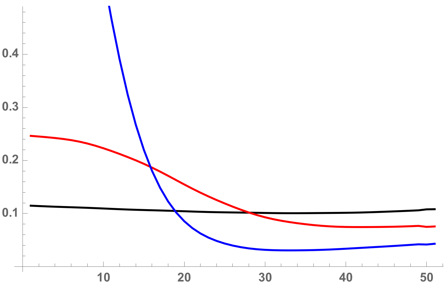
Then, we turned our attention to the problem of showing the existence of solutions to the eigenvalue problem for the family of transfer operators ${\mathcal{P}}_q^{\pm }$ of the Farey map with temperature q. In particular, we considered the problem of the existence of eigenfunctions with eigenvalue 1 and of a specific form as described in Theorem 3. A method to study this problem was introduced in [9,11,12] for the case of real values of q. It consists in rewriting the problem as a linear algebra problem for infinite matrices by looking for solutions in a specific Hilbert space of functions. This method was used in [9,10] to obtain properties of the spectrum of these operators. Unfortunately, if one wants to study the eigenvalue-1 problem for the operators ${\mathcal{P}}_q^{\pm }$ in connection with the spectral theory of the modular surface as outlined above, one needs to consider the case of complex temperature q. In the last part of the paper, we showed how to extend the matrix approach developed for real values of q to the case of $q\in \mathbb{C}$ with $\Re \left(q\right)>0$ (which is enough to obtain the spectrum of the Laplace–Beltrami operator on the modular surface and the zeroes of the Selberg Zeta function). In Theorems 4 and 5, we gave an explicit formulation for the linear algebra problems equivalent to the eigenvalue-1 problems for ${\mathcal{P}}_q^{\pm }$. The explicit formulations of the problem are useful for a numerical approach. By Theorem 3, the existence of a solution to problem (10) for a given value q implies that there exists a correspondent eigenvalue for the Laplace–Beltrami operator on the modular surface and in turn a zero of the Selberg Zeta function with real part $1/2$ (see, e.g., [18]). The spectrum of the Laplace–Beltrami operator and the position of the zeroes of the Selberg Zeta function have been largely studied also via numerical methods (see [20] and references therein); therefore, Theorem 4 represents a new approach to the problem. The expression of the Selberg Zeta function implies that problem (11) is instead related to the non-trivial zeroes of the Riemann Zeta function (see Theorem 3 (iii)). Therefore, Theorem 5 gives an equivalent formulation of the Riemann Hypothesis in terms of a linear problem for infinite matrices. One is thus interested to study which values of q problem (19) has a solution for. The numerical study of this problem is not trivial, as the functions involved in the computation of the vector ${\Psi }$ have oscillating behaviour for $q\in \mathbb{C}$ with a non-vanishing imaginary part. We present some preliminary results. Using the standard north-west corner approximation of the matrices $A_q^{+}$ and $D_q$, we computed the $N\times N$ matrices $A_q^{+}\left(N\right)$ and $D_q\left(N\right)$ and found the vector

$${\Phi }(N,q):={(A_q^{+}\left(N\right)-D_q\left(N\right))}^{-1}{D}_q\left(N\right){\Psi }\left(N\right)\in {\mathbb{C}}^N,$$

where ${\Psi }\left(N\right)={\left({{\Psi }}_n\right)}_{n=0,\cdots ,N-1}$. Then, we computed the norms

$${\parallel {\Phi }(N,q)\parallel }_2^2=\sum _{n=0}^{N-1}{\left|{\Phi }{(N,q)}_n\right|}^2\frac{\mathrm{\Gamma }(n+2\xi )}{n!}.$$

The Riemann Hypothesis is equivalent to the condition that ${\parallel {\Phi }(N,q)\parallel }_2$ remains finite as $N\to \infty$ only for values of q with $\xi =\Re \left(q\right)=1/4$ (recall that by Theorem 3 (iii) a solution to problem (19) exists for a given value q if and only if $2q$ is a zero of the Riemann Zeta function). In Figure 1, we plot the functions $q=(1/2+i\eta )/2\to {\parallel {\Phi }(N,q)\parallel }_2^2$ for $N=10,15,20$. The functions were obtained by using 50 values of $\eta$ uniformly distributed in the interval $(13.75,15.25)$, in order to include the first zero of the Riemann Zeta function on the critical line $\Re \left(2q\right)=1/2$ which has ${\eta }_0\approx 14.134725$ (corresponding to the value $\approx 12.8$ in the x-axis of the figure).

The figure suggests that for some values of q, including $1/2+i{\eta }_0$, the norms ${\parallel {\Phi }(N,q)\parallel }_2$ are not monotone with N, but are increasing for small values of N to be decreasing for larger values.

Finally, we add that it is possible to use the formulation in Theorem 5 by applying the results in [29]. In that paper, we proved in collaboration with S. Isola how to write as in (8) a one-parameter family of solutions ${\psi }_q^{+}$ to the problem ${\mathcal{P}}_q^{+}f=f$ which is well known to exist (see [17]). These functions are in one-to-one correspondence with the non-holomorphic Eisenstein series and give a direct way to check the validity of Theorem 3 (iii), since the term c in (8) for the functions ${\psi }_q^{+}$ is exactly the value of the Riemann Zeta function at $2q$ and the term b does not vanish for all q. It is then possible to use the expression (8) for the functions ${\psi }_q^{+}$ to find their expansion on the basis of the Laguerre polynomials and to find conditions for these functions to give solutions to problem (19). This approach is left for future work.

References

- Bowen, R. Equilibrium States and the Ergodic Theory of Anosov Diffeomorphisms, 2nd ed.; (with a preface by D., Ruelle); Chazottes, J.-R., Ed.; Lecture Notes in Mathematics, 470; Springer: Berlin/Heidelberg, Germany, 2008. [Google Scholar]
- Ruelle, D. Thermodynamic Formalism, 2nd ed.; Cambridge Mathematical Library; Cambridge University Press: Cambridge, UK, 2004. [Google Scholar]
- Bonanno, C.; Giulietti, P.; Lenci, M. Infinite mixing for one-dimensional maps with an indifferent fixed point. Nonlinearity 2018, 31, 5180–5213. [Google Scholar] [CrossRef] [Green Version]
- Melbourne, I.; Terhesiu, D. Operator renewal theory and mixing rates for dynamical systems with infinite measure. Invent. Math. 2012, 189, 61–110. [Google Scholar] [CrossRef] [Green Version]
- Gouëzel, S. Limit theorems in dynamical systems using the spectral method. In Hyperbolic Dynamics, Fluctuations and Large Deviations; Proceedings of Symposia in Pure Mathematics 89; American Mathematical Society: Providence, RI, USA, 2015; pp. 161–193. [Google Scholar]
- Keller, G. Equilibrium States in Ergodic Theory; London Mathematical Society Student Texts, 42; Cambridge University Press: Cambridge, UK, 1998. [Google Scholar]
- Prellberg, T. Towards a complete determination of the spectrum of a transfer operator associated with intermittency. J. Phys. A 2003, 36, 2455–2461. [Google Scholar] [CrossRef]
- Prellberg, T.; Slawny, J. Maps of intervals with indifferent fixed points: Thermodynamic formalism and phase transitions. J. Statist. Phys. 1992, 66, 503–514. [Google Scholar] [CrossRef] [Green Version]
- Ben Ammou, S.; Bonanno, C.; Chouari, I.; Isola, S. On the leading eigenvalue of transfer operators of the Farey map with real temperature. Chaos Solitons Fractals 2015, 71, 60–65. [Google Scholar] [CrossRef] [Green Version]
- Ben Ammou, S.; Bonanno, C.; Chouari, I.; Isola, S. On the spectrum of the transfer operators of a one-parameter family with intermittency transition. Far East J. Dyn. Syst. 2015, 27, 13–25. [Google Scholar] [CrossRef] [Green Version]
- Bonanno, C.; Graffi, S.; Isola, S. Spectral analysis of transfer operators associated to Farey fractions. Atti Accad. Naz. Lincei Rend. Lincei Mat. Appl. 2008, 19, 1–23. [Google Scholar] [CrossRef] [Green Version]
- Isola, S. On the spectrum of Farey and Gauss maps. Nonlinearity 2002, 15, 1521–1539. [Google Scholar] [CrossRef]
- Bruggeman, R.; Lewis, J.B.; Zagier, D. Function theory related to the group PSL2(R). In From Fourier Analysis and Number Theory to Radon Transforms and Geometry; Farkas, H.M., Gunnin, R.C., Knopp, M.I., Taylor, B.A., Eds.; Dev. Math., 28; Springer: New York, NY, USA, 2013; pp. 107–201.PSL2(R). [Google Scholar]
- Bruggeman, R.; Lewis, J.B.; Zagier, D. Period functions for Maass wave forms and cohomology. Mem. Amer. Math. Soc. 2015, 237, 1118. [Google Scholar] [CrossRef] [Green Version]
- Chang, C.-H.; Mayer, D.H. The period function of the nonholomorphic Eisenstein series for PSL(2,Z). Math. Phys. Electron. J. 1998, 4, 6. [Google Scholar]
- Lewis, J.B. Spaces of holomorphic functions equivalent to even Maass cusp forms. Invent. Math. 1997, 127, 271–306. [Google Scholar] [CrossRef]
- Lewis, J.B.; Zagier, D. Period functions for Maass wave forms. I. Ann. Math. 2001, 153, 191–258. [Google Scholar] [CrossRef]
- Mayer, D.H. The thermodynamic formalism approach to Selberg’s zeta function for PSL(2,Z). Bull. Amer. Math. Soc. 1991, 25, 55–60. [Google Scholar] [CrossRef] [Green Version]
- Pohl, A.; Zagier, D. Dynamics of geodesics and Maass cusp forms. Enseign. Math. 2020, 66, 305–340. [Google Scholar] [CrossRef]
- Fraczek, M.S. Selberg zeta Functions and Transfer Operators. An Experimental Approach to Singular Perturbations; Lecture Notes in Mathematics, 2139; Springer: Cham, Switzerland, 2017. [Google Scholar]
- Erdélyi, A.; Magnus, W.; Oberhettinger, F.; Tricomi, F.G. Higher Transcendental Functions. Vols. I, II’; Based, in part, on Notes Left by Harry Bateman; McGraw-Hill Book Co., Inc.: New York, NY, USA, 1953. [Google Scholar]
- Khinchin, A.Y. Continued Fractions; Translated from the Third (1961) Russian Edition; Reprint of the 1964 Translation; Dover Publications, Inc.: Mineola, NY, USA, 1997. [Google Scholar]
- Mayer, D.H. On the thermodynamic formalism for the Gauss map. Comm. Math. Phys. 1990, 130, 311–333. [Google Scholar] [CrossRef]
- Terras, A. Harmonic Analysis on Symmetric Spaces and Applications I; Springer: New York, NY, USA, 1985. [Google Scholar]
- Efrat, I. Dynamics of the continued fraction map and the spectral theory of SL(2,Z). Invent. Math. 1993, 114, 207–218. [Google Scholar] [CrossRef]
- Knauf, A. Number theory, dynamical systems and statistical mechanics. Rev. Math. Phys. 1999, 11, 1027–1060. [Google Scholar] [CrossRef] [Green Version]
- Iwaniec, H. Spectral Methods of Automorphic Forms, 2nd ed.; Graduate Studies in Mathematics, 53; American Mathematical Society: Providence, RI, USA; Revista Matemática Iberoamericana: Madrid, Spain, 2002. [Google Scholar]
- Bonanno, C.; Isola, S. A thermodynamic approach to two-variable Ruelle and Selberg zeta functions via the Farey map. Nonlinearity 2014, 27, 897–926. [Google Scholar] [CrossRef] [Green Version]
- Bonanno, C.; Isola, S. Series expansions for Maass forms on the full modular group from the Farey transfer operators. J. Number Theory 2020, 210, 183–230. [Google Scholar] [CrossRef] [Green Version]
- Ismail, M.E.H. Classical and Quantum Orthogonal Polynomials in One Variable; Encyclopedia of Mathematics and its Applications, 98; Cambridge University Press: Cambridge, UK, 2005. [Google Scholar]
- Srivastava, H.M.; Mavromatis, H.A.; Alassar, R.S. Remarks on some associated Laguerre integral results. Appl. Math. Lett. 2003, 16, 1131–1136. [Google Scholar] [CrossRef]
- Olver, F.W.J.; Lozier, D.W.; Boisvert, R.F.; Clark, C.W. (Eds.) NIST Handbook of Mathematical Functions; U.S. Department of Commerce, National Institute of Standards and Technology: Washington, DC, USA; Cambridge University Press: Cambridge, UK, 2010.
Figure 1.
The functions are plotted (the colours are: black for ; red for ; blue for ) in the interval . A value k in the x-axis corresponds to .
Disclaimer/Publisher’s Note: The statements, opinions and data contained in all publications are solely those of the individual author(s) and contributor(s) and not of MDPI and/or the editor(s). MDPI and/or the editor(s) disclaim responsibility for any injury to people or property resulting from any ideas, methods, instructions or products referred to in the content. |
© 2022 by the author. Licensee MDPI, Basel, Switzerland. This article is an open access article distributed under the terms and conditions of the Creative Commons Attribution (CC BY) license (https://creativecommons.org/licenses/by/4.0/).
Share and Cite
MDPI and ACS Style
Bonanno, C. On the Generalised Transfer Operators of the Farey Map with Complex Temperature. Mathematics 2023, 11, 134. https://doi.org/10.3390/math11010134
AMA Style
Bonanno C. On the Generalised Transfer Operators of the Farey Map with Complex Temperature. Mathematics. 2023; 11(1):134. https://doi.org/10.3390/math11010134
Chicago/Turabian StyleBonanno, Claudio. 2023. "On the Generalised Transfer Operators of the Farey Map with Complex Temperature" Mathematics 11, no. 1: 134. https://doi.org/10.3390/math11010134
Note that from the first issue of 2016, this journal uses article numbers instead of page numbers. See further details here.