Abstract
Data at a smaller regional level has now become a necessity for local governments. The average data on household expenditure on food and non-food is designed for provincial and district/city estimation levels. Subdistrict-level statistics are not currently available. Small area estimation (SAE) is one method to address the problem. The Empirical Best Linear Unbiased Prediction (EBLUP)—Fay Herriot Multivariate method estimates the average household expenditure on food and non-food at the sub-district level in Central Java Province in 2020. Meanwhile, for the sub-districts that are not sampled, the estimation of average household expenditure is done by adding cluster information to the EBLUP Multivariate modeling. The K-Medoids Cluster method is used to classify sub-districts based on their characteristics. Small area estimation using the EBLUP-FH Multivariate method can enhance the parameter estimations obtained using the direct estimation method because it results in a lower level of variation (RSE). For sub-districts that are not sampled, the Residual Standard Error (RSE) value from the estimated results using the EBLUP-FH Multivariate method with cluster information is lower than 25%, indicating that the estimate is accurate.
MSC:
62F10
1. Introduction
Unquestionably, the current era of economic disruption has a negative side that is particularly felt by middle- to low-income individuals. Disruptions to the economy can eliminate the economic growth momentum generated by demographic bonuses. Numerous jobs previously performed by humans are being replaced by technological innovation and various forms of artificial intelligence. It will lead to new inequality issues as a result of labour reduction, ultimately affecting the welfare of the community. In order to prevent economic disruption from aggravating existing welfare issues in Indonesia, particularly for vulnerable communities and households, the government must implement optimal policies.
The welfare of the population in an area can be described through several indicators, one of which is household consumption expenditure (Sekhampu and Niyimbanira [1]; Irawan, et al. [2]). The presentation of household consumption expenditure data produced by the Central Bureau of Statistics (BPS) via the National Socio-Economic Survey (Susenas) must be expanded in order to estimate population parameters at the national, provincial, and district/city levels. It is not designed to estimate population parameters in smaller areas, such as sub-districts or villages, because the sample size is insufficient. The government now requires data presented at a more detailed and accurate regional level in order to conduct development planning and evaluation as well as address population welfare and inequality issues in a targeted and effective manner. Due to a lack of information at the subregional level, policymaking and implementation by local governments are less optimized.
In addition, the sustainable development goals (SDGs) targeted by the United Nations (UN) must be provided by each member country, including Indonesia. Obviously, the fulfillment of the SDGs target requires an estimation level at smaller geographical areas such as districts/cities, sub-districts, and even at the village level. However, the limited number of samples in surveys conducted by BPS will result in inadequate precision for estimation values or parameter estimation in small areas due to the large variance of the resulting estimates. The provision of more budget to increase the number of samples and the number of survey officers is one effort that can be made so that the existing survey design is able to provide a direct estimation of statistical output in small areas with adequate precision, one of which is for the estimation of average household expenditure.
This data is one of the key components required in calculating the poverty rate of a region. The estimation of average household expenditure data up to the sub-district level can later be used as an indicator in grouping sub-districts in a region based on expenditure groups. In addition, the estimated data can be used as an indicator to rank regions to obtain regions that will be the target of poverty alleviation programs or community welfare improvement programs by the regional government. The importance of the need for information down to the small-area level and the limitations of existing resources make it necessary for BPS to apply a statistical method capable of handling these problems. According to Notodiputro and Kurnia [3], one possible solution is the indirect estimator, known as small area estimation (SAE).
Rao and Molina [4] explained that the application of SAE is conducted by borrowing strength from the information of auxiliary variables associated with the response variable or the estimated variable. This condition allows SAE to be employed to improve the effectiveness of survey sample collection at BPS. Several estimation methods can be conducted in SAE, including Best Linear Unbiased Prediction (BLUP), Empirical Best Linear Unbiased Prediction (EBLUP), Hierarchical Bayes (HB), and Empirical Bayes (EB). In general, the selection criteria for these estimation methods are determined based on the type of data on the response variable. EB and HB methods are generally used on response variables that are binary or enumerated, while BLUP and EBLUP methods are more appropriate for continuous response variables (Rao and Molina [4]). The EBLUP method is a form of General Linear Mix Model (GLMM) when the parameter variance is unknown and is considered to have several advantages over other models (Ghosh and Rao [5]). Fay and Herriot [6] initiated using the EBLUP estimation method in area-level SAE to estimate the logarithm of the per capita income of the United States population. Therefore, this model is known as the Fay–Herriot model.
Many research variables, including variables generated from BPS surveys, have strong correlations. One example is the correlation between average household food expenditure and average household non-food expenditure (Nurizza [7]). These strongly correlated variables can be estimated together using the Multivariate EBLUP SAE method and are expected to have a more efficient estimation value than Univariate EBLUP SAE (Datta, Fay, and Ghosh, [8]). The Multivariate Fay–Herriot or Multivariate EBLUP model was then developed by Benavent and Morales [9] by presenting four different estimation models based on the structure of the covariance matrix.
Based on the condition of the March 2020 National Socio-Economic Survey (Susenas) data for Central Java Province, out of a total of 576 sub-districts, 573 sub-districts were included as samples. There were three sub-districts that were not selected as Susenas samples (BPS [10]). Because not all sub-districts were selected as Susenas samples, the problem is how to estimate the parameters for unsampled sub-districts. In estimating EBLUP for unsampled areas, a global synthetic model is usually used. Rao [11] stated that a synthetic estimator is an unbiased estimator in a large area that is used to obtain an indirect estimator in a small area, assuming that the small area has the same characteristics as the large area. The synthetic estimator model will ignore the random area effect since the random area effect information does not exist in the unsampled area (Saei and Chambers [12]), so that the estimation in unsampled subdistricts may be biased.
Some studies with the EBLUP method utilize the addition of cluster information in estimating unsampled areas. Ginanjar [13] researched some of them, who estimated per capita expenditure at the sub-district level in Jambi Province in unsampled sub-districts using the univariate EBLUP method with the addition of cluster information. With the same method, Anisa et al. [14] also added the mean value of the random area effect estimator in each cluster to the prediction model to estimate the unsampled area. Meanwhile, with the Fay–Herriot Multivariate model, Nuryadin [15] applied cluster information to predict the average per capita expenditure per village for food and non-food in unsampled villages. These studies conclude that models that are first clustered turn out to provide better predictions than models without clustering. There has been no research on the EBLUP-FH Multivariate method with K-Medoids Cluster information for actual data compared with the direct estimation method.
The clustering technique commonly used by researchers is K-Means Cluster. However, K-Means Cluster is highly sensitive to large data containing outliers, so the K-Medoids Cluster technique is a better alternative in this condition because it is more robust to outliers (Patel and Singh [16]; Sangga [17]). Based on this explanation, this study compares the direct estimation method and the EBLUP-FH Multivariate method in estimating the average household expenditure on food and non-food at the sub-district level in Central Java Province. In addition, this research also estimates the average household expenditure on food and non-food in non-sampled areas (sub-districts) using the EBLUP-FH Multivariate method by applying K-Medoids Cluster information. The K-Medoids cluster technique is based on considering a large amount of data and the presence of outliers in the auxiliary variables used.
2. Materials and Methods
Table 1 below presents a summary of the materials and methods used in this research. The detailed explanation will be presented in the following subsections.

Table 1.
Summary of Research Materials and Methods.
2.1. Average of Household Expenditures
BPS [10] defines average household expenditure as the monthly costs incurred for all household members’ consumption, divided by the number of households. Household consumption can be divided into food and non-food consumption and is restricted to spending on household necessities only, without consideration of sources. The forms of consumption expenditures include purchases, gifts, and items generated by the household (excluding expenditures used for business purposes or those given to other parties).
The calculation of average household expenditure in the i-th area can be mathematically formulated as follows:
where:
- : average monthly household expenditure in the i-th area (rupiah)
- : total household expenditure in a month in the i-th area (rupiah)
- : number of households
2.2. Related Research on Determining Auxiliary Variables
Rao [18] states that in conducting indirect estimation, the choice of auxiliary variables is very significant in determining the accuracy of the resulting estimates. Estimation of per capita expenditure variables using small area estimation, or SAE, has been done quite a lot in Indonesia. Desiyanti et al. [19] use the EBLUP Univariate method to estimate average per capita expenditure at the sub-district level in West Sumatra. However, estimation of unsampled sub-districts still uses synthetic estimators. Auxiliary variables used in indirect estimation are the number of non-electricity user families, the number of non-PLN electricity user families, the number of polyclinics/medical centers, the number of minimarkets/supermarkets, the number of SD/MI, and the number of doctor’s practices.
In Amaliana and Lestari’s research [20] on the application of the EBLUP Univariate method to the Fay–Herriot SAE model, the auxiliary variables used including the percentage of agricultural households, the number of Insurance for the Indigence recipients, State Electricity Company (PLN) electricity users, the number of Elementary School (SD)-Junior High School (SMP)-High School (SMA)- University (PT), the number of families living in slums, the number of Certificate of Indigence (SKTM) owners, the number of educational institutions and skills, and the number of Indonesian migrant workers (TKI) have a significant effect in indirectly estimating per capita expenditure in the Jember District.
Furthermore, Nurizza and Ubaidillah [21] used the SAE multivariate approach in estimating food and non-food per capita expenditure in Indonesia. Their results shows that in estimating indirect per capita food expenditure, the variables of the number of non-PLN electricity users, the number of riverbank settlements, the number of migrant workers, elementary schools, vocational schools, universities, auxiliary health centers, polyclinics, doctor’s offices, village maternity clinics, integrated health posts, medium and small industries (IMK), restaurants and inns had a significant effect. Meanwhile, for the indirect estimation of non-food per capita expenditure in Indonesia, the variables that have a significant effect are the number of PLN electricity users, non-PLN users, migrant workers, elementary schools, midwife practice sites, doctor practice sites, village maternity clinics, integrated health posts, community health centers without inpatient care, auxiliary community health centers, polyclinics, pharmacies, and restaurants.
Small-area estimation of per capita expenditure at the subdistrict level was also conducted by Ginanjar [13] using the EBLUP method in Jambi Province. In this study, there were eight auxiliary variables or predictor variables that significantly influenced per capita expenditure at the subdistrict level in Jambi Province, namely population, number of universities, the ratio of school facilities, number of polyclinics/health centers, coverage of doctors, coverage of health workers, coverage of people with disabilities, and the ratio of midwives.
2.3. Small Area Estimation
An area is considered large if the sample drawn from it is large enough to yield a direct estimate with sufficient precision. Conversely, an area or domain is considered small if the domain-specific sample is not large enough to support direct estimation with sufficient precision or accuracy (Rao and Molina [4]). Small area estimation (SAE) is an indirect estimation technique in small areas that is conducted by borrowing strengths from related areas and/or periods to increase the effectiveness of the sample size and decrease the standard error, allowing the estimation results to have sufficient precision (Rao and Molina [4]).
The main problems in SAE are how to produce reasonably good parameter estimates in an area with a relatively small sample size and how to estimate the mean square error (MSE) of the resulting parameter estimates (Pfeffermann [22]). Both of these main points can be generated by borrowing additional information from within the area, outside the area, or outside the survey (auxiliary variables), which can usually be obtained from census or administrative data.
Based on the availability of auxiliary variables, SAE can be classified into two types (Rao dan Molina [4]).
2.3.1. Basic Unit-Level Model
The unit-based small area estimation model is an SAE model with available auxiliary variables corresponding to response variables observed up to the unit level. Assumed auxiliary variables are available for every j-th element in the i-th area. available for each j-th element in the i-th area. The variables of interest are assumed to have a relationship with through the following equation:
Area random effects are denoted by , a random variable that is assumed to be independent and identically distributed. While for with a known constant and are random variables that are mutually independent and identically distributed with respect to . In other words, and are generally assumed to have a normal probability distribution.
2.3.2. Area-Level Model (Basic Area-Level)
The area-based SAE model introduced by Fay and Herriot in 1979 is part of the General Linear Mixed Model (GLMM). This GLMM model is built based on the availability of predictor variables and direct estimation at a certain area level. Suppose there are a number of small areas as many as ( with auxiliary variable data available for each i-th small area being , with the parameters to be estimated being . The is assumed to be linearly related to through the following equation (Ubaidillah [23]):
By:
- is a vector of regression coefficients of size p × 1
- : known positive constant
- : small area random effects, with assumed to be independent and identically distributed (iid) with and .
If assumed is an unbiased direct estimator for , where the estimator contains the error of the sample draw, namely , then the sampling model can be formulated as follows:
where is a sampling error that is assumed to be independent of each other with its variance assumed to be known () or and .
Combining Equations (1) and (2) will result in a General Linear Mixed Model of area-based small area estimation known as the Fay–Herriot model, namely:
In the model Equation (3) above, the variation of the response variable in a small area is assumed to be explained by the relationship between the response variable and the auxiliary variables, which is called the fixed effect model. In addition, this model also contains a small area random effect component, which is a small area-specific variation component that cannot be explained by the auxiliary variables. The combination of these two assumptions (the fixed effect model and the random effect model) forms a linear mixed model.
2.4. Multivariate Fay–Herriot Models
The Multivariate Fay–Herriot model is a development of the Univariate Fay–Herriot model that can be used for more than one response variable (Ubaidillah [23]). Suppose the population is partitioned into area. Let be a vector of the -th variable of interest, with . Meanwhile, the vector of -th direct estimators of is denoted by . As for , it is assumed to be related to area-specific auxiliary variables through a linear model (Ubaidillah, 2017):
where:
- : vector of area random effects
- : covariance matrix of area random effects of size
- : -th matrix of area-specific auxiliary variables of size with
- : vector of regression coefficients, with
The sampling model can be formulated as follows:
where is the vector of sampling errors and is a known covariance matrix of size . By combining Equations (4) and (5), the Multivariate Fay–Herriot model is generated as follows:
where and are independent.
The model in Equation (6) can be written in matrix form as follows (Benavent and Morales, 2016):
where and are mutually independent. is a matrix of random effect constants that are assumed to be known. The matrix with is a matrix of auxiliary variables with . The vector is the vector of variables of interest with . The operator means stacking matrix by column. The matrix is the covariance matrix of the random effects area where is the identity matrix of size , and denotes a Kronecker product. While is a sampling covariance matrix of size which is assumed to be known and obtained from sampling error in the survey.
Empirical Best Linear Unbiased Prediction (EBLUP) Multivariate
Under the model in Equation (7), it holds that and . The best linear unbiased prediction (BLUP) of where is:
where is the best linear unbiased estimator (BLUE) of .
Since the value of the random effect variance component, is unknown, it must be determined from empirical data when modeling parameters using the EBLUP-Fay–Herriot approach. There are several estimation methods that can be performed on the random effect variance component, such as the Maximum Likelihood (ML) and Restricted Maximum Likelihood (REML) methods based on normal likelihood (Patterson and Thompson [24]).
As stated earlier, the multivariate BLUP estimator (8) depends on the variance parameter of where . The variance parameter,, cannot be known and is estimated using the REML approach. Restricted log-likelihood of the joint probability density of which is expressed as a function of is given as follows (Benavent and Morales [9]):
where . By taking the partial derivative of Equation (9) with respect to with -th element, where , then the score vector is obtained where:
where is the partial derivative of with respect to -th element of . By taking the second order partial derivative of Equation (9) with respect to with -th element, changing sign and taking expectations, then the Fisher Information matrix is obtained as follows:
The iterative of Fisher-scoring algorithm for REML estimation of is:
Furthermore, the Empirical Best Linear Unbiased Prediction (EBLUP) estimator for the Multivariate Fay–Herriot model is obtained by plugging in and of Equation (8) as follows:
where is the Best Linear Unbiased Estimator (BLUE) for with covariance matrix .
2.5. Direct Estimation
Estimation of population parameters in a region based only on sample data from that region is said to be direct estimation (Rao and Molina [4]). This direct estimation method is design-based or depends on the sampling design used. The March 2020 National Socio-Economic Survey (Susenas) results were used in this study to directly estimate the response variable on average household expenditure on food and non-food.
2.6. Selection of Auxiliary Variables
The auxiliary variables used in SAE must be related to the response variable. The auxiliary variables used in this study were taken from the variables used in related studies and then grouped into variable groups with the following details:
- Population
- Education
- Health
- Economy (industry)
- Economy (other than industry)
- Economy (financial inclusiveness)
There are methods we can use to select auxiliary variables, including forward, backward, and stepwise methods. The stepwise selection method combines the forward and backward selection methods. The stepwise method modifies the forward selection method. When a new variable is added, all candidate variables in the model are checked again to see if they are still significant. If there is a variable that becomes insignificant based on the specified significance level, then the variable is removed (backward). In this stepwise method, there are two levels of significance: adding variables and removing variables from the model.
2.7. Multivariate EBLUP Method with Added Cluster Information
The EBLUP method is generally used to estimate an area that contains a sample. Unsampled areas can usually be estimated using a synthetic model. The problem with the synthetic model is that it does not consider the random effect area because it does not have enough information about the area that was not sampled. It can lead to an estimated value with a large bias (. Therefore, adding cluster information to the EBLUP method should improve estimates for unsampled areas. Clustering is conducted based on auxiliary variables so that all areas will be included in certain clusters, both with and without samples.
The addition of cluster information is based on the assumption that an area has a pattern of close relationships with other areas. The random area effect has a similarity pattern between areas, allowing it to be analyzed using cluster techniques from the auxiliary variables in each small area. In estimating an unsampled area, the random area effect is often ignored due to the absence of such information. The EBLUP estimator for unsampled areas can be modeled as follows:
with are the unsampled subdistricts in this study (Padureso sub-district, Batuwarno sub-district, and Lebakbarang sub-district).
The sampled and unsampled sub-districts will be grouped based on the auxiliary variables so that the cluster for each sub-district can be identified. The auxiliary variables used are selected variables that have met the assumptions of sample adequacy and non-multicollinearity first. The next step to be done in the sampled sub-districts is to average the random area effects per known cluster. Then the average of the random area effect per cluster will be entered into the prediction model as the estimator of the random area effect. The average random area effect per cluster is formulated in the following equation:
with
- : number of sub-districts sampled in the -th cluster
- : the average random effect area in the -th cluster
- : random effect area in the -th sample
The average random effect area is used as additional information in areas where there are no samples in the corresponding cluster. Thus, the EBLUP estimator for unsampled areas can be formulated as follows:
with are the unsampled subdistricts in the -th cluster and is the average of random effect area in the -th cluster.
The quality of the resulting estimates can be evaluated based on the Relative Standard Error (RSE) value. The RSE value for the Multivariate EBLUP method is obtained by comparing the square root value of the MSE to the estimated value of the response variable, expressed as a percentage, according to the following formula:
According to BPS (2020), decisions regarding the accuracy of an estimate with RSE conditions 25% the resulting data is accurate (and can be used), condition 25% RSE 50% needs to be careful if the data will be used, and the condition RSE % data is considered inaccurate. The greater the RSE value, the more the estimator value differs significantly from the real parameter value.
2.8. Research Stages
The stages of research using the Multivariate EBLUP method and with the addition of cluster information are as follows:
- 1.
- Prepare response variable data from National Socio-Economic Survey (Susenas) March 2020 data and auxiliary variable data from Village Potential Podes 2020 data for each sub-district in Central Java Province.
- 2.
- Prepare the direct estimation results for the response variable of average household food and non-food expenditures that have been obtained from the results of the March 2020 National Socio-Economic Survey (Susenas) processing, namely 573 sub-districts out of a total of 576 sub-districts in Central Java Province.
- 3.
- Test the correlation between the response variables average household expenditure on food and average household expenditure on non-food with Pearson Correlation.
The Pearson Correlation test hypothesis is as follows:
with the Pearson correlation coefficient formula as follows:
To test the significance of the correlation, the t-test is used with the following formula:
where:
- m = sample size
- r = the computed correlation coefficient being tested for significance.
The t-distribution formula for obtaining the appropriate t-value for testing the significance of the correlation coefficient is given by Equation (16). Then, the results of Equation (16) are compared to the t-table values with degrees of freedom . If , then will be rejected or if the p-value is less than which is set at 0.05.
- 4.
- In the sampled area, the SAE area-level model was built to estimate parameters through the Multivariate EBLUP method, namely by:
- a.
- Estimating the variance component using the REML method through the Fisher scoring iteration procedure, according to Equation (10). The estimation process was conducted with the help of open-source R software version 4.1.3, using the package "msaeDB".
- b.
- Estimating where
- c.
- Perform the selection of auxiliary variables using the stepwise method
- d.
- Estimating the average household expenditure on food and non-food () in each sampled sub-district using the selected auxiliary variables according to Equation (11)
- e.
- Calculate the RSE values of EBLUP-FH Multivariate on the average of household expenditure on food and non-food for each sub-district according to Equation (14)
- 5.
- Perform the estimation process on non-sampled sub-districts using the Multivariate EBLUP method by adding cluster information with the K-Medoids technique, preceded by the following steps:
- a.
- Checking the assumption of sample adequacy (KMO value) and detecting multicollinearity.
- b.
- Apply the Z-Score approach to standardize the auxiliary variables used in the clustering procedure.
- c.
- Determination of the optimum number of clusters using the silhouette method.
- d.
- In the sampled area, the known components are averaged in each cluster according to equation (12).
- e.
- Estimating the average household expenditure on food and non-food in the non-sampled area using the EBLUP-FH Multivariate method by adding cluster information ( according to equation (13). The estimation process uses R software with the “msaeDB” package and “msaefhns” function.
- 6.
- Analyzing the results of estimating the average household expenditure on food and non-food at the sub-district level in Central Java Province.
2.9. Data Source
This research uses secondary data from the Central Bureau of Statistics (BPS) as follows:
- 1.
- Average monthly household expenditure on food and non-food data for 573 sub-districts in Central Java Province, sourced from the March 2020 National Socio-Economic Survey (Susenas) raw data using the direct estimation method. This data is used as response variables.
- 2.
- Data on facilities, infrastructure, and other auxiliary variables available in each sub-district in Central Java Province were sourced from processing Village Potential (Podes) 2020 raw data.
This research is a case study for all sub-districts (576 sub-districts) in the districts/cities of Central Java Province in 2020. The National Socio-Economic Survey (Susenas) and Podes data used are aggregated data for each sub-district in Central Java Province. The processing in this study was carried out using the open-source software R version 4.1.3.
2.10. Research Variables
The variables used in this study include response variables and auxiliary variables. The response variable used is the average monthly food and non-food consumption expenditure of households in the i-th sub-districts, sourced from the March 2020 National Socio-Economic Survey (SUSENAS) data. Meanwhile, auxiliary variables in each sub-district are obtained from PODES data in the 2020 Central Java Province. The determination of the auxiliary variables in this study is based on factors that affect the average household food and non-food consumption expenditure. The 40 candidates for auxiliary variables are shown in Appendix A, Table A1. Meanwhile, the significant auxiliary variables included in the model are presented in Table 2.
Table 2.
Selected Significant Auxiliary Variables.
3. Results
In Section 3, the study’s results are introduced along with a general overview of welfare problems in Central Java Province, Indonesia. For both the sub-districts sampled for the March 2020 Susenas and those not sampled, the findings from the estimation of the average household expenditure on food and non-food items will be provided. Maps of distribution, graphs, and boxplots of RSE values will be used to compare the results between the direct estimation and the EBLUP-FH Multivariate method for the 573 sampled sub-districts. In addition, the EBLUP-FH Multivariate method’s findings for the estimation of non-sampled sub-districts are shown in this section.
3.1. Overview of Central Java Province
In 2020, Central Java had an economic share of 8.55 percent (Figure 1), which was the fourth largest contributor to the national economy, after DKI Jakarta (17.55 percent), East Java (14.58 percent), and West Java (13.22 percent). However, all levels of society did not equally enjoy a high share of Central Java’s economy. It was reflected in the percentage of poverty which ranked as the second highest in Java after Yogyakarta, or ranked 13th nationally, with a poverty, percentage of 11.41 percent.
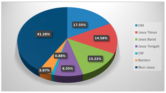
Figure 1.
Share of the economy in Indonesia in 2020. Source: Central Bureau of Statistics.
When the poverty rate is broken down by district/city, 23 out of 29 districts in Central Java have a poverty rate above the national rate (Figure 2). Meanwhile, the poverty rates in the six cities in Central Java are far below the national rate. The calculation of poverty cannot be separated from the indicator of average household expenditure on both food and non-food items.
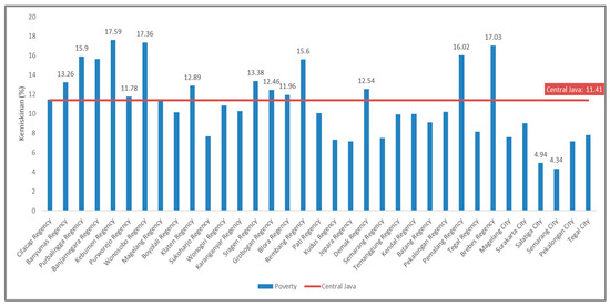
Figure 2.
Poverty Percentage in Central Java Province by District/City in 2020. Source: Central Bureau of Statistics.
3.2. Direct Estimation
The March 2020 National Socio-Economic Survey sampling design was used to get the direct estimates for the average household expenditure on food and non-food items. According to the sampling plan in Appendix B Table A2, parameters are estimated at the district or city level using a two-stage, one-phase sampling method. Direct estimation of average household expenditure on food and non-food can only be conducted in areas sampled in the March 2020 National Socio-Economic Survey (Susenas). In total, Central Java has 576 sub-districts. Out of these sub-districts, only 573 sub-districts were sampled in the March 2020 National Socio-Economic Survey (Susenas). The results of the direct estimation calculation were not obtained for the Padureso sub-district in the Kebumen district, the Batuwarno sub-district in the Wonogiri district, and the Lebakbarang sub-district in the Pekalongan district because these three sub-districts were not sampled in the March 2020 National Socio-Economic Survey (Susenas).
Using the direct estimation method to estimate the average household expenditure on food at the subdistrict level, the difference in expenditure figures between sub-districts is significant. Figure 3 shows the map of the estimated results for the average household expenditure on food per sub-district based on the direct estimation method. Wonogiri District’s Paranggupito Subdistrict has the lowest average household food expenditure of IDR 796,888. The sub-district of Banyumanik in the city of Semarang has the highest average household expenditures on food, at IDR 3,324,899. The median of average household food expenditure is IDR 1,668,801, indicating that 50 percent of sub-districts have average household food expenditures that are less than or equal to IDR 1,668,801.
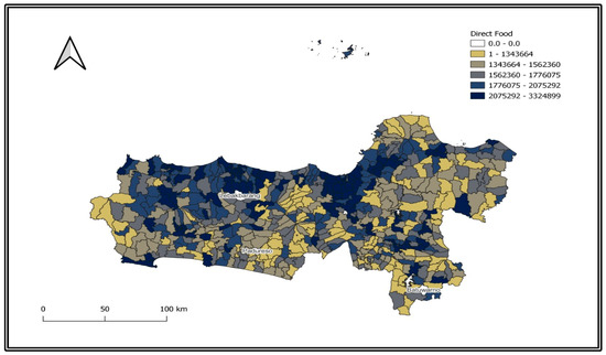
Figure 3.
Map of Estimation of Average Household Expenditure on Food at the Subdistrict Level in Central Java Province using the Direct Estimation Method.
The average household expenditure on non-food items varies greatly across subdistricts, according to direct estimates (Figure 4). Geyer sub-district in Grobogan District has the lowest average household expenditure on non-food items at IDR 486,601. In line with food expenditure, the sub-district of Banyumanik in Semarang City has the highest average value of non-food household expenditure at IDR 7,680,844.
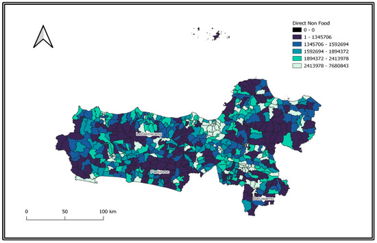
Figure 4.
Map of Estimation of Average Household Expenditure on Non-Food at the Subdistrict Level in Central Java Province using the Direct Estimation Method.
3.3. Multivariate Empirical Best Linear Unbiased Prediction (EBLUP) Modeling
3.3.1. Correlation Test of Response Variables
According to the results of the Pearson Correlation test in Equations (15) and (16), the p-value is less than 0.05, indicating that there is a correlation between the two response variables employed in the study. The correlation coefficient between the two response variables is 0.6216, which falls within the strong correlation range (De Vaus [25]). Therefore, the Multivariate Fay–Herriot EBLUP model can be applied to the variable that represents the average household expenditures for food and non-food in 2020 in Central Java.
3.3.2. Selection of Auxiliary Variables
After obtaining the results of the direct estimation of household expenditure at the sub-district level, estimation is carried out using the EBLUP-FH method. However, before estimating EBLUP-FH, the selection of auxiliary variables is first carried out based on the correlation value and its significance to the direct estimation. The selection of auxiliary variables was carried out using the stepwise method with a significance level of five percent. From the initial 40 candidate auxiliary variables, 13 significant auxiliary variables were generated for Multivariate EBLUP modeling of average household expenditure data for food (, the number of families using electricity (, number of elementary/islamic elementary school (, number of junior high school / Islamic junior high school (, number of polyclinics/medical centers (, number of doctor’s offices (, number of midwife practice sites (, number of village health posts (, number of small medium industry (IMK) from fabric/weaving (, total IMK of food and beverages (, number of other of small medium industry (, number of markets with permanent buildings (, number of markets with semi-permanent buildings (, and number of inns (.
Meanwhile, for Multivariate EBLUP modeling of average household expenditure data for non-food (, eight significant auxiliary variables were generated, namely the number of families using electricity (, the number of junior high schools/Islamic junior high schools (, number of universities/colleges (, number of polyclinics/medical centers (, number of doctor’s offices (, number of markets with permanent buildings (, number of minimarkets/supermarkets (, and number of restaurants/eateries (.
3.3.3. Fay–Herriot EBLUP Estimation for the Sampled Area
The results of estimating the regression coefficients of 13 auxiliary variables and 8 selected auxiliary variables can be seen in Table 3 and Table 4. The results of the modeling of the average household expenditure data for food and non-food in Table 3 and Table 4 are then used to estimate the small area of the average household expenditure variables for food and non-food in all sampled sub-districts of the National Socio-Economic Survey (Susenas) in March 2020.
Table 3.
Modeling Results of Average Household Expenditure on Food Data Using Multivariate EBLUP.
Table 4.
Modeling Results of Average Household Expenditure on Non-Food Using Multivariate EBLUP.
Figure 5 and Figure 6 below show a comparison of the results of direct estimation and the results of Multivariate EBLUP estimation for each variable of average household expenditure on food and non-food. Figure 5 and Figure 6 show that the results of estimating the average household expenditure on food and non-food using the Multivariate EBLUP method tend to be lower than the results of the direct estimate for the 573 sampled sub-districts.
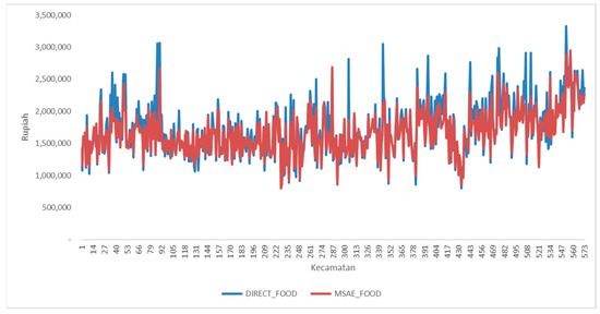
Figure 5.
Estimation of Average Household Expenditure on Food at the Subdistrict Level in Central Java Province Using the Direct Estimation Method and the Multivariate EBLUP Method.
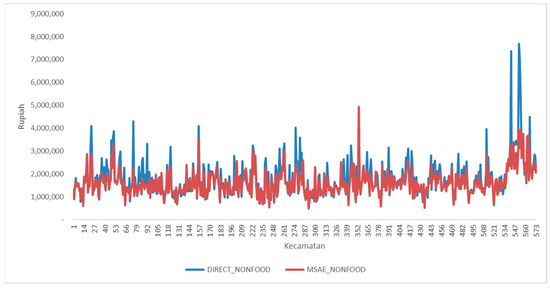
Figure 6.
Estimation of Average Household Expenditure on Non-Food at the Subdistrict Level in Central Java Province Using the Direct Estimation Method and the Multivariate EBLUP Method.
After estimating the regression coefficients, the RSE values of the direct and indirect estimate results (EBLUP-FH Multivariate) were compared. Figure 7 and Figure 8 show the RSE values of the direct estimator and the EBLUP-FH Multivariate estimate for average household expenditure on food and non-food in the sampled sub-districts of Central Java.
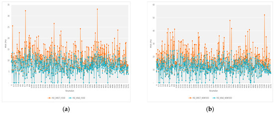
Figure 7.
RSE (%) of Direct Estimation and Multivariate EBLUP Model for Average Household Expenditure Variables at Subdistrict Level in Central Java: (a) for food; (b) for non-food.
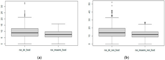
Figure 8.
Boxplot of RSE (%) of Direct Estimation and Multivariate EBLUP Model for Average District Level Household Expenditure Variables in Central Java: (a) for food; (b) for non-food.
Figure 7 demonstrates that the Multivariate EBLUP model provides a lower RSE value for the average household expenditure variable for food and non-food than the direct estimation. The RSE value of the Multivariate EBLUP model is less than 25 percent in all Central Java sub-districts.
Based on the boxplot in Figure 8, we can see that the results of the direct estimation of the average household expenditure variable for food and non-food at the sub-district level have a wider RSE range than the Multivariate EBLUP method. Although there are still outliers in the RSE value of the direct estimation and the Multivariate EBLUP model on the average household expenditure variable for non-food, the outliers in the Multivariate EBLUP model are significantly fewer in number and close to the tail of the boxplot. It can be concluded that the Multivariate EBLUP method produces a smaller level of diversity than the direct estimation method.
3.3.4. Estimation of Non-Sampled Subdistricts
The estimation of average household expenditure on food and non-food in non-sampled sub-districts of the National Socio-Economic Survey (Susenas) March 2020, was carried out by utilizing non-hierarchical clustering information using the K-Medoids cluster technique. This clustering process uses selected auxiliary variables for each response variable so that later clusters will be formed for modeling average household expenditure on food and clusters for modeling average household expenditure on non-food. Before further analysis is carried out using the K-Medoids cluster method, standardization is first carried out using the Z-Score method for each auxiliary variable used in clustering.
The next step is to check the assumption of sample adequacy by calculating the Kaiser-Meyer-Olkin (KMO) value. The processing results produced a KMO value of 0.72 and 0.82 for each auxiliary variable used in modeling average household expenditure on food and non-food, respectively. It can be concluded that the number of samples is sufficient or has adequately represented the population, allowing for further analysis.
Detection of multicollinearity is also carried out on auxiliary variables using the Variance Inflation Factor (VIF) value. The VIF values of thirteen auxiliary variables for the average household expenditure on food () and eight auxiliary variables for the average household expenditure on non-food () are shown in Table 5 and Table 6 below.
Table 5.
VIF Values of Thirteen Auxiliary Variables for Average Household Expenditure on Food.
Table 6.
VIF Values of the Eight Auxiliary Variables for Average Household Expenditure on Non-Food.
Based on the results in Table 5 and Table 6, the VIF value of the selected auxiliary variables for each average household expenditure response variable is less than 10. This means that there is no multicollinearity between the auxiliary variables. After the two cluster assumptions are met, the two groups of auxiliary variables will be used in cluster formation using the K-Medoids Cluster technique. The clustering process was carried out on all 576 sub-districts in Central Java for each group of auxiliary variables. The determination of the number of clusters in K-Medoids is based on the average silhouette method shown in Figure 9.
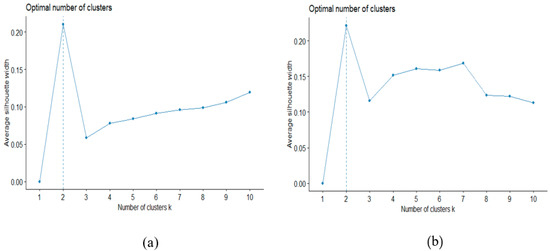
Figure 9.
Determination of the Optimal Number of Clusters by the Average Silhouette Method (a) Optimal number of Clusters for Average Food Expenditure (b) Optimal number of Clusters for Average Non-Food Expenditure.
Based on Figure 9, it can be seen that the highest average silhouette value is in the number of clusters of two clusters, both for the average food and non-food expenditure. As a result, this study will employ up to two clusters in grouping sub-districts using the K-Medoids Cluster method. In the average household expenditure group for food, cluster 1 consists of 380 sub-districts, and cluster 2 consists of 196 sub-districts. Meanwhile, cluster 1 in the non-food average household expenditure group consists of 260 sub-districts, and cluster 2 consists of 316 sub-districts. The characteristics of cluster 2 are generally those sub-districts with greater education and health infrastructure than cluster 1.
After the sub-district clusters are formed, the next step is to use the known components of random area effects per cluster and then average them per cluster. Then the average of the random area effects per cluster will be entered into the Multivariate EBLUP model as an estimator of the random area effects of the non-sampled sub-districts in the March 2020 National Socio-Economic Survey (Susenas). Estimates of average household expenditure on food and non-food in unsampled sub-districts resulting from Multivariate EBLUP modeling with the addition of cluster information are shown in Table 7 and Table 8.
Table 7.
Average household expenditure on food in non-sampled sub-districts.
Table 8.
Average household Expenditure on non-food in non-sampled sub-districts.
3.4. Mapping of Estimates of Average Subdistrict Level Household Expenditure from Multivariate EBLUP Modeling Results
The mapping of the estimation of the average household expenditure per sub-district is conducted based on the results of the estimation of the average sub-district level household expenditure obtained from the Multivariate EBLUP modeling with the addition of cluster information for sampled and non-sampled sub-districts. Based on Figure 10, it can be seen that the color gradation reflects the high and low average household expenditure on food in each sub-district in Central Java. Sub-districts with high average household expenditure on food include Laweyan, Pasar Kliwon, Jebres, and Banjarsari in Surakarta City; Argomulyo, Tingkir, and Sidomukti in Salatiga City; West Pekalongan, East Pekalongan, South Pekalongan, and North Pekalongan in Pekalongan City; South Tegal, East Tegal, West Tegal, and Margadana in Tegal City; Talun, Doro, Bojong, Wonopringgo, Kedungwuni, Buaran, Tirto, and Wiradesa in Pekalongan District; Patikraja, Purwokerto Selatan, West Purwokerto Barat, East Purwokerto, and North Purwokerto in Banyumas District; Bumijawa, Bojong, Balapulang, Slawi, Talang, and Kramat in Tegal District; and almost all sub-districts in Semarang City.
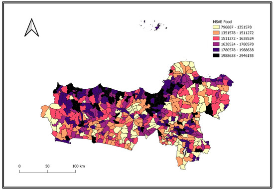
Figure 10.
Map of Estimation of Average Household Expenditure on Food at Subdistrict Level in Central Java using the Multivariate EBLUP Method.
Figure 10 also shows sub-districts with low average household expenditure on food, including sub-districts Paranggupito, Giritontro, Karangtengah, Tirtomoyo, Baturetno, Eromoko, Manyaran, Kismantoro, Bulukerto, and Jatipurno in Wonogiri Regency; Kedungjati, Geyer, Kradenan, Ngaringan, and Tanggungharjo in Grobogan Regency; Kayen, Pucakwangi, Tlogowungu, and Dukuhseti in Pati Regency; and Bulu, Tlogomulyo, Kaloran, Ngadirejo, Jumo, Candiroto, Bejen, Tretep, and Wonoboyo in Temanggung Regency.
Sub-districts with high average household expenditure on non-food items are generally located in urban areas, including South Magelang, Central Magelang, and North Magelang in Magelang city; Laweyan, Serengan, Pasar Kliwon, Jebres, and Banjarsari in Surakarta city; Argomulyo, Tingkir, Sidomukti, and Sidorejo sub-districts in Salatiga city; West Pekalongan, East Pekalongan, and North Pekalongan in Pekalongan city; South Tegal, East Tegal, and West Tegal in Tegal city; and almost all sub-districts in Semarang city (Figure 11). Meanwhile, sub-districts with low average food expenditure also tend to have low average non-food expenditure.
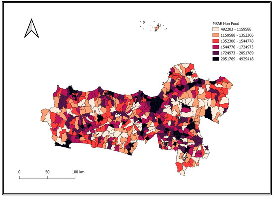
Figure 11.
Map of Estimation of Average Household Expenditure on Non-Food at the Sub-district Level in Central Java using the Multivariate EBLUP Method.
4. Discussion
The results of the estimation of the average household expenditure on food and non-food at the sub-district level in Central Java from the EBLUP-Fay–Herriot Multivariate model produced a better level of diversity than the direct estimation results. It can be seen from the comparison between the Relative Standard Error (RSE) value between direct estimation and the EBLUP Multivariate model for each sub-district in Central Java. Many outliers are still found in the box plot of the direct estimation results RSE value, and the RSE value is greater than 25 percent. Meanwhile, the EBLUP-Fay–Herriot Multivariate SAE results can significantly reduce the number of outliers in the RSE value. There are not even outliers at all in the RSE value of the EBLUP Multivariate estimation results for the average household expenditure variable for food in each sub-district. This result is in line with studies about EBLUP Multivariate that show the effectiveness of the EBLUP Multivariate method in producing estimates down to the smallest area level (sub-district). The EBLUP multivariate method outperforms direct estimation based on the survey design.
For the three sub-districts that were not sampled in the March 2020 National Socio-Economic Survey (Susenas), the average household expenditure on food and non-food was estimated by adding cluster information to the EBLUP-Fay–Herriot Multivariate. Table 6 shows that the estimated average household expenditure on food in Padureso sub-district is IDR 1,550,241, in Batuwarno sub-district it is IDR 1,574,599, and in Lebakbarang sub-district it is IDR 1,540,425. These three sub-districts are all members of cluster 1 for the average food expenditure variable group. Meanwhile, the estimated average household expenditure on non-food items in the three non-sampled sub-districts is lower than the value of food expenditure, namely IDR 1,470,115 in Padureso, IDR 1,455,223 in Batuwarno, and IDR 1,416,978 in Lebakbarang.
The Multivariate EBLUP estimation with the addition of cluster information can be used to estimate average household expenditure data down to the sub-district level, which can then be used as an indicator to categorize sub-districts in a region based on expenditure groupings. The estimated data can also be used as an indication or a reference in identifying priority regions to get targeted locations in programs for reducing poverty or improving community welfare. Through direct estimation of the survey design, it is impossible to collect statistics on average household expenditures down to the sub-district level. It is because the BPS survey has a limited budget and people to survey. This issue can be solved by using small area estimation using the EBLUP Multivariate approach and adding cluster information for areas not sampled in the survey. As a result, local government’s activities are more effective and focused since data is available down to the small area (subdistrict) level.
For future research, the use of the EBLUP Fay–Herriot Multivariate model can be applied to other data that has a strong correlation. If the research is conducted in areas that have different geographical characteristics, researchers can also develop the Fay–Herriot Multivariate model by adding spatial and time aspects. The auxiliary variables used can be differentiated in each research area because the influence of variables can be different in different areas, so it is expected that the estimation model formed will be better and more accurate. In addition, other clustering methods can also be used as alternatives in estimating unsampled areas, such as the Fuzzy K-Means non-hierarchical cluster method, Fuzzy K-Medoids, or hierarchical cluster methods.
5. Conclusions
The EBLUP-Fay–Herriot Multivariate method can improve the parameter estimates generated by the direct estimation method since it yields lower levels of variance (RSE) when estimating average household expenditure on food and non-food at the sub-district level for the sampled sub-districts in Central Java Province, Indonesia. For the sub-districts in Central Java Province that were not sampled from the March 2020 Susenas, the application of the EBLUP-Fay–Herriot multivariate method with the addition of K-Medoids cluster information can be done to estimate the average household expenditure for food and non-food at the sub-district level. The RSE value of all sub-districts from the EBLUP-Fay–Herriot Multivariate estimation is also below 25 percent, so the estimation results are reliable and provide a good level of diversity.
This research is expected to contribute significantly to multivariate modeling of the small area estimation level area. Additionally, it is envisaged that regional governments will use the information on average household expenditure at the sub-district level that results from the estimation using the Multivariate EBLUP-FH approach to design and implement programs relating to welfare and poverty. Because of the limited number of samples and budget, BPS, as the official statistics provider, is unable to provide this data down to the sub-district level.
Author Contributions
Writing (original draft), A.D., I.G., and T.T. All authors have read and agreed to the published version of the manuscript.
Funding
This research was supported by the Acceleration of Associate Professor Research (RPLK) Padjadjaran University 2022 Number 2203/UN6.3.1/PT.00/2022 and The APC was funded by DRPM of Padjadjaran University.
Data Availability Statement
Not applicable.
Conflicts of Interest
The authors declare no conflict of interest.
Appendix A
Table A1.
All Candidate Auxiliary Variables that Will Be Selected for EBLUP Multivariate Model.
Table A1.
All Candidate Auxiliary Variables that Will Be Selected for EBLUP Multivariate Model.
| No. | Variable Notation | Data | Source |
|---|---|---|---|
| (1) | (2) | (3) | (4) |
| Response Variable | |||
| 1 | Average household food consumption expenditure at sub-district level (IDR) | SUSENAS March 2020 | |
| 2 | Average household non-food consumption expenditure at sub-district level (IDR) | SUSENAS March 2020 | |
| Auxiliary variables | |||
| Population | |||
| 3 | Number of families using electricity (PLN and Non-PLN) | PODES 2020 | |
| 4 | Number of house buildings in slums | PODES 2020 | |
| Education | |||
| 5 | Number of elementary/islamic elementary Schools | PODES 2020 | |
| 6 | Number of junior high/islamic junior high Schools | PODES 2020 | |
| 7 | Number of high schools/islamic high schools | PODES 2020 | |
| 8 | Number of vocational schools | PODES 2020 | |
| 9 | Number of universities/colleges | PODES 2020 | |
| Health | |||
| 10 | Number of maternity hospitals | PODES 2020 | |
| 11 | Number of health centers with inpatient care | PODES 2020 | |
| 12 | Number of health centers without inpatient care | PODES 2020 | |
| 13 | Number of auxiliary health centers | PODES 2020 | |
| 14 | Number of polyclinics/treatment centers | PODES 2020 | |
| 15 | Number of doctor’s offices | PODES 2020 | |
| 16 | Number of maternity homes | PODES 2020 | |
| 17 | Number of midwife practice sites | PODES 2020 | |
| 18 | Number of village health posts (poskesdes) | PODES 2020 | |
| 19 | Number of village maternity clinics (Polindes) | PODES 2020 | |
| 20 | Number of pharmacies | PODES 2020 | |
| 21 | Number of specialty medicine/herbal shops | PODES 2020 | |
| Economy (Industry) | |||
| 22 | Number of small and medium industries (IMK) of leather | PODES 2020 | |
| 23 | Number of small and medium industries (IMK) of wood | PODES 2020 | |
| 24 | Number of small and medium industries (IMK) of precious metals or metal materials | PODES 2020 | |
| 25 | Number of small and medium industries (IMK) of fabric/weaving | PODES 2020 | |
| 26 | Number of small and medium industries (IMK) of pottery/ceramics/stone | PODES 2020 | |
| 27 | Number of small and medium industries (IMK) from rattan/bamboo, grass, pandanus, etc. | PODES 2020 | |
| 28 | Number of small and medium industries (IMK) of food and beverages | PODES 2020 | |
| 29 | Number of other small and medium industries (IMK) | PODES 2020 | |
| Economy (Other than Industry) | |||
| 30 | Number of shop groups | PODES 2020 | |
| 31 | Number of markets with permanent buildings | PODES 2020 | |
| 32 | Number of markets with semi-permanent buildings | PODES 2020 | |
| 33 | Number of markets without buildings | PODES 2020 | |
| 34 | Number of minimarkets/supermarkets | PODES 2020 | |
| 35 | Number of shops/grocery stores | PODES 2020 | |
| 36 | Number of restaurants/dining houses | PODES 2020 | |
| 37 | Number of food and beverage stalls | PODES 2020 | |
| 38 | Number of hotels | PODES 2020 | |
| 39 | Number of lodgings | PODES 2020 | |
| Economy (Financial Inclusiveness) | |||
| 40 | Number of state-owned commercial banks | PODES 2020 | |
| 41 | Number of private commercial banks | PODES 2020 | |
| 42 | Number of rural banks | PODES 2020 | |
Appendix B
Table A2.
Two Stage One Phase Sampling for March 2020 National Socio-Economic Survey.
Table A2.
Two Stage One Phase Sampling for March 2020 National Socio-Economic Survey.
| Phase | Unit | The Number of Units of the-h Strata | Sampling Method | Possibilities for Sample Selection | Sampling Fraction | |
|---|---|---|---|---|---|---|
| Population | Sample | |||||
| 1 | Census Block | PPS-with replacement | ||||
| Systematic | ||||||
| 2 | Household | Systematic | ||||
with:
- number of census blocks in the -th strata of the -th district
- 40% of the total census block in the -th strata of the -th district
- number of samples of the March Susenas census blocks in the -th strata of the -th district
- : total household load of the -th strata of the -th district SP2020 data
- : total load of households in the -th census block, -th stratum, -th district SP2020
- : the number of household contents in the -th updated census block, -th stratum, -th district
- : number of household samples in each census block
If there are sub-districts in a population and sub-districts are sampled randomly, and household expenditure is available for each -th household in sub-district, then the average household expenditure of a sub-district is calculated by the formula:
with:
- : the average expenditure of households in the -th sub-district
- total expenditure of the -th household in the -th sub-district
- : the weighting factor of the -th household in the -th sub-district obtained from the March Susenas sampling design
- : the number of households in the -th sub-district
- : number of the sub-districts
References
- Sekhampu, T.J.; Niyimbanira, F. Analysis of the Factors Influencing Household Expenditure In A South African Township. Int. Bus. Econ. Res. J. 2013, 12, 279. [Google Scholar] [CrossRef][Green Version]
- Irawan, P.B.; Usman, H. Official Statistics: Sosial Kependudukan Dasar; Media: Bogor, Indonesia, 2016. [Google Scholar]
- Kurnia, A.; Notodiputro, K.A. Eb-Eblup Mse Estimator on Small Area Estimation with Application to BPS Data. In Proceedings of the First International Conference on Mathematics and Statistics (ICoMS-1), Bandung, Indonesia, 19–21 June 2006; pp. 1–6. [Google Scholar]
- Rao, J.N.K.; Molina, I. Small Area Estimation, 2nd ed.; John Wiley & Sons: New York, NY, USA, 2015. [Google Scholar]
- Ghosh, M.; Rao, J.N.K. Small area estimation: An appraisal. Stat. Sci. 1994, 9, 55–76. [Google Scholar] [CrossRef]
- Fay, R.E., III; Herriot, R.A. Estimates of Income for Small Places: An Application of James-Stein Procedures to Census Data. J. Am. Stat. Assoc. 1979, 74, 269. [Google Scholar] [CrossRef]
- Nurizza, W.A. Penerapan Model Fay-Heriot Multivariat Pada Small Area Estimation (Studi Simulasi Pengeluaran Rumah Tangga per Kapita di Indonesia Tahun 2017) [Skripsi]; STIS: Jakarta, Indonesia, 2018. [Google Scholar]
- Ghosh, M. Small area estimation: Its evolution in five decades. Stat. Transit. New Ser. 2020, 21, 1–22. [Google Scholar] [CrossRef]
- Benavent, R.; Morales, D. Multivariate Fay-Herriot models for small area estimation. Comput. Stat. Data Anal. 2016, 94, 372–390. [Google Scholar] [CrossRef]
- BPS. Pengeluaran per Kapita, Sirusa. 2021. Available online: https://sirusa.bps.go.id/sirusa/index.php/indikator/197 (accessed on 1 June 2022).
- Rao, J.N.K. Some Recent Advances in Model- Based Small Area Estimation. Surv. Methodol. 1999, 25, 175–186. [Google Scholar]
- Saei, A.; Chambers, R. Small Area Estimation: A Review of Methods Based on the Application of Mixed Models; University of Southampton: Highfield, UK, 2003. [Google Scholar]
- Ginanjar, I.; Iaeng, M.; Wulandary, S.; Toharudin, T. Empirical Best Linear Unbiased Prediction Method with K-Medoids Cluster for Estimate Per Capita Expenditure of Sub-District Level. IAENG Int. J. Appl. Math. 2022, 52, 3. [Google Scholar]
- Anisa, R.; Kurnia, A.; Indahwati, I. Cluster Information of Non-Sampled Area In Small Area Estimation. IOSR J. Math. 2014, 19, 15–19. [Google Scholar] [CrossRef]
- Nuryadin, H.; Susetyo, B.; Sadik, K. Application of Small Area Estimation of Multivariate Fay-Herriot Model for The Average of Per Capita Expeniture in Village Level. Int. J. Sci. Eng. 2017, 8, 1673–1676. [Google Scholar]
- Patel, A.; Singh, P. New Approach for K-mean and K-medoids Algorithm. Int. J. Comput. Appl. Technol. Res. 2012, 2, 1–5. [Google Scholar] [CrossRef]
- Sangga, V.A.P. Perbandingan Algoritma K-Means dan Algoritma K-Medoids dalam Pengelompokan Komoditas Peternakan di Provinsi Jawa Tengah Tahun 2015. Tugas Akhir Jur. Stat. Fak. Mat. dan Ilmu Pengetah. Alam Univ. Islam Inndonesia Yogyakarta 2018, 53, 1689–1699. [Google Scholar]
- Rao, J.N.K. Small Area Estimation; Wiley: Hoboken, NJ, USA, 2003. [Google Scholar]
- Desiyanti, A.; Toharudin, T.; Suparman, Y. The Implementation of Empirical Best Linear Unbiased Prediction-Fay Herriot (EBLUP-FH) on the Estimation of Average per Capita Expenditure at District Level in West Sumatra Province in 2019. J. Math. Comput. Sci. 2022, 12. [Google Scholar] [CrossRef]
- Amaliana, L.; Fithriani, I.; Siswantining, T. Pendugaan Mean Squared Error (Mse) Pada Model Fay-Herriot Small Area Estimation (Sae). Pros. Semin. Nas. Mat. Dan Pembelajarannya 2017, 9, 205–212. [Google Scholar]
- Nurizza, W.A.; Ubaidillah, A. A comparative study of multivariate Fay-Herriot model for small area estimation in various sample sizes. IOP Conf. Ser. Earth Environ. Sci. 2019, 299, 12027. [Google Scholar] [CrossRef]
- Pfeffermann, D. New important developments in small area estimation. Stat. Sci. 2013, 28, 40–68. [Google Scholar] [CrossRef]
- Ubaidillah, A. Simultaneous Equation Models for Small Area Estimation. Ph.D. Thesis, Bogor Agricultural University, Bogor, Indonesia, 2017. [Google Scholar] [CrossRef]
- Patterson, H.D.; Thompson, R. Recovery of Inter-Block Information when Block Sizes are Unequal. Biometrika 1971, 58, 545. [Google Scholar] [CrossRef]
- De Vaus, D. Surveys in Social Research, 5th ed.; Allen and Unwin: Crows Nest, NSW, Australia, 2002. [Google Scholar]


Disclaimer/Publisher’s Note: The statements, opinions and data contained in all publications are solely those of the individual author(s) and contributor(s) and not of MDPI and/or the editor(s). MDPI and/or the editor(s) disclaim responsibility for any injury to people or property resulting from any ideas, methods, instructions or products referred to in the content. |
© 2022 by the authors. Licensee MDPI, Basel, Switzerland. This article is an open access article distributed under the terms and conditions of the Creative Commons Attribution (CC BY) license (https://creativecommons.org/licenses/by/4.0/).