1. Introduction
Nowadays the electrical network is continuously evolving due to consumers demand, to increase the deployment of system information technologies and due to the diversity of available energy resources, facts that directly affect the quality of the electricity distribution service, respectively, have a direct impact on the energy supplied to large consumers, regarding quality and amount of delivered energy [
1,
2,
3]. For this reason, the quality of distributed electricity is an important concern, and ensuring the quality of delivered electricity causes the power grid to evolve into a smart grid [
4,
5,
6,
7]. Power quality is defined and simplified, by three important aspects: availability, wave quality, and commercial quality. From the distribution network operator point of view, availability is a very important point in order to maintain a high level of reliability. For this reason, the detection of a fault is a priority for the electric network operator, in order to provide a high level of reliability in supplying energy to consumers [
2].
Monitoring the electrical parameters of the network allows to distinguish between the normal operating regime and the appearance of a fault or abnormal operation of the network, whereby they undergo substantial changes such as:
Increasing current and decreasing phase voltage, and as a consequence the reducing of the impedance between the measurement point and the fault location;
Increase or decrease voltage as a result of switching;
Frequency oscillations;
Increase temperature of current paths.
Protection and fault detection functions are performed by supervising the deviations of the system parameters [
8,
9,
10,
11,
12].
The paper [
13] mentions the need to improve the protection of power lines and analyzes the function of overhead power lines, in front of a fault, from the point of view of external factor influence on distance protection. In order to develop an intelligent system for distance protection with adaptive algorithms the work takes into account changes in climatic factors to increase the protection sensitivity. The work seeks ways to increase the stability of OPL operation by developing new algorithms for determining fault detection based not only on measuring operating parameters but also based on external environmental parameters such as ambient temperature, air humidity, wind speed, and soil moisture under the studied overhead power line. In case of a fault on the protected line, data are received from current and voltage transformers. Fault values are compared with the protection setpoints and the protection is activated, this being the standard mode of operation described in our manuscript. Compared to our work this proposed algorithm proves useful in determining the fault location but does not speed up protection timing resulting in the same exposure to fault values, without the added benefits of using a control structure for rapid identification of a fault and triggering of the line protection relay. Today’s relays are predominantly based on phasors, and as such, they encounter a delay associated with the full cycle observation window required for accurate fault detection, thus, [
14] reviews a number of protection techniques that have the potential to significantly speed up line protection.
The automatic protection systems of the 110 kV power line, analyzed in this document, allowed the recording of events that occurred over time, providing the basic knowledge for fault analysis and a clear view of the event in time. These protection systems are located in 110/20 kV substations, at both ends of the interconnection lines. Instrumentation of the fault values was carried out using dedicated software, which allowed the connection to data recorded by the perturbograph of a protection system, namely a digital terminal. The causes, magnitude, and consequences of the fault on the power network were estimated using this software.
Distance protection is currently the basic element used in protection systems for 110 kV power lines.
The main advantages of distance protection are:
Reduced dependence of sensitivity on the operating regime of the network;
Disconnection of faults with a shorter delay, the closer they occur to the place of installation of the relay;
Delimitation of protected areas with sufficient precision.
As a working principle, in the event of a fault, the distance protection measures the impedance between the installation location and the short circuit location. The distance module successively compares the measured values with the impedances set on the relay. The impedances set as the operating parameters of the protection reflect the length of the protected zones, usually divided into four steps. Impedance is the ratio of the amplitudes of voltage and current flowing, along the power line [
13,
14].
However, conventional distance protection faces several drawbacks that might lead to maloperation, according to [
15], and thus new methods to estimate the distance to the fault in the presence of infeed from alternative power sources such as solar, wind, and batteries are proposed. The aim is to improve line protection based on local measurements and offline calculations, but such work does not use mathematical models or neural network models to evaluate the nature of the fault and to obtain a faster reaction of the line protection, as the problem is going to be approached in the current paper, thus the obtained results indicate just the potential of avoiding maloperation of distance relays in power systems.
One must be able to precisely forecast how various components of the grid, such as transformers, transmission power lines, cables, substations, etc., will operate to effectively simulate the behavior of the overall grid. This often indicates that there are two options available: the first is to have a holistic model that properly explains the observed data, and the second is to have a physical model of that specific network piece [
15,
16]. This work focused on holistic modeling, and to obtain such a model the primary categories of mathematical approaches include empirical, analytical, numerical, or a mix of them. Experimental values are described, and then frequently used mathematical equations are modified to match the experimental data, as is the case with empirical approaches. Mathematical formulations are utilized in analytical approaches to completely explain the simulations, but when this is not feasible, numerical estimations are used [
17,
18,
19]. Tools can be used in the context of model-based systems engineering to be able to control data by suitable systems so that the processing of these data can be accomplished by many developers in a distributed development environment [
20]. Model-based system engineering supports a variety of practical modeling techniques including experimental identification, and deals with the design of complex systems and mostly generates point solutions. The objectives are to incorporate the outcomes of many development efforts into a central model of the system [
21,
22].
Understanding the precise causes of power line failures enables more effective control of the whole network since the high dependability of power transmission lines is one of the key factors that ensures network stability over time [
23]. Given these details, it is desirable to model the transmission power lines, which, in addition to offering the chance to confirm any fault occurrence, offer extra significant advantages. The obtained model is appropriate for testing the actual likelihood of a transient or persistent fault occurring [
24].
Faults are divided according to their nature into transient and persistent faults. The main difference between the two types of faults presented as case studies is the duration of the fault or event in the network. Transient faults are cleared by the automatic system in a very short time, compared to persistent faults that require an intervention for the physical repair of the network. Transient faults usually involve momentary vegetation contact, bird or animal contact and are referred to as temporary events, while persistent faults, also referred to as permanent events, are caused by insulation failure of live conductors, broken conductors, or some sort of mechanical damage.
Ref. [
25] describes the function of a protective relay for fast and reliable transmission line protection that responds to transient and permanent conditions or transient and persistent faults. A concept of the dual filter scheme developed based on the principle of multiple data-window filters, combining voltage and current data from half-cycle and one-cycle windows to obtain distance element detection and achieve fast tripping times was also presented. Using mathematical calculations and relay voltage and current phasors particular to an impedance loop six impedance loops were necessary to detect all faults. An algorithm that calculates three incremental torques of voltages and currents, between phases, to determine the fault was required to support the selectivity of tripping due to the instability of the phasors. However, the gain in time due to the application of the concept was not specified, only the compared results from using different detection methods were mentioned.
If one needs to identify the transfer function based on observed values of transient and persistent faults, that destabilize a known distribution system, an experimentally identified model can prove very useful. The fact that all pertinent system data are gathered in a comprehensive system model makes experimental identification significantly superior to a document-based method [
20].
Therefore, the first goal of this document is to develop a mathematical model that establishes the occurrence of a fault, with high precision, by analyzing the voltage and current waves that make up the impedance of the power line, with the purpose of enhancing the stability of the electrical distribution networks, and in a second term to establish a procedure that allows for a quicker response regarding fault clearing time in order to obtain improved triggering properties in protective devices. A graphical comparison of the developed model’s predictions with the experimental data intends to demonstrate the model’s correctness.
Other methods of fault clearing involve overcurrent protection with minimum voltage blocking or low-voltage protection conditioned by overcurrent protection. These methods do not offer sufficient selective high-speed clearance of faults on high voltage power lines and therefore are not taken into consideration, as faults must be triggered faster than a critical fault clearing time or else power line damage might occur, and the system could lose stability and possibly even blackout [
24,
25].
Due to actual consumer demand, the use of new smart technologies present in household electrical appliances, and every industrial process, interruptions in electricity supply pose significant economic and social impact. Power line protection technology has to suit this new way of life, power lines being the main arteries of the distribution system and every short circuit that occurs here impacts the whole system affecting a large number of consumers.
Speed is one of the most important conditions that must be met by protection systems, especially those mounted on high voltages, which are complex systems with a wide coverage area and high powers.
In front of this scenario, it is very important to introduce a new kind of method which aims to rapidly clear a fault and then create the path to establish a fast network restoration. There is a need to reduce the time of exposure to the fault effects, by increasing the reaction speed of the protection systems, providing the necessary selectivity, in order to increase the continuity and stability of electricity delivered to consumers.
3. Mathematical Models for Experimental Response Determination in Voltage and Current for Transient and Permanent Faults
To accurately determine the experimental response of the propagation of a single-phase earth fault, several real situations were analyzed, including the transient fault that is the subject of the case study, which appeared on the 110 kV line.
The case study was carried out for:
Installation: 110 kV OPL Fântânele-Târnăveni, Romania (overhead power line);
Event: Transient fault, on phase R, triggered by distance protection, cleared by automatic reclosing.
The oscillogram of events shows the appearance and evolution of the fault, until the tripping of the power line by the distance protection and is presented in
Figure 1. With the help of the perturbograph, the values sampled every millisecond were analyzed, with the observation of the single-phase fault propagation tendency every 5 ms to determine the experimental response of the process in case of the presented event.
In normal operation mode, the amplitude of the voltage signal in
Figure 1 is 58.63 V, corresponding to approximately 110 kV line voltage measured in the primary of the voltage transformer, an amplitude that decreases progressively during fault propagation, until the tripping of the line at 120 ms. It then reaches 1.33 V in failure mode. The time of 0 ms marks the activation of the distance protection, the moment when the fault is detected. The phenomenon of occurrence of the fault is visible in the time interval [−20; 20] ms, a time interval of 40 ms that will be later taken into consideration. Amplitude for the current signal, in normal operation mode, shown in
Figure 1 is 2.95 A, an amplitude that increases progressively when the fault appears until it stabilizes (in the fault regime) at around 10 A secondary current, corresponding to 1200 A primary current, a value that endangers the structure of the power line. The phenomenon that takes place during the appearance of the fault is visible in a 40 ms time interval [−20; 20] ms, which is relevant for the experimental response and therefore referred to in the next figures.
In
Figure 2 the experimental response for a transient fault is presented, namely the variation of the effective value of the V
R voltage with respect to time V
R(t). The experimental values were taken using the Δt = 1 ms sample and captured the appearance of the fault.
The slightly “deformed” shape of the experimental curve is due to the relatively high value, in the context of the present application, of the experimental data sampling step. In order to obtain the possibility of applying the identification methods of the mathematical model that describes the propagation of the fault, it is necessary to approximate, based on the experimental response the most probable response [
26,
27,
28]. In this context, the experimental response is approximated by using a polynomial curve of the 7th degree.
The relation of the approximating polynomial of the 7th degree is:
where the coefficients are:
,
,
,
,
,
,
, and
.
The comparative graph between the experimental response and the response of the determined polynomial model is presented in
Figure 3. The figure shows a faithful superposition of the two curves, the response of the approximating polynomial model accurately reproducing the dynamics of the experimental response. Practically, the response of the approximating polynomial model has the appearance of the filtered experimental response. This aspect demonstrates the high quality of the identified polynomial model.
The presence of the inflection point, in the case of the approximating polynomial model response shown in
Figure 3 implies higher-order dynamics for fault propagation. In order to identify the time constants of the propagation process, the tangent method is applied based on the approximate polynomial response. Application of the tangent method to identify the dynamics of fault propagation is presented in
Figure 4 [
29,
30].
A tangent line is applied at the inflection point i. The intersection of the tangent with the time axis parallel that passes through the initial value of the response (yi = 58.63 V) occurs at t1 = 5.9 ms, and the intersection of the tangent with the time axis parallel that passes through the final value (the steady state) of the response (yf = 20.45 V) occurs at t2 = 17.9 ms.
The mathematical model that describes the defect propagation can be expressed in the form of a second-order transfer function (representing the simplest form of a higher-order model) [
31,
32,
33,
34]. The input signal that produces the variations of the output signal presented in previous figures is considered to be a unitary step (u(t) = 1; U(s) = L{u(t)} = 1/s) having the physical meaning of the event that triggered the fault. The proportionality constant of the process is given by the mathematical expression of this index:
where u
0 = 1 represents the variation of the input signal (from the initial value 0 to the value associated with the occurrence of the event that triggered the fault, value quantified as 1). The result is the value of the proportionality constant of the process K = −38.18 V.
The sum of the two time constants T
1 and T
2 of the second-order transfer function, representing the mathematical model of the process, is given by:
resulting in:
.
By expressing the output signal
, this will be given by the equation:
−1, where:
The optimal solution for the values of the two time constants of the addressed process is examined in the context of considering only non-zero integer values for the two and taking into account that
. The answers of some of the models obtained by considering a few of the possible pairs of values for T
1 and T
2 are depicted in
Figure 5.
From
Figure 5, it turns out that the response that most faithfully reproduces the experimental response of the process is obtained for T
1 = T
2 = 6 ms. This conclusion results from the analysis of every possible combination of values of T
1 and T
2. Consequently, the final form of the identified transfer function H(s) based on the relation of the proposed second-order mathematical model is:
Due to the high accuracy provided by the identified model, its refinement by considering some rational values for the two time constants of the fault propagation process is not justified.
Another possibility for identifying the fault propagation process is based on the use of Gaussian models. The relation of the Gaussian function, usable for identifying the dynamics of fault propagation, is:
where T is the time constant of the process. Moreover, y
G(t) represents the notation of the output signal V
R(t) in the variant of using the Gaussian model and K and y
i have the same meaning and value as in the case of using the second-order model. An iterative procedure is applied to determine the time constant T of the defect propagation process.
The step responses of the models obtained by considering different values for the time constant T are presented in
Figure 6. The values of the time constant used to determine the curves in
Figure 6 were: T = 13.035 ms (T
2 = 170 [ms]
2); T = 13.784 ms (T
2 = 190 [ms]
2); T = 14.491 ms (T
2 = 210 [ms]
2). The three determined models generate similar performances, of which the mathematical model in which T
2 = 190 [ms]
2 is considered to generate the highest accuracy. Since the performance improvement generated by the Gaussian model when T
2 varies around 190 [ms]
2 is not significant, refining the model by fine-tuning T
2 is not justified.
An important stage of the research consists in comparing the performances generated by the two types of mathematical models identified. In this context, in
Figure 7, the comparative graph is presented between the experimental response and the responses of the two types of mathematical models proposed in the variants that generated the best performances, respectively, the variant in which T
1 = T
2 = 6 ms in the case of the second-order mathematical model and the variant in which T
2 = 190 [ms]
2 in the case of the Gaussian mathematical model.
From
Figure 7, it follows that the proposed Gaussian mathematical model ensures a higher accuracy than the mathematical model of the second order, the related response being closer to the dynamics of the experimental response.
Another important problem is represented by the need for mathematical modeling of the intensity of the electric current I
R(t) associated with phase R. The dynamics of the I
R(t) signal, obtained experimentally, are presented in
Figure 8.
As in the case of V
R(t) voltage, the experimental response is approximated by using a polynomial curve of the 4th degree. The equation of the approximating polynomial of the 4th degree is as follows:
where the coefficients are: p
4 = 4.033 × 10
−5, p
3 = −0.0031575, p
2 = 0.06485, p
1 = 0.028559 and p
0 = 2.9577.
The comparative graph between the experimental response I
R(t) and the response of the approximating polynomial model is presented in
Figure 9.
Results presented in
Figure 9 show that the dynamics of the approximate polynomial response follow with high accuracy the dynamics of the experimental response, an aspect that demonstrates a good quality of the performed identification. Moreover, the data from
Figure 8 and
Figure 9 result from the fact that the dynamics of the I
R(t) signal in the regime of the appearance of the defect show overshoot.
The mathematical modeling of the dynamics of the I
R(t) signal in the fault propagation regime is performed using the same principle as in the case of the voltage V
R(t), with the difference that H(s) takes the form [
30,
31]:
where
represents the damping factor, and ω
n represents the natural pulsation.
The following experimental values (associated with the experimental response) are considered: the initial value of the experimental response −y
0 = 2.953 A; the maximum value of the experimental response −y
max = 10.69 A; the steady state value of the experimental response −y
st = 8.66 A. Using these experimental values, the overshoot of the I
R(t) signal can be computed, using the mathematical expression:
From (9), it results that the overregulation expressed in percentage is equal to 35.58%. Knowing the value of the overshoot, the damping factor can be computed using the expression:
Analyzing the experimental data, it follows that the response time of the I
R(t) signal in the fault propagation regime is approximately t
r = 80 ms. In this context, the following expression can be written:
from which the initial value of the natural pulse can be deduced:
Moreover, to obtain a slightly higher precision, the value of the natural pulsation obtained in relation (12) was slightly adjusted, its final value identified being:
In conclusion, the transfer function representing the mathematical model of the fault propagation phenomenon associated with the I
R(t) signal, can be extracted from the Equation (8) by specifying the structure parameters of the initial transfer function:
In
Figure 10, the comparative graph is presented between the experimental response, respectively, the approximating polynomial model response and the proposed second-order mathematical model response, related to the dynamics of the I
R(t) signal.
Figure 10 presents the validity of the mathematical model proposed in relation (14), where the dynamics of its response follow with high accuracy the dynamics of the other two responses.
The advantage of the second-order model proposed in relation to the polynomial model is its generality in the sense that it retains its validity outside the considered time domain. The approximating polynomial model is valid only in the considered time domain and is useful for the application of identification procedures.
The second case study was carried out for:
Installation: 110 kV OPL Fântânele-Târnăveni, Romania;
Event: Persistent fault, broken line conductor, on phase R, triggered by distance protection, automatic reclosing failed.
By analyzing the fault values and the mode of operation of the protection, we identified the particularities of the event caused by the breaking of the conductor, a serious defect that led to the unavailability of the line. The oscillogram of the event is shown in
Figure 11.
In
Figure 11, the oscillogram of the event presents the appearance of the fault. In normal operation, t = −150 ms, 150 ms before the fault the recorded currents and voltages are of normal values, on all three phases referred to as R, S, T, there is virtually no homopolar current (IH) meaning there is no earth fault. At the point marked with 0 ms, the fault is recorded with the values presented in the right column of the oscillogram, at the moment t = 0 ms. At the moment of the appearance of the fault on the R phase, we found a dangerous increase in the current recorded on the R phase (IR) and a sharp decrease in the UR voltage, which tends to zero, as the fault progresses. Healthy phases S and T experience increases in currents and voltages a fact that constitutes an additional danger for the integrity of the installations and consumers. The break of the active conductor and its fall to the ground causes the appearance of the homopolar current and the voltage (IH and UH) recorded with high values, at the time the fault is detected. The line circuit breaker is closed, a fact marked by the red line next to the INTR_CLO row and disconnects the line at time t = 130 ms, a fact marked with the INTR_OPE entry, thus further damage is stopped, by triggering the line through the distance protection.
In this case, the fault values are more pronounced than in the case of the transient defect presented previously.
The phenomenon of the appearance of the fault, on phase R, is also visible, here in a 40 ms time interval which will be taken into account below.
The experimental response for a persistent fault is shown in
Figure 12, respectively, the variation of the effective value of the V
R voltage (UR on the oscillogram) in relation to time V
R(t). Identical to the previous case of the transient fault presented earlier, the experimental values were taken using the sample of
and captured the appearance of the fault.
The mathematical model determined for this event has the same form as in the previous case, with the only difference that the transfer function is of order III, having the structure:
where T
3 is the time constant of the fault propagation phenomenon. The proportionality constant K was determined using the relation (2), but using the experimental data related to the current case (the resulting value being K = −37.83 V), and the time constant T
3 was determined by applying an iterative procedure to minimize the quality indicator (mean square error) between the experimental response and the response of the proposed mathematical model (the resulting value being T
3 = 5.15 ms).
By applying the experimental identification procedure, the transfer function presented in the following equation was obtained:
The comparative graph between the experimental response and the response of the proposed third-order model, presented in
Figure 13, demonstrates a high quality of identification (the determined curve related to the response of the mathematical model follows the dynamics of the experimental curve with high accuracy).
Same as before, in the case addressed, the Gaussian mathematical model that describes the defect propagation phenomenon was identified. The Gaussian mathematical model preserves the structure presented in the previous case, the only difference being the re-identification of the structure parameters based on the new experimental data related to the experimental curve presented in
Figure 12. In this context, the proportionality constant K has the same meaning and value as in the case of relation (16), and the identified value for the time constant of the model is T
G = 17.32 ms (T
G2 = 300 [ms]
2).
The comparative graph between the experimental response and the response of the proposed Gaussian model is presented in
Figure 14, the conclusion regarding the quality of the identification being the same as that deduced in the case of
Figure 13.
In the following figure,
Figure 15, the comparative graph between the experimental response and the responses of the two types of determined mathematical models that describe the propagation of the fault occurring phenomenon (the third-order mathematical model, respectively, the Gaussian mathematical model) is presented.
By analyzing
Figure 15, the conclusion is that the two proposed mathematical models present approximately the same degree of accuracy.
For the addressed case, the dynamics of the I
R(t) experimentally obtained signal is presented in
Figure 16.
Keeping the same structure of the mathematical model as in the previous case (the case of the mathematical modeling of the intensity of the electric current I
R(t) associated with the phase R) and applying a similar identification procedure, a new form of the transfer function H(s) was determined, presented in (17):
The mathematical expression of the approximating polynomial that approximates the curve in
Figure 16 is identical to the one in (7), and the coefficients determined for the current case are: p
4 = −5.82 × 10
−6, p
3 = 0.0010599, p
2 = −0.058861, p
1 = 1.2345, respectively, p
0 = 2.0231.
The experimental response in relation to the approximating polynomial model response and the proposed second-order mathematical model response, related to the dynamics of the I
R(t) signal are presented in
Figure 17 through a comparative graph.
Figure 17 certifies the validity of the mathematical model proposed in relation (17) since the dynamics of its response follows the dynamics of the other two responses with high accuracy.
4. Structure for Rapid Fault Identification and Protection Relay Triggering
The structure of the automatic control structure proposed for the rapid identification of the fault occurrence and for triggering the protection relay [
26,
32], is presented in
Figure 18.
Figure 18 “Electric Power Distribution Process” refers to the power distribution lines acknowledged as the case study of this analysis. “Measuring equipment” is used to measure signals of interest for various applications. In the present approach, the measured signals of interest are the voltage V
R(t) and the current I
R(t).
The actual mechanism for rapid identification of the defect and command of the protection relay contains the following elements in its structure: “Signal Processing and Calculation Element”, “Reference Voltage Generator”, “Decision Element”, respectively, an Adder block that performs the subtraction of two derivatives of voltages in relation to time (VDRV(t) and VREF(t)) since the voltage derived in relation to time VREF(t) is applied to its input with the minus sign.
Either VR(t) or IR(t) can be considered as the main signal processed by the fast fault identification algorithm. This aspect is due to the fact that the two signals show strong variations in the fault propagation regime, respectively, the VR(t) signal shows a strong and monotonous decrease until stabilization, and the IR(t) signal shows a strong and monotonous increase until stabilization. If one of the two signals is chosen as the main signal, the other signal is used in the quick fault identification procedure as a support signal. In the proposed procedure, VR(t) is chosen as the main signal. The fact that the dynamics of the two signals VR(t) and IR(t) are used in the rapid fault identification procedure also represents the justification that they were mathematically modeled in the previously presented sections.
The procedure for quickly identifying the occurrence of the fault, respectively, for controlling the protection relay, follows the next steps:
The first step defines the effective working value of the voltage VR(t), respectively, the effective working value of the current IR(t);
Based on the mathematical models determined by using the three sets of experimental data associated with the three experimental procedures carried out, the time derivatives of the VR(t) signal are computed (distinct for the three mentioned cases; using Euler’s approximation);
It determines the minimum values of the three derivatives in relation to the corresponding time of the VR(t) signal, derivatives computed in step 2; the two identified minimum values are marked with V1, V2;
The arithmetical mean of the V1, V2 values previously determined in step 3 is computed, resulting in a mean value (Vmed);
The VR(t) signal values and the IR(t) signal values are monitored online;
If there are two consecutive increases in the error between the effective working value and the instantaneous effective value of VR(t), and at the same time two consecutive decreases in the error between the effective working value and the instantaneous effective value of IR(t), the derivative of the VR(t) signal with respect to time is computed using Euler’s approximation and its minimum value is determined;
If the minimum value of the derivative with respect to the time of the signal VR(t), computed in step 6 (value associated with the change in the monotony of the derivative) is less than 1/2 of the arithmetic mean of the values V1 and V2, then the occurrence of a fault is detected (the reference value for the mentioned comparison depends on the Hmed computed in step 4, and the weighting coefficient (in this case 1/2) can be modified according to the particularities and properties of the considered electricity distribution system.
It is very important to mention that steps 1 to 4 are applied only once for each commissioning of the rapid fault identification mechanism. Moreover, steps 5 and 6 apply for the entire operation of the electricity distribution process, and step 7 only applies if the constraint mentioned in step 6 is met. If step 7 is applied, and the constraint at this step is satisfied, basically the fault is detected, and the protection relay will be triggered. If the constraint from this step is not satisfied, it is considered that the variations in the VR(t) and IR(t) signals detected in step 6 are not due to a fault, but to other less significant causes that do not influence the proper functioning of the system. The procedure, in this case, is to continue applying steps 5 and 6 until step 7 is reached again.
It is also very important to mention that, in the case of the rapid fault identification mechanism, when referring to the V
R(t) and I
R(t) signals, the dynamics of their actual values are considered, not the actual sinusoidal dynamics. The parameters mentioned in step 1 are defined within the “Signal processing and calculation element”. Step 2 allows the calculation of the time derivative of the V
R(t) signal in the three experimental cases. In this context, the time derivative of the signal V
R(t), in the general case, is computed using Euler’s method by applying the following expression:
where V
DRV(t
i) represents the time derivative of the signal V
R(t),
, at the moment t
i belonging to the time domain related to the operation of the electrical energy distribution process and T
h represents the approximation step of the derivative (constant step). For a precise representation of the V
DRV(t) derivative, a very small approximation step (compared to Δt) was chosen, namely
. Although the approximation step is smaller than the experimental data sampling period, the derivative V
DRV(t) can be computed by using the mathematical models determined in the previous sections.
Using the Gaussian mathematical model and expression (18), it is possible to calculate the first-order derivative of the V
R(t) signal in relation to time, its dynamics (also in relation to time) being presented in
Figure 19 for the case of the transient fault (the first case study), respectively, in
Figure 20 for the case of the persistent fault (the second case study).
Due to the very close accuracy in terms of value (obtained in the presented two cases) generated by the Gaussian models in relation to those that use transfer functions, in the case of using the last mentioned for calculating the derivative values, the results obtained are very close (without significantly modifying the forms of variation, respectively, derivative values with respect to time).
Using the curves from
Figure 19 and
Figure 20, step 3 of the quick fault identification procedure can be applied, the minimum values of the two derivations in relation to the time of the V
R(t) signal, being: V
1 = −2.5117 V/s (obtained at t
1 = 9.2 ms), respectively, V
2 = −1.8734 V/s (obtained at t
2 = 12.1 ms).
The fact that the mathematical models proposed for rendering the fault propagation phenomenon allowed the use of the approximation step Th = Δt/10 = 0.1 ms, makes for the high accuracy of the calculation of the derivatives previously presented. If the approximation step used would have equal Δt, the accuracy of the representation would have been much lower since the density of samples used would have been 10 times lower. Also in this context, the direct use of experimental data regarding the calculation of the derivative would have generated even weaker results based on the same explanation as the previous one, but also due to the distorted aspect of the experimental curves. This aspect is due both to the large sampling step of the experimental data, as well as of the measurement errors, respectively, of the fact that the effect of the defect propagates.
In
Figure 19 and
Figure 20, a scaling with 10
3 is shown on the ordinate since the approximation step T
h is expressed in ms (thereby making the conversion in seconds). Knowing the values of V
1 and V
2, we can proceed to step 4 by calculating the arithmetic mean of the two values, which is: V
med = −2.19255 V/s.
Step 6 of the fast fault detection algorithm is implemented by the “Signal Processing and Computing Element”. The signal processing component manages the detection process, and it is responsible for the detection of two consecutive increases in the value of the error between the working voltage (defined in step 1) and the instantaneous effective one VR(t), at the same time as the detection of two consecutive decreases in the error between the working value of the current (also defined in step 1) and the instantaneous effective value of IR(t).
Strictly speaking, this detection is carried out in the case of both signals by calculating the differences between the current value and the previous value, at each sampling period (sampling step of the experimental data from the measuring equipment). If the two conditions are simultaneously satisfied, we will proceed to the stage of calculating the derivative of the first order with respect to the time of the signal VR(t) by implementing the Equation (18) in which Th = Δt = 1 ms, meaning the experimental data sampling step (used in this case for the calculation of the derivative). Increasing the approximation step implies a decrease in the accuracy of the representation of the derivative, but this aspect does not have a significant overall impact on the algorithm for rapid identification of the fault.
The “Reference Voltage Generator” is used in the implementation of step 7 generating the reference signal V
REF(t) (having also the meaning of voltage derived with respect to time), given by the expression:
where c is a constant defined for the purpose of controlling the method of rapid identification of the fault. For this application, the value c = 1/2 has been set, which can be modified depending on the type of application or the modification in the operating conditions of the electricity distribution process. In relation (19), the V
REF signal is represented as a function of time (t) precisely to capture the possibility of changing the value of the parameter c in relation to time, depending on the new operating conditions.
Using the Adder in
Figure 18, the difference between the signals V
DRV(t) and V
REF(t) is realized, resulting in the signal V
D(t):
The VD(t) signal (having the meaning of voltage derived in relation to time) actually represents the signal directly analyzable by the “Decision Element” in terms of generating the final decision regarding whether or not the event occurred is a fault. In this context, the algorithm implemented by the “Decision Element” analyzes if the VD(t) signal drops to negative values and if it shows a monotony change. If both mentioned constraints are satisfied, it follows that the minimum value of the derivative with respect to the time of the signal VR(t) is less than 1/2 of the arithmetic mean of the values V1, V2 and according to step 7 corresponds with the appearance of a fault. If the VD(t) signal does not decrease to negative values, the event that occurred is not classified as a fault.
If the “Decision Element” detects a fault, it generates a command pulse to trigger (engage) the protection relay which in turn trips the circuit breaker of the power line disconnecting the fault from the system. The pulse may also trigger a protection system terminal, which in turn takes out of operation the portion of the process affected by the appearance of the fault.
The defect identification limit is controlled by the value of VREF(t). In the case of this application, considering as a standard the two experimental situations of failure, it is considered that any event that generates a decrease in the VDRV(t) signal below the value of Vmed/2, respectively, involves a change in its monotony below the mentioned value, falls into the category fault. Obviously, this limit can be controlled by changing the control parameter c.
The notion of rapid fault identification refers to the short detection time of its occurrence. Analyzing
Figure 19 and
Figure 20, the average time of appearance of the signal V
R(t) minimum derivative in relation to time is t
med = (t
1 + t
2)/2 = 10.65 ms. In this context, even if in the case of the fault detection mechanism shown in
Figure 19, the approximation step of the derivative is T
h = Δt = 1 ms, the highest probability is that the fault is identified after 10 ms from the application of step 7, the application that starts 2 ms after the unexpected voltage drop V
R(t), respectively, the increase in current I
R(t). In conclusion, the highest probability is that the defect will be identified by the proposed solution after 11–12 ms from its appearance. This performance creates the possibility of a very fast reaction of the line protection systems, an aspect that confers the advantage of avoiding significant damage.
Next, the operation of the mechanism for rapid fault detection, respectively, for triggering the protection relay, which in turn trips the line circuit breaker, is presented in
Figure 21. This figure shows the phenomenon of early fault appearance and detection through the dynamics of the V
DRV(t) signal.
The initial moment considered in
Figure 21 is the moment from which the calculation of the V
DRV(t) signal begins with step 6 for the rapid fault identification algorithm (this initial moment is located in time 2 ms after the detection of the decrease in the voltage V
R(t), respectively, the increase in the current I
R(t)). The red circle on the left of the figure highlights the moment after which the V
DRV(t) signal drops below the imposed limit V
med/2. Moreover, the red circle on the blue curve located in the time interval 8–9 ms highlights the reaching of the minimum point of the V
DRV(t) signal and the change of its monotony. Consequently, the event that occurred is classified as a fault, and at t = 9 ms (because T
h = Δt = 1 ms) the control signal that activates the relay is generated as a spike impulse (this moment is highlighted with the right vertical interrupted). The pulse has an amplitude equal to the value 1, highlighting the fact that the control signal that involves the relay’s switching on is active (takes the logical value 1). This value is a logical one, not an absolute one.
Figure 22 shows the phenomenon of detecting the appearance of a fault through the dynamics of the V
D(t) signal.
The signal difference in
Figure 22 compared to the case depicted in
Figure 21 consists in the fact that the purple circle on the left of the figure shows the decrease in the V
D(t) signal below the value of 0 V/s (practically becoming a negative signal). The rest of the explanations and resulting conclusions are similar to the case of
Figure 21.
The values on the ordinates of
Figure 21 and
Figure 22 are no longer scaled by 10
3 since they are normalized to obtain the possibility of representing on the same graph all the signals of interest (these having significantly different ranges of variations). The minimum points of the voltage derivatives in relation to time described in the previously presented simulations also represent the moment when the inflection point appears in the dynamics of the corresponding voltages.
Data presented in
Figure 21, respectively,
Figure 22, state that the fault was detected after 11 ms from its appearance, in both cases, (2 ms elapsed time due to the detection of the variation of the V
R(t) and I
R(t) signals, respectively, 9 ms due to the identification of the monotony change of the V
DRV(t) signals, respectively, V
D(t).
The next figure,
Figure 23, highlights the phenomenon of detecting the occurrence of an event that is not classified as a fault.
From
Figure 23, it results that the V
D(t) signal does not fall below the value of 0 V/s (basically it does not go negative). Thus, even if the change in monotony occurs (highlighted by the use of the red circle), the event is not classified as a defect, but as a quick disturbance with an insignificant effect that does not significantly influence the smooth operation of the electricity distribution process.
5. Viability of Using Artificial Intelligence Techniques in Fault Identifying Applications
Another type of approach applicable in the modeling domain of the fault propagation effects, respectively, in the domain of fault identification, is the usage of artificial intelligence techniques. In this context, mathematical models for the fault propagation effect, based on neural networks, are proposed. In order to prove the efficiency of using neural networks, the case of the transient fault is considered.
The two neural models exemplified in this section are used for the approximation of the V
R(t), respectively, I
R(t) signals. The general structure of the two neural models (represented under the “black-box” form) is presented in
Figure 24.
The input signal in the two neural models is the time [0; 40] ms, with the associated step
, resulting in 41 samples. Moreover, the output signal from the two neural models is the approximated signal (AS) which can be V
R(t) (in the case of the voltage dynamics approximation during the fault propagation) or I
R(t) (in the case of the current dynamics approximation during the fault propagation). For training the two neural models, the experimental data presented in
Table 1, columns 2 and 3, are used (the data from column 2 for the current dynamics approximation and the data from column 3 for the voltage dynamics approximation). For modeling the two mentioned signals the used neural model is a fully connected feed-forward neural network (FCFFNN). In both cases, the neurons from the hidden layer are nonlinear ones, having bipolar sigmoid (hyperbolic tangent) transfer functions and the output neuron (in both cases, the output layer contains only one neuron) is a linear one (having linear activation function). For training, in both cases, the Levenberg–Marquardt learning algorithm is used and the maximum number of training epochs is set to 200. Moreover, in the case of the voltage dynamics approximation, the target mean square error is set to be 0.7 V, respectively, in the case of the current dynamics approximation, the target mean square error (MSE) is set to be 0.1 A (the target error is referring to the training stop condition). In the case when AS = V
R(t), the hidden layer contains 14 neurons in its structure and the target MSE is obtained after 142 training epochs. Moreover, in the case when AS = I
R(t), the hidden layer contains 10 neurons in its structure, and the target MSE is obtained after 77 training epochs. In both cases, the output signal is given by:
where
represents the input weights vector (which is a column vector containing n elements (where
n is the number of the neurons of the hidden layer;
n = 14 when AS = V
R(t) and
n = 10 when AS = I
R(t)),
represents the vector which contains the bias values of the neurons from the hidden layer (
is a column vector containing
n elements;
n is the number of the neurons of the hidden layer, more exactly
n = 14 when AS = V
R(t) and
n = 10 when AS = I
R(t)),
hp is the hyperbolic tangent function (it is applied to all elements of the
column vector,
is the hidden layer weights vector (which is a line vector containing
n elements (where
n is the number of the neurons of the hidden layer;
n = 14 when AS = V
R(t) and
n = 10 when AS = I
R(t)), respectively,
is the bias value of the output neuron (
contains only one element due to the fact that the output layer contains only one neuron). Obviously, after training, all the weights and bias values of the presented vectors are obtained as solutions, but these solutions are different from the case when AS = V
R(t) to the case when AS = I
R(t).
In
Figure 25, the comparative graph between the V
R(t) experimental time response and the response generated by the proposed neural model is presented. The obtained MSE value is MSE
1 = 0.6804 V, which is more than 5 times lower compared with the MSE obtained by using the other proposed models. Moreover, in
Figure 26, the comparative graph between the I
R(t) experimental time response and the response generated by the proposed neural model is presented. The obtained MSE value is MSE
2 = 0.0898 A, which is more than 10 times lower compared with the MSE obtained by using the other proposed models. The high accuracy generated by the proposed neural solutions is, also, visible in
Figure 25 and
Figure 26 through a high-grade superposition of the figured curves.
In the case of the persistent fault, similar results, referring to the performances regarding the accuracy, are obtained.
Consequently, the efficiency of artificial intelligence techniques in the case of fault management applications is proven.
In the practical usage, for making the comparison between the real evolutions of the two approached signals and the responses of the corresponding two neural networks, the two neural models are initialized by applying at their input the first two time values 0 ms and 1 ms (in order two reject the disturbance generated by analyzing the existence of two consecutive monotonous variations of the output signal—decreasing variation in the case of voltage and increasing variation in the case of current). Moreover, in practical usage, other types of approximations can be made by using neural networks, for example, the signals derivatives approximation. On the other hand, neural networks can be used for implementing classification operations. If a more complex form of FCFFNN is used (for example containing more neurons in the hidden layer or containing more hidden layers), both AS signals (VR(t) and IR(t)) can be generated by it (in this case, the usage of two different neural networks is not more necessary). In conclusion, the entire solution for fault propagation modeling and fault identification can be implemented using artificial intelligence techniques based on neural networks, an aspect which represents a future research direction of the presented research.
Neural network usage has two disadvantages: firstly, the neural networks have to be trained, implying the necessity of a consistent experience of the operators; secondly, the training of the neural networks implies higher computational resources than the majority of other techniques.
6. Conclusions
Fault detection and quick response characterize high-efficiency and quality distribution networks. To achieve such properties, this paper proposes fault detection to be based on mathematical models and process signal modeling, techniques that allow the detection of faults in real time.
In order to identify the mathematical model that describes the propagation of the fault, it is necessary to obtain, based on the experimental response in voltage or current, the most probable response. In this context, the experimental responses of transient or persistent faults were approximated using three methods: with the help of a polynomial curve of the 7th degree, with a model described by a second-order or third-order transfer function and a Gaussian model. The graphs of the most probable answers obtained with the help of the three methods were compared with each other for the two types of encountered faults, transient or persistent.
The proposed Gaussian model, even if it generates better performances than the proposed second-order model in the case of VR(t) signal dynamics during a fault propagation phenomenon, it is limited in performance in comparison to the usage of neural models. Moreover, the Gaussian models are consistently limited in comparison with the other two mentioned types of models in modeling the dynamics of IR(t) signal during a fault propagation phenomenon. The third important limitation of the Gaussian model in comparison to the second-order model is the fact that it does not present an input signal in its corresponding equation (the U(s) signal is absent). This aspect implies a lower flexibility in using the Gaussian models in future event-driven applications.
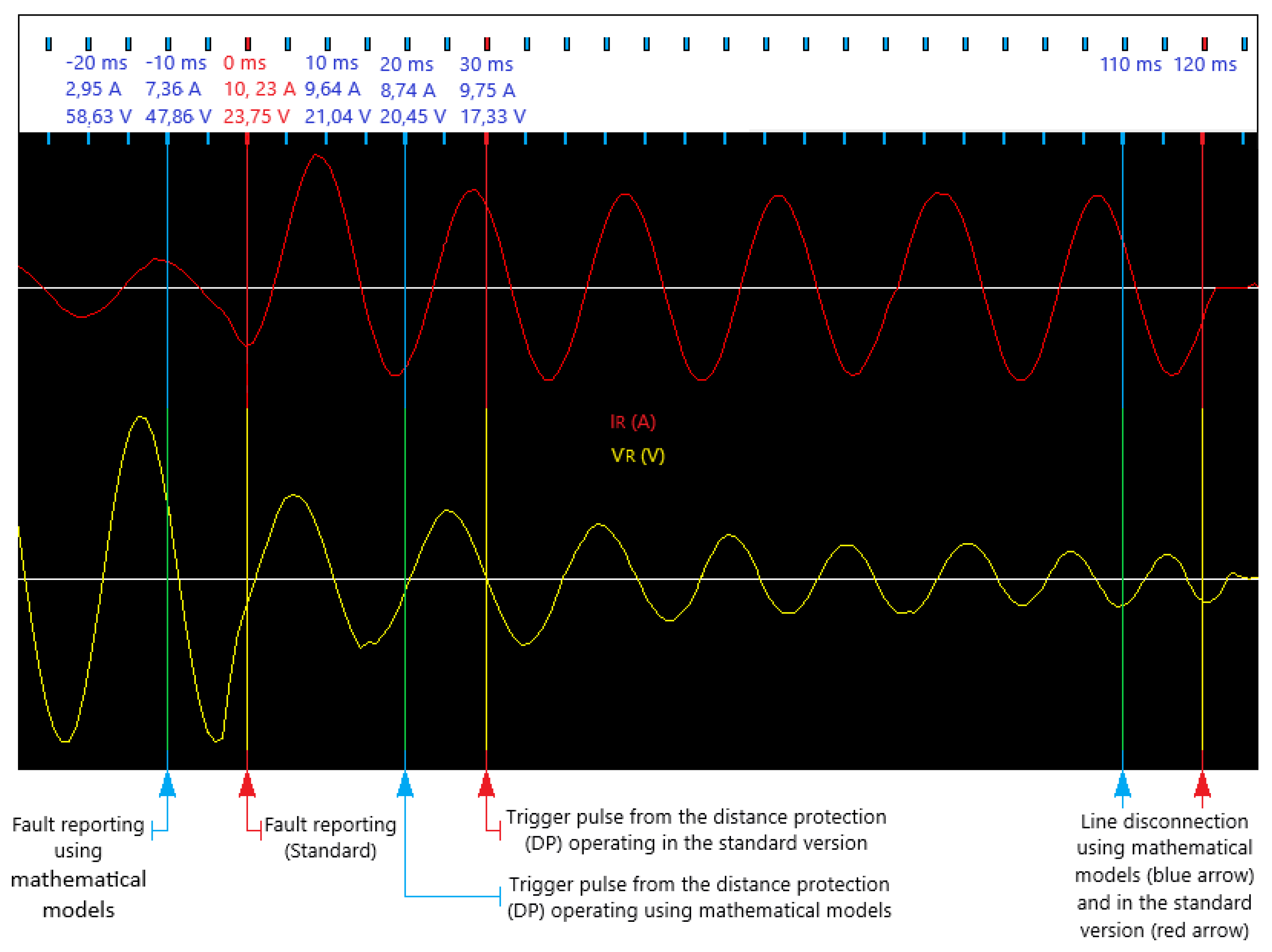
The mathematical models obtained allowed the design of a structure for rapid identification of the occurrence of the fault and triggering of the protection relay. If two consecutive increases in the error between the effective working value and the instantaneous effective value of the voltage are observed and at the same time two consecutive decreases in the error between the effective working value and the instantaneous effective value of the current are present, the derivative of the voltage signal with respect to time is computed using Euler’s approximation and its minimum value is determined, which represents the novelty aspect of the paper. In conclusion, the highest probability is that the defect will be identified by the proposed solution after 11–12 ms from its initial appearance and 10 ms earlier than the standard operating version, emphasizing the benefits of using our developed control structure for rapid identification of a fault and triggering of the line protection relay. These values make it possible to identify the type of defect (transient/temporary or persistent/permanent) from early stages, also illustrated in
Figure 27.
In standard operation mode, the distance protection triggers either to increase the current or, more often, to decrease the impedance, which is measured by monitoring both voltage and current. These are preset, non-adaptive values, that have to be higher than the minimum fault values to make up for voltage drops and overloads in order to ensure selectivity. Protection timing ensures an actuation in time samples for the selectivity of the triggers to which a directing element also contributes. The execution of the tripping command is ensured by the triggering of the protection relay, conditioned by blocking and automation systems. The operation of distance protection is greatly improved by using mathematical models since it turns into an adaptive protection, no longer dependent on strict, preset values, which allows for faster identification of the appearance of a fault, without jeopardizing its selectivity as shown above.
The proposed solution for rapid fault detection meets all the important requirements needed for a high-performance automatic protection system, namely: safety in operation, speed, selectivity, and sensitivity. Moreover, our solution does not require complex solutions in order to be implemented. The use of the proposed structure creates the possibility of sensitizing the protection for an improved time response, highlighted in
Figure 27, resulting in reduced exposure of installations to high fault currents, avoidance of damage to power lines at the fault location, and avoidance of additional interruptions in the electricity distribution system, due to the avoidance of fault generalization, particularly high short-circuit currents and healthy phase overvoltages.
In conclusion, the fault is detected in the early stage of its manifestation, using the proposed procedure for rapid identification of the appearance of the fault based on mathematical models, developed in this manuscript, and the notification of the defect coincides with the start of the protection and takes place after 11 ms, from the start of the procedure, with the registration of the first consecutive manifestations of the defect, when it is barely perceptible, and 10 ms earlier than the standard operating version, a fact also illustrated in
Figure 27. The advantage of 10 ms is preserved until the line is disconnected by distance protection.
The main advantage of introducing the procedure for quickly identifying the occurrence of a fault respectively for controlling the protection relay by using mathematical models, developed based on real events, consists of high-speed transmission line protection while ensuring power system damage avoidance and minimized system disturbance (thus, proving a more reliable control and actual increase in protection speed).
Using the proposed structure creates the possibility of sensitizing the protections for a much-improved response time, highlighted in
Figure 27, resulting in lower disconnected fault currents, the avoidance of additional damage to power lines at the fault location, and the avoidance of additional disruptions in the power distribution system.
In addition, in
Section 5 of the manuscript, the viability of applying artificial intelligence methods for fault management applications is proven.


 ,
, 


