
Modified Frequency Regulator Based on TIλ-TDμFF Controller for Interconnected Microgrids with Incorporating Hybrid Renewable Energy Sources

 ,
,  , , , and
Abstract
:1. Introduction
1.1. General Overview
1.2. Literature Review
1.3. Article Contributions
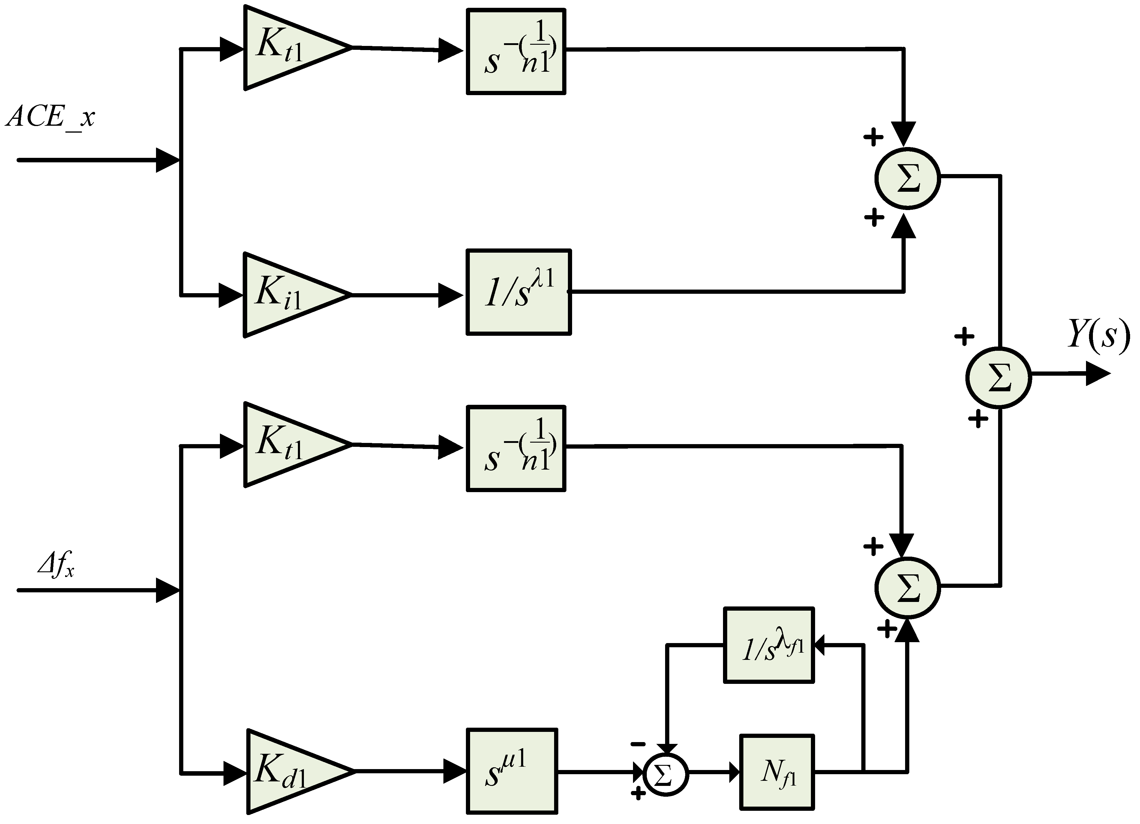
- An improved version of the FO control technique is proposed based on the modified tilt fractional order (FO) integral-tilt FO derivative with fractional filter (TFOI-TFODFF or namely TI-TDFF) controller. The proposed TFOI-TFODFF controller merges the benefits of several FO control capabilities, such as the tilt, FO integral, FO derivative, and FO filter. Thence, the proposed TFOI-TFODFF controller is capable of reducing peak overshoot/undershoot transients and steady-state error compared to existing LFC techniques.
- The proposed TFOI-TFODFF controller employs two control loops compared to some single-loop-based LFC structure. As a consequence, the proposed TFOI-TFODFF controller is capable of mitigating low-frequency as well as high-frequency disturbances in power grids.
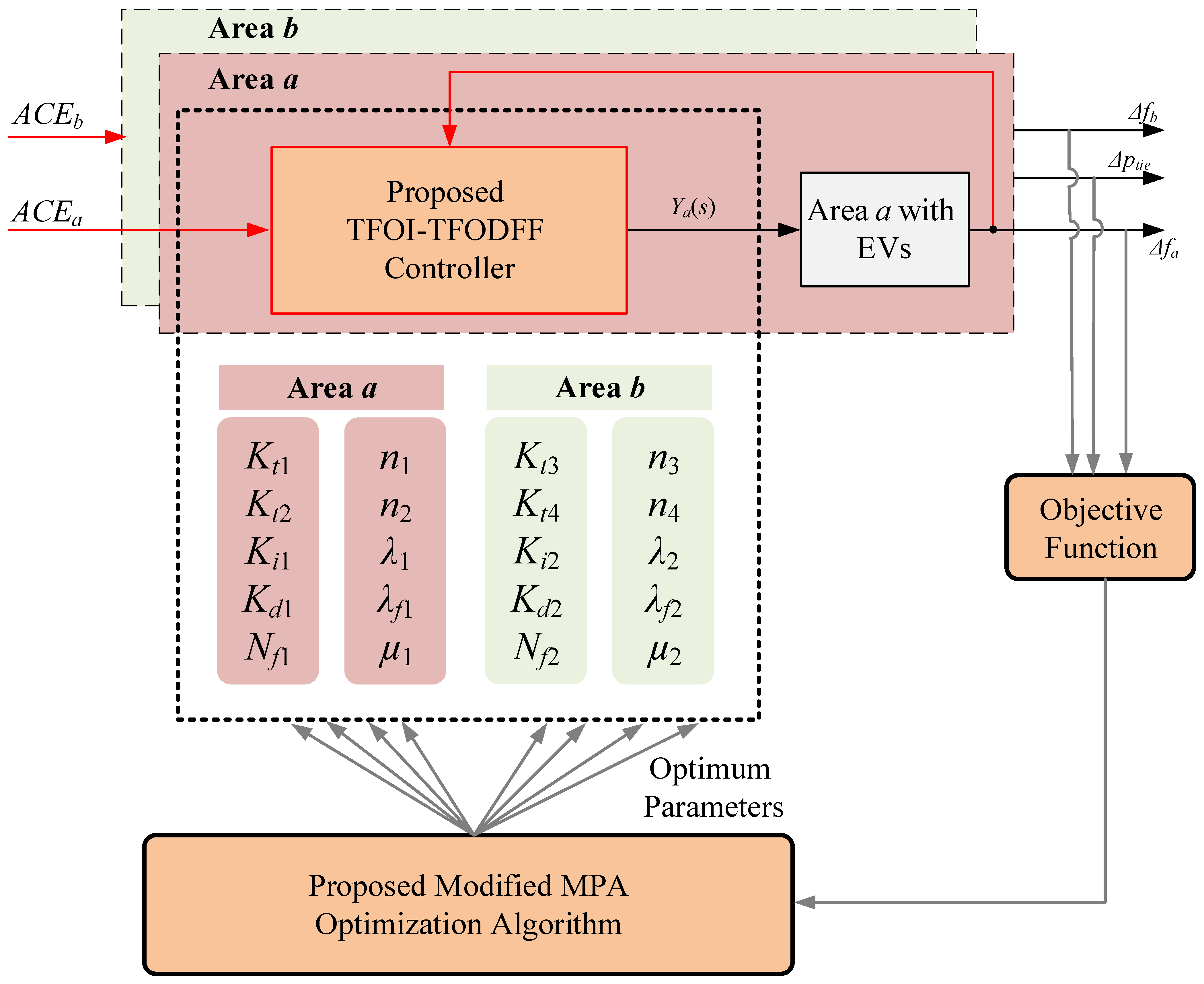
- A coordinated participation of EVs with existing generation power plants is proposed through the proposed TFOI-TFODFF centralized controller. Therefore, EVs can participate effectively in damping systems’ disturbances and fluctuations thanks to their inherent batteries. This can lead to the better utilization of a future high number of connected EVs in power grids.
- A new modified marine predator algorithm (MMPA) is proposed for optimally tuning the controller’s parameters in the proposed TFOI-TFODFF LFC method. The proposed MMPA is modified using a chaotic map and weighting factors to boost the performance of the MMPA. The employed chaotic map can generate a high diverse-based initial population, whereas the weighting factor enhances the exploitation capabilities of the algorithm and accelerates the convergence in the subsequent iterations. The MMPA algorithm is being adopted for tuning the optimal parameters in the new proposed TFOI-TFODFF LFC method.
- A comprehensive statistical analysis is being performed to investigate the effectiveness of the MMPA using parametric and nonparametric tests.
2. Mathematical Representations of Selected Power Grid
2.1. System Construction
2.2. Mathematical Models
3. Proposed TFOI-TFODFF Controller
4. Proposed Modified MPA Optimizer
4.1. Marine Predators Algorithm
4.1.1. High Velocity Ratio
4.1.2. Unit Velocity Ratio
4.1.3. Low Velocity Ratio
| Algorithm 1 Pseudocode of MPA. |
|
4.2. Modified MPA
| Algorithm 2 Pseudocode of WCMPA. |
|
5. Optimizer Verification Results
5.1. Parametric Test
5.2. Nonparametric Test
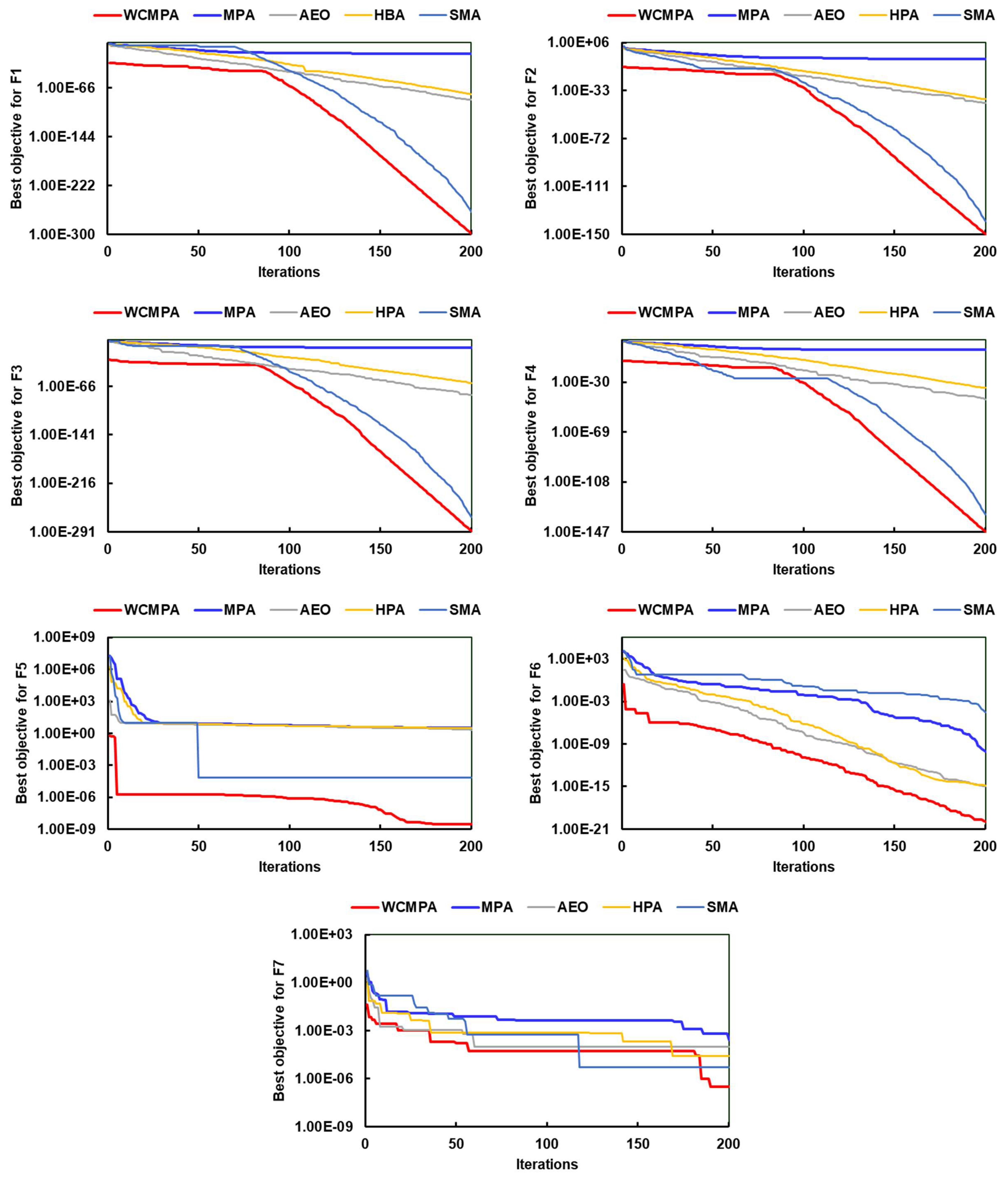
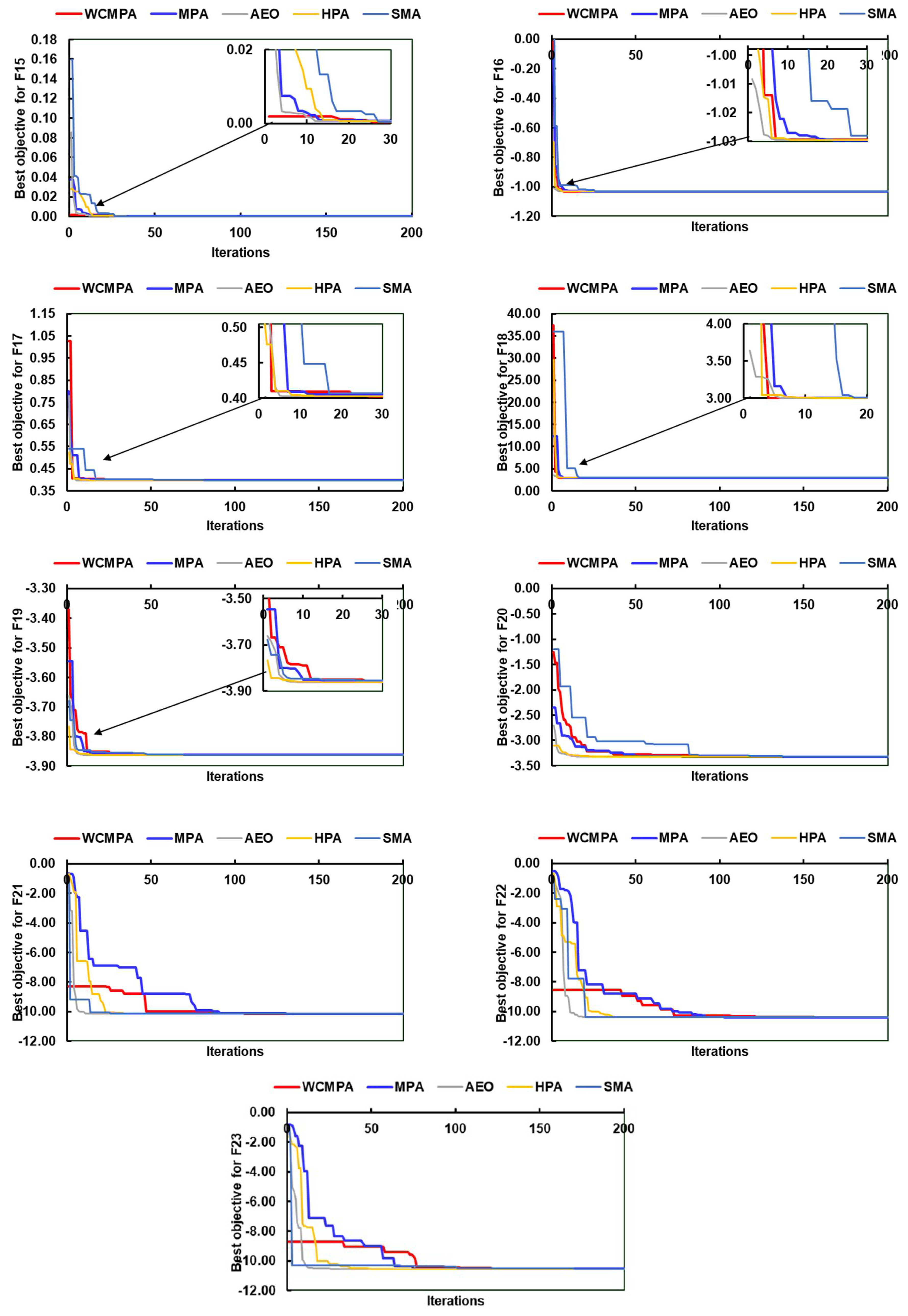
5.3. MMPA Convergence Characteristics
6. Proposed TFOI-TFODFF LFC Verification Results
- Scenario 1: Applying a 1% step load disturbance (SLD);
- Scenario 2: Applying 10% multi-step disturbances (MSD);
- Scenario 3: Applying a random load profile (RLP);
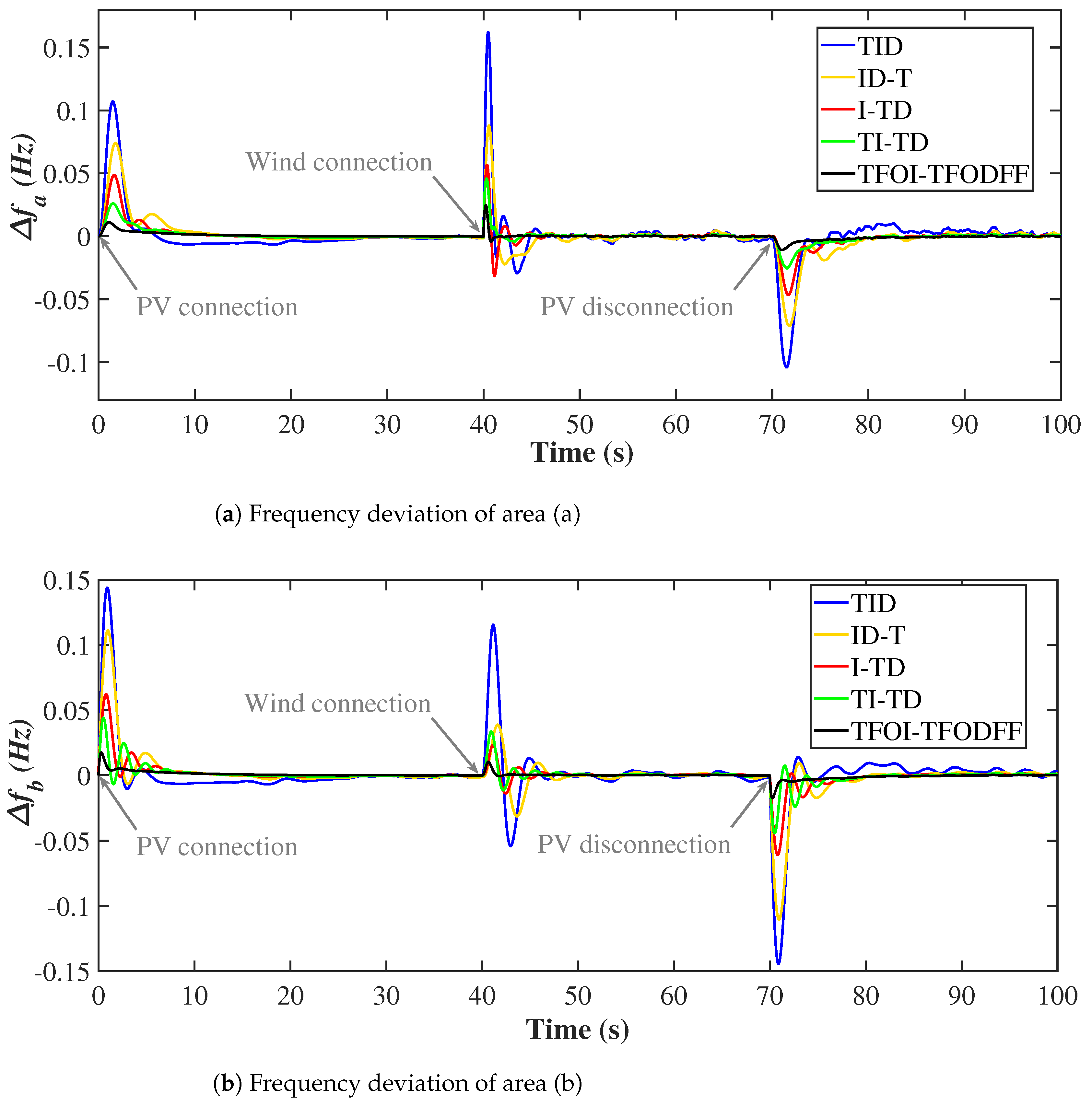
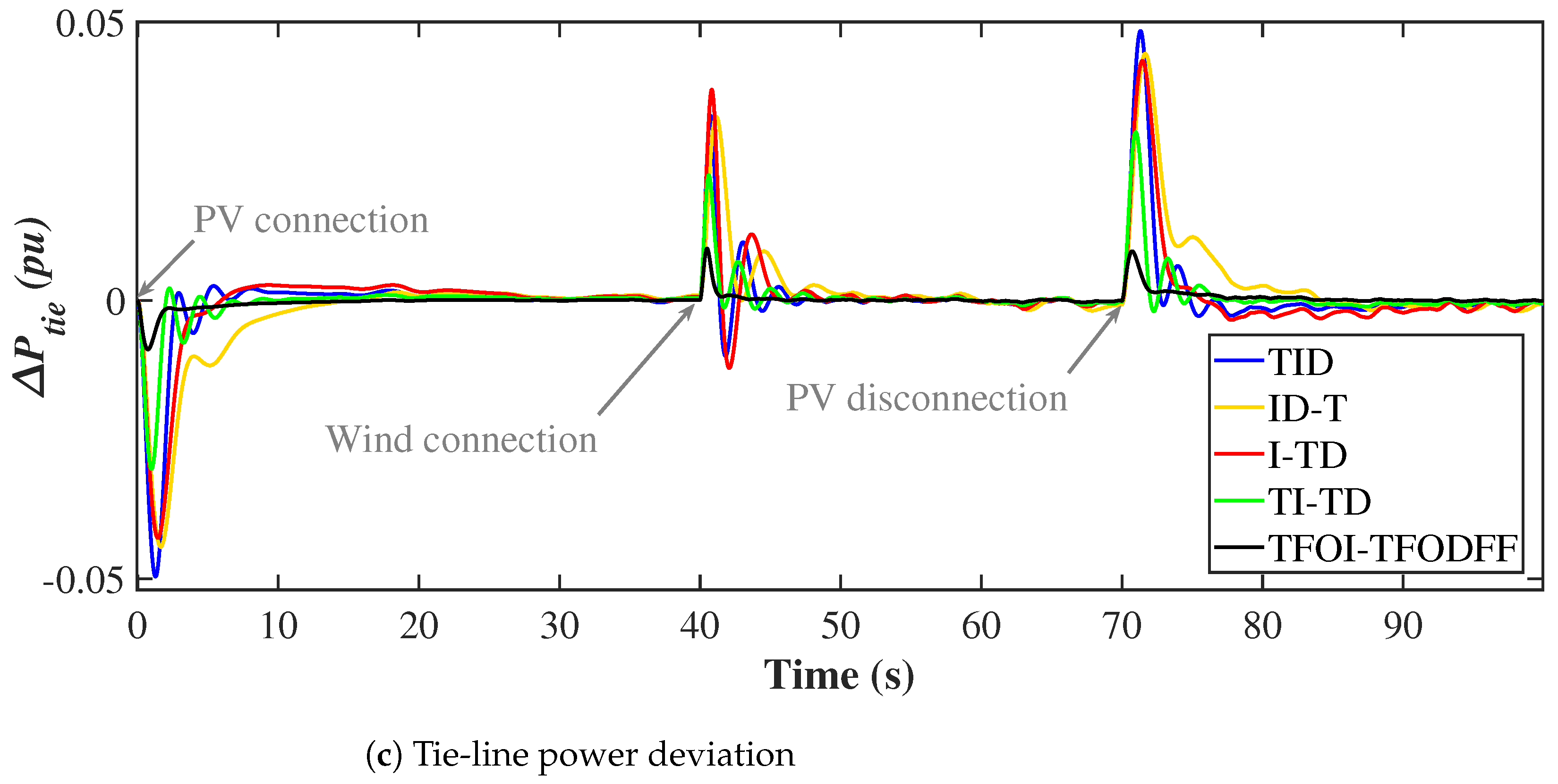
- Scenario 4: Applying a variation of RESs;
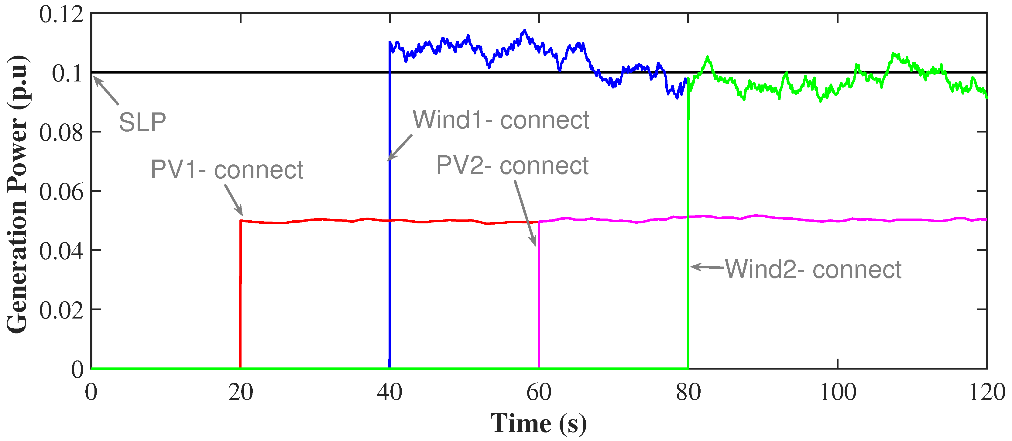
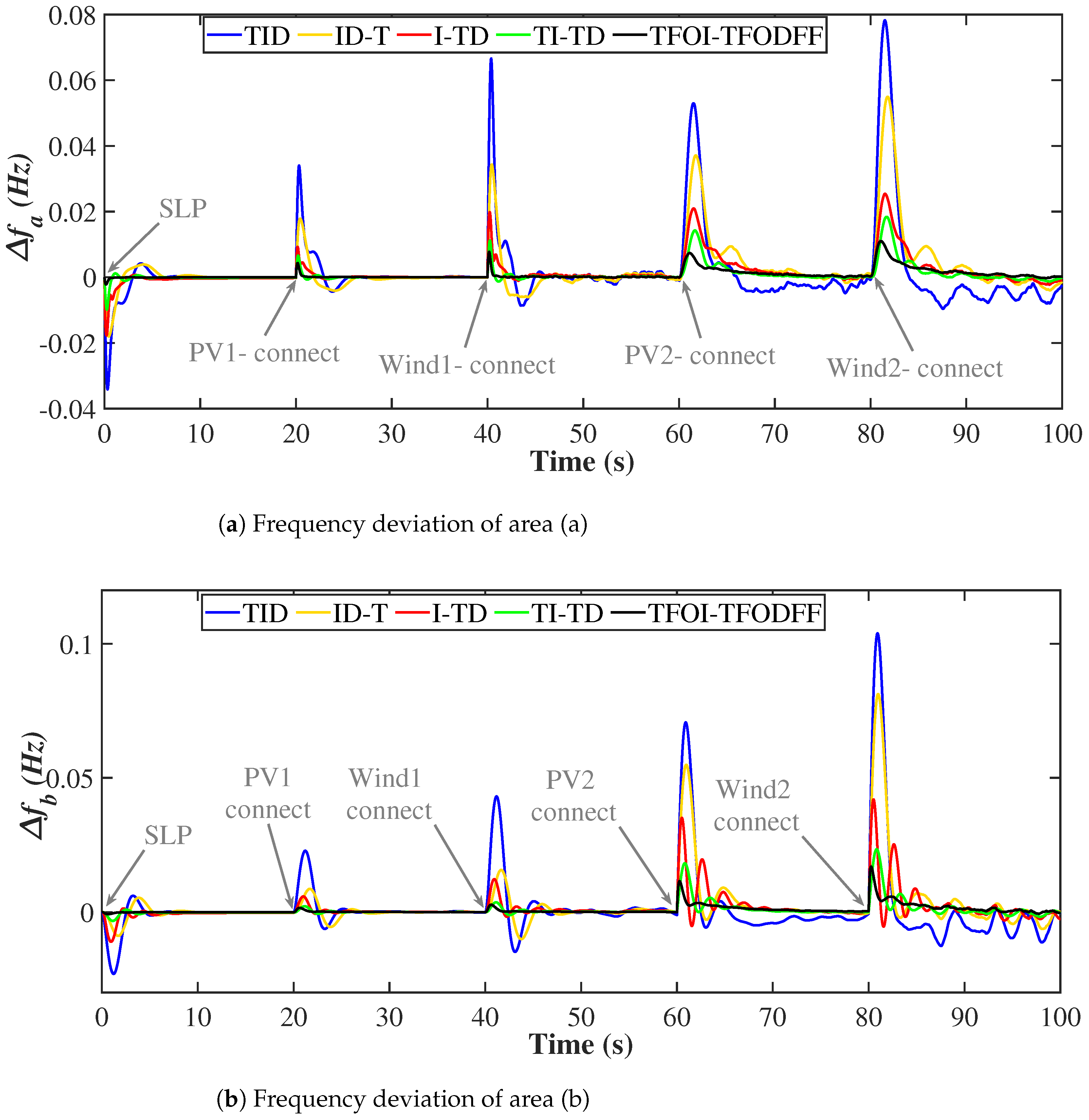
- Scenario 5: Applying a high penetration of RESs.
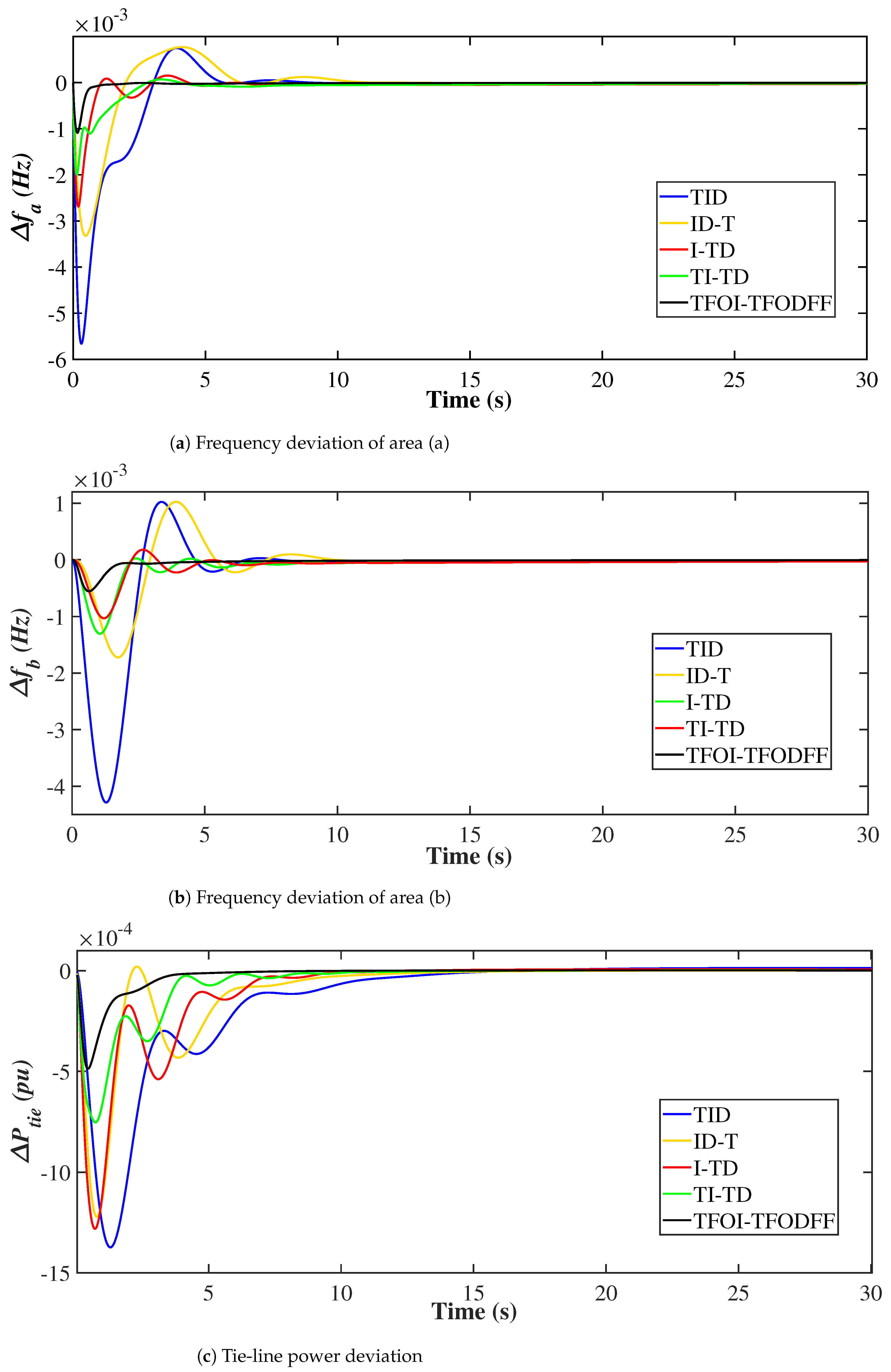
6.1. Scenario 1
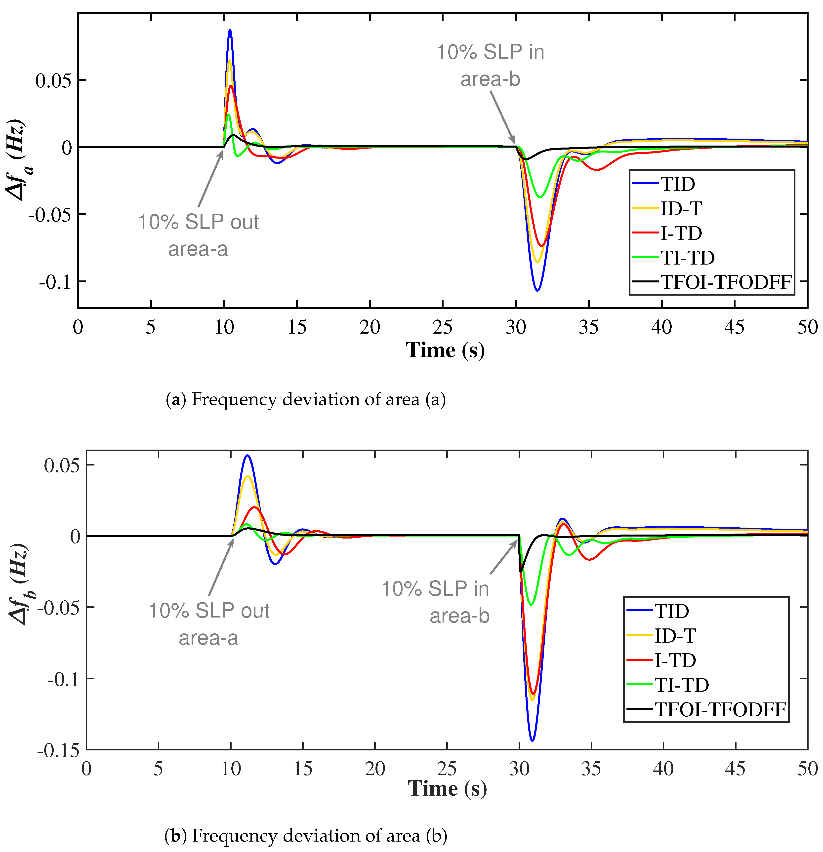
6.2. Scenario 2
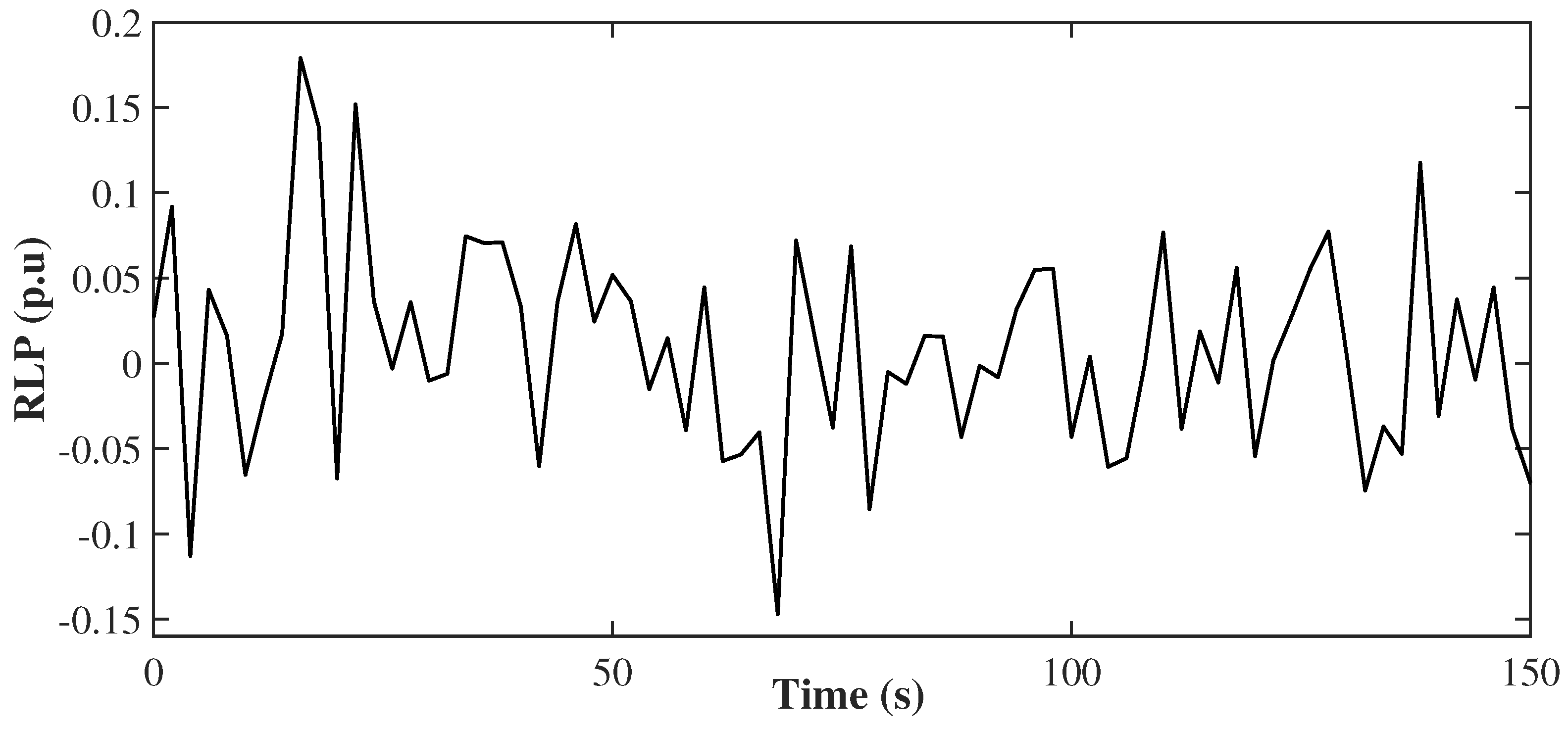
6.3. Scenario 3
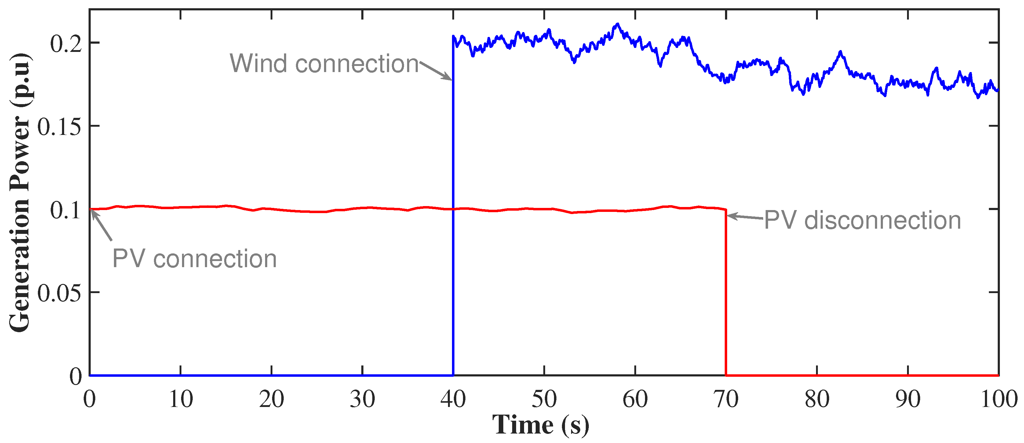
6.4. Scenario 4
6.5. Scenario 5
7. Conclusions
Author Contributions
Funding
Institutional Review Board Statement
Informed Consent Statement
Data Availability Statement
Conflicts of Interest
References
- Ranjan, M.; Shankar, R. A literature survey on load frequency control considering renewable energy integration in power system: Recent trends and future prospects. J. Energy Storage 2022, 45, 103717. [Google Scholar] [CrossRef]
- Bakhtadze, N.; Maximov, E.; Maximova, N. Digital Identification Algorithms for Primary Frequency Control in Unified Power System. Mathematics 2021, 9, 2875. [Google Scholar] [CrossRef]
- Dreidy, M.; Mokhlis, H.; Mekhilef, S. Inertia response and frequency control techniques for renewable energy sources: A review. Renew. Sustain. Energy Rev. 2017, 69, 144–155. [Google Scholar] [CrossRef]
- Shankar, R.; Pradhan, S.; Chatterjee, K.; Mandal, R. A comprehensive state of the art literature survey on LFC mechanism for power system. Renew. Sustain. Energy Rev. 2017, 76, 1185–1207. [Google Scholar] [CrossRef]
- Khamies, M.; Magdy, G.; Ebeed, M.; Kamel, S. A robust PID controller based on linear quadratic gaussian approach for improving frequency stability of power systems considering renewables. ISA Trans. 2021, 117, 118–138. [Google Scholar] [CrossRef]
- Fernández-Guillamón, A.; Gómez-Lázaro, E.; Muljadi, E.; Molina-García, Á. Power systems with high renewable energy sources: A review of inertia and frequency control strategies over time. Renew. Sustain. Energy Rev. 2019, 115, 109369. [Google Scholar] [CrossRef] [Green Version]
- Pandey, S.K.; Mohanty, S.R.; Kishor, N. A literature survey on load–frequency control for conventional and distribution generation power systems. Renew. Sustain. Energy Rev. 2013, 25, 318–334. [Google Scholar] [CrossRef]
- Rakhshani, E.; Rodriguez, P.; Cantarellas, A.M.; Remon, D. Analysis of derivative control based virtual inertia in multi-area high-voltage direct current interconnected power systems. IET Gener. Transm. Distrib. 2016, 10, 1458–1469. [Google Scholar] [CrossRef] [Green Version]
- Kerdphol, T.; Rahman, F.S.; Mitani, Y.; Watanabe, M.; Kufeoglu, S. Robust Virtual Inertia Control of an Islanded Microgrid Considering High Penetration of Renewable Energy. IEEE Access 2018, 6, 625–636. [Google Scholar] [CrossRef]
- Lv, X.; Sun, Y.; Wang, Y.; Dinavahi, V. Adaptive Event-Triggered Load Frequency Control of Multi-Area Power Systems Under Networked Environment via Sliding Mode Control. IEEE Access 2020, 8, 86585–86594. [Google Scholar] [CrossRef]
- Vrdoljak, K.; Perić, N.; Petrović, I. Sliding mode based load-frequency control in power systems. Electr. Power Syst. Res. 2010, 80, 514–527. [Google Scholar] [CrossRef]
- Pan, C.; Liaw, C. An adaptive controller for power system load-frequency control. IEEE Trans. Power Syst. 1989, 4, 122–128. [Google Scholar] [CrossRef]
- Kocaarslan, İ.; Çam, E. Fuzzy logic controller in interconnected electrical power systems for load-frequency control. Int. J. Electr. Power Energy Syst. 2005, 27, 542–549. [Google Scholar] [CrossRef]
- Bu, X.; Yu, W.; Cui, L.; Hou, Z.; Chen, Z. Event-Triggered Data-Driven Load Frequency Control for Multiarea Power Systems. IEEE Trans. Ind. Informatics 2022, 18, 5982–5991. [Google Scholar] [CrossRef]
- Khokhar, B.; Dahiya, S.; Singh Parmar, K.P. Atom search optimization based study of frequency deviation response of a hybrid power system. In Proceedings of the 2020 IEEE 9th Power India International Conference (PIICON), Sonepat, India, 28 February–1 March 2020; pp. 1–5. [Google Scholar] [CrossRef]
- Panda, S.; Mohanty, B.; Hota, P. Hybrid BFOA-PSO algorithm for automatic generation control of linear and nonlinear interconnected power systems. Appl. Soft Comput. 2013, 13, 4718–4730. [Google Scholar] [CrossRef]
- Gupta, D.K.; Soni, A.K.; Jha, A.V.; Mishra, S.K.; Appasani, B.; Srinivasulu, A.; Bizon, N.; Thounthong, P. Hybrid Gravitational–Firefly Algorithm-Based Load Frequency Control for Hydrothermal Two-Area System. Mathematics 2021, 9, 712. [Google Scholar] [CrossRef]
- Arora, K.; Kumar, A.; Kamboj, V.K.; Prashar, D.; Shrestha, B.; Joshi, G.P. Impact of Renewable Energy Sources into Multi Area Multi-Source Load Frequency Control of Interrelated Power System. Mathematics 2021, 9, 186. [Google Scholar] [CrossRef]
- Kumar, A.; Gupta, D.K.; Ghatak, S.R.; Appasani, B.; Bizon, N.; Thounthong, P. A Novel Improved GSA-BPSO Driven PID Controller for Load Frequency Control of Multi-Source Deregulated Power System. Mathematics 2022, 10, 3255. [Google Scholar] [CrossRef]
- Delassi, A.; Arif, S.; Mokrani, L. Load frequency control problem in interconnected power systems using robust fractional PI λ D controller. Ain Shams Eng. J. 2018, 9, 77–88. [Google Scholar] [CrossRef]
- Yousri, D.; Babu, T.S.; Fathy, A. Recent methodology based Harris Hawks optimizer for designing load frequency control incorporated in multi-interconnected renewable energy plants. Sustain. Energy Grids Netw. 2020, 22, 100352. [Google Scholar] [CrossRef]
- Salama, H.S.; Magdy, G.; Bakeer, A.; Vokony, I. Adaptive coordination control strategy of renewable energy sources, hydrogen production unit, and fuel cell for frequency regulation of a hybrid distributed power system. Prot. Control Mod. Power Syst. 2022, 7. [Google Scholar] [CrossRef]
- El Yakine Kouba, N.; Menaa, M.; Hasni, M.; Boudour, M. Optimal load frequency control based on artificial bee colony optimization applied to single, two and multi-area interconnected power systems. In Proceedings of the 2015 3rd International Conference on Control, Engineering & Information Technology (CEIT), Tlemcen, Algeria, 25–27 May 2015; pp. 1–6. [Google Scholar] [CrossRef]
- Sharma, J.; Hote, Y.V.; Prasad, R. PID controller design for interval load frequency control system with communication time delay. Control Eng. Pract. 2019, 89, 154–168. [Google Scholar] [CrossRef]
- Dahab, Y.A.; Abubakr, H.; Mohamed, T.H. Adaptive Load Frequency Control of Power Systems Using Electro-Search Optimization Supported by the Balloon Effect. IEEE Access 2020, 8, 7408–7422. [Google Scholar] [CrossRef]
- Fathy, A.; Alharbi, A.G. Recent Approach Based Movable Damped Wave Algorithm for Designing Fractional-Order PID Load Frequency Control Installed in Multi-Interconnected Plants With Renewable Energy. IEEE Access 2021, 9, 71072–71089. [Google Scholar] [CrossRef]
- Ayas, M.S.; Sahin, E. FOPID controller with fractional filter for an automatic voltage regulator. Comput. Electr. Eng. 2021, 90, 106895. [Google Scholar] [CrossRef]
- Oshnoei, S.; Oshnoei, A.; Mosallanejad, A.; Haghjoo, F. Contribution of GCSC to regulate the frequency in multi-area power systems considering time delays: A new control outline based on fractional order controllers. Int. J. Electr. Power Energy Syst. 2020, 123, 106197. [Google Scholar] [CrossRef]
- Oshnoei, A.; Khezri, R.; Muyeen, S.M.; Oshnoei, S.; Blaabjerg, F. Automatic Generation Control Incorporating Electric Vehicles. Electr. Power Components Syst. 2019, 47, 720–732. [Google Scholar] [CrossRef]
- Priyadarshani, S.; Subhashini, K.R.; Satapathy, J.K. Pathfinder algorithm optimized fractional order tilt-integral-derivative (FOTID) controller for automatic generation control of multi-source power system. Microsyst. Technol. 2021, 27, 23–35. [Google Scholar] [CrossRef]
- Sahu, R.K.; Panda, S.; Biswal, A.; Sekhar, G.C. Design and analysis of tilt integral derivative controller with filter for load frequency control of multi-area interconnected power systems. ISA Trans. 2016, 61, 251–264. [Google Scholar] [CrossRef]
- Elkasem, A.H.A.; Kamel, S.; Hassan, M.H.; Khamies, M.; Ahmed, E.M. An Eagle Strategy Arithmetic Optimization Algorithm for Frequency Stability Enhancement Considering High Renewable Power Penetration and Time-Varying Load. Mathematics 2022, 10, 854. [Google Scholar] [CrossRef]
- Ahmed, E.M.; Mohamed, E.A.; Elmelegi, A.; Aly, M.; Elbaksawi, O. Optimum Modified Fractional Order Controller for Future Electric Vehicles and Renewable Energy-Based Interconnected Power Systems. IEEE Access 2021, 9, 29993–30010. [Google Scholar] [CrossRef]
- Mohamed, E.A.; Aly, M.; Watanabe, M. New Tilt Fractional-Order Integral Derivative with Fractional Filter (TFOIDFF) Controller with Artificial Hummingbird Optimizer for LFC in Renewable Energy Power Grids. Mathematics 2022, 10, 3006. [Google Scholar] [CrossRef]
- Arya, Y. A novel CFFOPI-FOPID controller for AGC performance enhancement of single and multi-area electric power systems. ISA Trans. 2020, 100, 126–135. [Google Scholar] [CrossRef]
- Arya, Y.; Kumar, N.; Dahiya, P.; Sharma, G.; Çelik, E.; Dhundhara, S.; Sharma, M. Cascade-IλDμN controller design for AGC of thermal and hydro-thermal power systems integrated with renewable energy sources. IET Renew. Power Gener. 2021. [Google Scholar] [CrossRef]
- Arya, Y. A new optimized fuzzy FOPI-FOPD controller for automatic generation control of electric power systems. J. Frankl. Inst. 2019, 356, 5611–5629. [Google Scholar] [CrossRef]
- Gheisarnejad, M.; Khooban, M.H. Design an optimal fuzzy fractional proportional integral derivative controller with derivative filter for load frequency control in power systems. Trans. Inst. Meas. Control 2019, 41, 2563–2581. [Google Scholar] [CrossRef]
- Arya, Y. Improvement in automatic generation control of two-area electric power systems via a new fuzzy aided optimal PIDN-FOI controller. ISA Trans. 2018, 80, 475–490. [Google Scholar] [CrossRef]
- Latif, A.; Hussain, S.M.S.; Das, D.C.; Ustun, T.S. Optimum Synthesis of a BOA Optimized Novel Dual-Stage PI - (1 + ID) Controller for Frequency Response of a Microgrid. Energies 2020, 13, 3446. [Google Scholar] [CrossRef]
- Malik, S.; Suhag, S. A Novel SSA Tuned PI-TDF Control Scheme for Mitigation of Frequency Excursions in Hybrid Power System. Smart Sci. 2020, 8, 202–218. [Google Scholar] [CrossRef]
- Shiva, C.; Shankar, G.; Mukherjee, V. Automatic generation control of power system using a novel quasi-oppositional harmony search algorithm. Int. J. Electr. Power Energy Syst. 2015, 73, 787–804. [Google Scholar] [CrossRef]
- Mohanty, B.; Panda, S.; Hota, P.K. Controller parameters tuning of differential evolution algorithm and its application to load frequency control of multi-source power system. Int. J. Electr. Power Energy Syst. 2014, 54, 77–85. [Google Scholar] [CrossRef]
- Sahu, R.; Panda, S.; Rout, U.K.; Sahoo, D. Teaching learning based optimization algorithm for automatic generation control of power system using 2-DOF PID controller. Int. J. Electr. Power Energy Syst. 2016, 77, 287–301. [Google Scholar] [CrossRef]
- Dash, P.; Saikia, L.; Sinha, N. Automatic generation control of multi area thermal system using Bat algorithm optimized PD–PID cascade controller. Int. J. Electr. Power Energy Syst. 2015, 68, 364–372. [Google Scholar] [CrossRef]
- Raju, M.; Saikia, L.; Sinha, N. Automatic generation control of a multi-area system using ant lion optimizer algorithm based PID plus second order derivative controller. Int. J. Electr. Power Energy Syst. 2016, 80, 52–63. [Google Scholar] [CrossRef]
- Gheisarnejad, M. An effective hybrid harmony search and cuckoo optimization algorithm based fuzzy PID controller for load frequency control. Appl. Soft Comput. 2018, 65, 121–138. [Google Scholar] [CrossRef]
- Prakash, S.; Sinha, S. Simulation based neuro-fuzzy hybrid intelligent PI control approach in four-area load frequency control of interconnected power system. Appl. Soft Comput. 2014, 23, 152–164. [Google Scholar] [CrossRef]
- Latif, A.; Paul, M.; Das, D.C.; Hussain, S.M.S.; Ustun, T.S. Price Based Demand Response for Optimal Frequency Stabilization in ORC Solar Thermal Based Isolated Hybrid Microgrid under Salp Swarm Technique. Electronics 2020, 9, 2209. [Google Scholar] [CrossRef]
- Hussain, I.; Das, D.C.; Latif, A.; Sinha, N.; Hussain, S.S.; Ustun, T.S. Active power control of autonomous hybrid power system using two degree of freedom PID controller. Energy Rep. 2022, 8, 973–981. [Google Scholar] [CrossRef]
- Mohamed, E.A.; Ahmed, E.M.; Elmelegi, A.; Aly, M.; Elbaksawi, O.; Mohamed, A.A.A. An Optimized Hybrid Fractional Order Controller for Frequency Regulation in Multi-area Power Systems. IEEE Access 2020, 8, 213899–213915. [Google Scholar] [CrossRef]
- Abraham, R.J.; Das, D.; Patra, A. Automatic generation control of an interconnected hydrothermal power system considering superconducting magnetic energy storage. Int. J. Electr. Power Energy Syst. 2007, 29, 571–579. [Google Scholar] [CrossRef]
- Singh, K.; Amir, M.; Ahmad, F.; Khan, M.A. An Integral Tilt Derivative Control Strategy for Frequency Control in Multimicrogrid System. IEEE Syst. J. 2021, 15, 1477–1488. [Google Scholar] [CrossRef]
- Kumari, S.; Shankar, G. Novel application of integral-tilt-derivative controller for performance evaluation of load frequency control of interconnected power system. IET Gener. Transm. Distrib. 2018, 12, 3550–3560. [Google Scholar] [CrossRef]
- Ahmed, M.; Magdy, G.; Khamies, M.; Kamel, S. Modified TID controller for load frequency control of a two-area interconnected diverse-unit power system. Int. J. Electr. Power Energy Syst. 2022, 135, 107528. [Google Scholar] [CrossRef]


| Parameters | Symbols | Value | |
|---|---|---|---|
| Area a | Area b | ||
| Rated capacities | (MW) | 1200 | 1200 |
| Droop constants | (Hz/MW) | 2.4 | 2.4 |
| Frequency biases | (MW/Hz) | 0.4249 | 0.4249 |
| Valve gate limit (minimum) | (p.u.MW) | −0.5 | −0.5 |
| Valve gate limit (maximum) | (p.u.MW) | 0.5 | 0.5 |
| Time constant of thermal governor | (s) | 0.08 | - |
| Thermal turbines (time constants) | (s) | 0.3 | - |
| Hydraulic governor (time constants) | (s) | - | 41.6 |
| Transient droop for hydraulic governor (time constants) | (s) | - | 0.513 |
| Hydraulic governor (reset times) | (s) | - | 5 |
| Hydro turbine (water starting times) | (s) | - | 1 |
| Inertia constants | (p.u.s) | 0.0833 | 0.0833 |
| Damping coefficients | (p.u./Hz) | 0.00833 | 0.00833 |
| PV generation (time constants) | (s) | - | 1.3 |
| PV generation (gains) | (s) | - | 1 |
| Wind generation (time constants) | (s) | 1.5 | - |
| Wind generation (gains) | (s) | 1 | - |
| EV models | |||
| Penetrations level | - | 5–10% | 5–10% |
| Voltages (nominal value) | (V) | 364.8 | 364.8 |
| Batteries capacities | (Ah) | 66.2 | 66.2 |
| Series resistance | (ohms) | 0.074 | 0.074 |
| Transient resistance | (ohms) | 0.047 | 0.047 |
| Transient capacitance | (farad) | 703.6 | 703.6 |
| Constant values | 0.02612 | 0.02612 | |
| Battery’s SOC (maximum limits) | % | 95 | 95 |
| Battery’s energy capacities | (kWh) | 24.15 | 24.15 |
| WCMPA | MPA | AEO | HPA | SMA | ||
|---|---|---|---|---|---|---|
| F1 | Best | 5.33 × 10 | 4.23 × | 1.06 × | 7.14 × 10 | 2.02 × |
| Average | 2.47 × | 5.86 × | 5.89 × | 1.49 × | 2.91 × | |
| Worst | 6.80 × | 2.61 × | 1.76 × | 3.00 × | 8.74 × | |
| F2 | Best | 2.24 × | 7.91 × | 7.16 × | 9.27 × | 5.89 × |
| Average | 7.06 × | 7.33 × | 5.17 × | 2.97 × | 3.14 × | |
| Worst | 1.29 × | 2.05 × | 6.05 × | 4.00 × | 9.42 × | |
| F3 | Best | 2.10 × | 1.49 × | 7.09 × | 1.35 × | 5.30 × |
| Average | 1.01 × | 8.96 × | 4.57 × | 9.37 × | 4.59 × | |
| Worst | 2.16 × | 4.44 × | 1.36 × | 2.23 × | 8.37 × | |
| F4 | Best | 1.60 × | 2.94 × | 2.33 × | 2.97 × | 2.29 × |
| Average | 8.53 × | 8.69 × | 3.81 × | 2.99 × | 4.43 × | |
| Worst | 6.90 × | 2.23 × | 1.03 × | 4.72 × | 1.04 × | |
| F5 | Best | 2.83 × | 3.37 × | 2.14 × | 3.01 × | 6.85 × |
| Average | 2.47 × | 4.49 × | 3.12 × | 3.56 × | 2.39 × | |
| Worst | 1.33 × | 5.81 × | 4.66 × | 4.33 × | 7.42 × | |
| F6 | Best | 1.05 × | 9.38 × | 1.01 × | 1.52 × | 3.21 × |
| Average | 4.78 × | 2.50 × | 5.53 × | 2.66 × | 1.20 × | |
| Worst | 2.26 × | 8.01 × | 6.03 × | 5.66 × | 2.66 × | |
| F7 | Best | 3.05 × | 2.86 × | 1.01 × | 2.59 × | 5.23 × |
| Average | 5.87 × | 1.67 × | 8.67 × | 4.13 × | 1.84 × | |
| Worst | 1.58 × | 4.91 × | 2.94 × | 1.34 × | 6.16 × |
| WCMPA | MPA | AEO | HPA | SMA | ||
|---|---|---|---|---|---|---|
| F8 | Best | −4.19 × | −4.07 × | −4.19 × | −4.07 × | −4.19 × |
| Average | −4.19 × | −3.51 × | −3.88 × | −3.46 × | −4.19 × | |
| Worst | −4.19 × | −3.16 × | −3.48 × | −2.76 × | −4.19 × | |
| F9 | Best | 0.0000 | 0.0000 | 0.0000 | 0.0000 | 0.0000 |
| Average | 0.0000 | 0.0717 | 0.0000 | 0.0000 | 0.0000 | |
| Worst | 0.0000 | 1.0126 | 0.0000 | 0.0000 | 0.0000 | |
| F10 | Best | 8.88 × | 3.64 × | 8.88 × | 8.88 × | 8.88 × |
| Average | 8.88 × | 3.36 × | 8.88 × | 8.88 × | 8.88 × | |
| Worst | 8.88 × | 7.33 × | 8.88 × | 8.88 × | 8.88 × | |
| F11 | Best | 0.00 × | 4.68 × | 0.00 × | 0.00 × | 0.00 × |
| Average | 0.00 × | 1.97 × | 0.00 × | 0.00 × | 0.00 × | |
| Worst | 0.00 × | 4.37 × | 0.00 × | 0.00 × | 0.00 × | |
| F12 | Best | 1.11 × | 1.46 × | 1.49 × | 6.38 × | 1.21 × |
| Average | 3.96 × | 2.28 × | 1.40 × | 1.58 × | 1.89 × | |
| Worst | 4.45 × | 1.00 × | 2.70 × | 1.95 × | 5.30 × | |
| F13 | Best | 1.16 × | 1.30 × | 1.50 × | 1.63 × | 4.30 × |
| Average | 4.61 × | 1.01 × | 1.28 × | 9.06 × | 3.42 × | |
| Worst | 2.33 × | 2.75 × | 1.10 × | 9.74 × | 1.49 × | |
| F14 | Best | 0.99800 | 0.99800 | 0.99800 | 0.99800 | 0.99800 |
| Average | 0.99800 | 0.99800 | 0.99800 | 1.16341 | 0.99800 | |
| Worst | 0.99800 | 0.99800 | 0.99800 | 2.98211 | 0.99800 |
| WCMPA | MPA | AEO | HPA | SMA | ||
|---|---|---|---|---|---|---|
| F15 | Best | 0.00031 | 0.00031 | 0.00031 | 0.00031 | 0.00031 |
| Average | 0.00031 | 0.00031 | 0.00042 | 0.00249 | 0.00066 | |
| Worst | 0.00033 | 0.00033 | 0.00159 | 0.02255 | 0.00125 | |
| F16 | Best | −1.03163 | −1.03163 | −1.03163 | −1.03163 | −1.03163 |
| Average | −1.03163 | −1.03163 | −1.03163 | −1.03163 | −1.03163 | |
| Worst | −1.03163 | −1.03163 | −1.03163 | −1.03163 | −1.03163 | |
| F17 | Best | 0.39789 | 0.39789 | 0.39789 | 0.39789 | 0.39789 |
| Average | 0.39789 | 0.39789 | 0.39789 | 0.39789 | 0.39789 | |
| Worst | 0.39789 | 0.39789 | 0.39789 | 0.39789 | 0.39789 | |
| F18 | Best | 3.00000 | 3.00000 | 3.00000 | 3.00000 | 3.00000 |
| Average | 3.00000 | 3.00000 | 3.00000 | 3.00000 | 3.00000 | |
| Worst | 3.00000 | 3.00000 | 3.00000 | 3.00000 | 3.00000 | |
| F19 | Best | −3.86278 | −3.86278 | −3.86278 | −3.86278 | −3.86278 |
| Average | −3.86278 | −3.86278 | −3.86278 | −3.86226 | −3.86272 | |
| Worst | −3.86278 | −3.86278 | −3.86278 | −3.85490 | −3.86091 | |
| F20 | Best | −3.32194 | −3.32200 | −3.32200 | −3.32200 | −3.32198 |
| Average | −3.32091 | −3.32200 | −3.27840 | −3.25151 | −3.26175 | |
| Worst | −3.31672 | −3.32200 | −3.20310 | −2.84042 | −3.19766 | |
| F21 | Best | −10.15274 | −10.15320 | −10.15320 | −10.15320 | −10.15319 |
| Average | −10.15097 | −10.15320 | −9.15017 | −9.65168 | −10.15240 | |
| Worst | −10.14359 | −10.15320 | −2.63047 | −2.63047 | −10.14966 | |
| F22 | Best | −10.40259 | −10.40294 | −10.40294 | −10.40294 | −10.40291 |
| Average | −10.39883 | −10.40294 | −9.70313 | −9.00332 | −10.40207 | |
| Worst | −10.38432 | −10.40294 | −2.76590 | −2.76590 | −10.39884 | |
| F23 | Best | −10.53613 | −10.53641 | −10.53641 | −10.53641 | −10.53635 |
| Average | −10.52902 | −10.53641 | −10.31304 | −9.81918 | −10.53558 | |
| Worst | −10.50445 | −10.53641 | −3.83543 | −2.42173 | −10.53370 |
| MPA | AEO | HPA | SMA | ||
|---|---|---|---|---|---|
| F1 | 465 | 465 | 465 | 465 | |
| 0 | 0 | 0 | 0 | ||
| p-Value | 1.78 × | 1.78 × | 1.78 × | 1.78 × | |
| F2 | 465 | 465 | 465 | 465 | |
| 0 | 0 | 0 | 0 | ||
| p-Value | 1.78 × | 1.78 × | 1.78 × | 1.78 × | |
| F3 | 465 | 465 | 465 | 465 | |
| 0 | 0 | 0 | 0 | ||
| p-Value | 1.78 × | 1.78 × | 1.78 × | 1.78 × | |
| F4 | 465 | 465 | 465 | 465 | |
| 0 | 0 | 0 | 0 | ||
| p-Value | 1.78 × | 1.78 × | 1.78 × | 1.78 × | |
| F5 | 465 | 465 | 465 | 465 | |
| 0 | 0 | 0 | 0 | ||
| p-Value | 1.78 × | 1.78 × | 1.78 × | 1.78 × | |
| F6 | 465 | 465 | 465 | 465 | |
| 0 | 0 | 0 | 0 | ||
| p-Value | 1.78 × | 1.78 × | 1.78 × | 1.78 × | |
| F7 | 465 | 465 | 453 | 439 | |
| 0 | 0 | −12 | −26 | ||
| p-Value | 1.78 × | 1.78 × | 5.89 × | 2.21 × |
| MPA | AEO | HPA | SMA | ||
|---|---|---|---|---|---|
| F8 | 465 | 465 | 465 | 465 | |
| 0 | 0 | 0 | 0 | ||
| p-Value | 1.78 × | 1.78 × | 1.78 × | 1.78 × | |
| F9 | 465 | ||||
| 0 | |||||
| p-Value | 1.78 × | ||||
| F10 | |||||
| p-Value | |||||
| F11 | 465 | ||||
| 0 | |||||
| p-Value | 1.78 × | ||||
| F12 | 465 | 465 | 465 | 465 | |
| 0 | 0 | 0 | 0 | ||
| p-Value | 1.78 × | 1.78 × | 1.78 × | 1.78 × | |
| F13 | 465 | 465 | 465 | 465 | |
| 0 | 0 | 0 | 0 | ||
| p-Value | 1.78 × | 1.78 × | 1.78 × | 1.78 × | |
| F14 | 0 | 87 | 3 | 0 | |
| −465 | −378 | −462 | −465 | ||
| p-Value | 1.78 × | 0.002812 | 2.41 × | 1.78 × |
| MPA | AEO | HPA | SMA | ||
|---|---|---|---|---|---|
| F15 | 29 | 87 | 192 | 464 | |
| −436 | −378 | −273 | −1 | ||
| p-Value | 2.91 × | 0.002812 | 4.08 × | 1.97 × | |
| F16 | |||||
| p-Value | |||||
| F17 | |||||
| p-Value | |||||
| F18 | |||||
| p-Value | |||||
| F19 | 59 | 465 | |||
| −28 | 0 | ||||
| p-Value | 0.753774 | 1.78 × | |||
| F20 | 0 | 275 | 312 | 345 | |
| −465 | −190 | −153 | −120 | ||
| p-Value | 1.78 × | 3.85 × | 1.03 × | 2.10 × | |
| F21 | 0 | 114 | 59 | 85 | |
| −465 | −351 | −406 | −380 | ||
| p-Value | 1.78 × | 0.015007 | 3.66 × | 2.46 × | |
| F22 | 0 | 87 | 165 | 48 | |
| −465 | −378 | −300 | −417 | ||
| p-Value | 1.78 × | 0.002812 | 1.67 × | 1.51 × | |
| F23 | 0 | 30 | 87 | 23 | |
| −465 | −435 | −378 | −442 | ||
| p-Value | 1.78 × | 3.18 × | 2.81 × | 1.68 × |
| WCMPA | MPA | AEO | HBA | SMA | |
|---|---|---|---|---|---|
| F1 | 1 | 5 | 3 | 4 | 2 |
| F2 | 1 | 5 | 4 | 3 | 2 |
| F3 | 1 | 5 | 3 | 4 | 2 |
| F4 | 1 | 5 | 3 | 4 | 2 |
| F5 | 1 | 5 | 3 | 4 | 2 |
| F6 | 1 | 3 | 2 | 4 | 5 |
| F7 | 1 | 5 | 4 | 3 | 2 |
| F8 | 1 | 4 | 3 | 5 | 2 |
| F9 | 1 | 5 | 2 | 3 | 4 |
| F10 | 1 | 2 | 3 | 4 | 5 |
| F11 | 1 | 5 | 2 | 3 | 4 |
| F12 | 1 | 4 | 2 | 3 | 5 |
| F13 | 1 | 2 | 3 | 5 | 4 |
| F14 | 4 | 1 | 5 | 3 | 2 |
| F15 | 2 | 1 | 3 | 5 | 4 |
| F16 | 1 | 2 | 3 | 4 | 5 |
| F17 | 1 | 2 | 3 | 4 | 5 |
| F18 | 4 | 2 | 1 | 5 | 3 |
| F19 | 2 | 3 | 5 | 1 | 4 |
| F20 | 2 | 1 | 3 | 5 | 4 |
| F21 | 3 | 1 | 5 | 4 | 2 |
| F22 | 3 | 1 | 4 | 5 | 2 |
| F23 | 3 | 1 | 4 | 5 | 2 |
| Mean Rank | 1.6522 | 3.0435 | 3.1739 | 3.9130 | 3.2174 |
| Rank | 1 | 2 | 3 | 5 | 4 |
| Control | Area | Coefficients | |||||||||
|---|---|---|---|---|---|---|---|---|---|---|---|
| TID | Area a | 1.8022 | ― | 1.9561 | 1.8213 | ― | ― | 3.01 | ― | ― | ― |
| Area b | 1.9763 | ― | 1.2044 | 1.3331 | ― | ― | 2.98 | ― | ― | ||
| ID-T | Area a | 1.8184 | ― | 1.5674 | 0.9969 | ― | ― | 4.95 | ― | ― | ― |
| Area b | 1.8909 | ― | 1.1891 | 1.9492 | ― | ― | 4.91 | ― | ― | ||
| I-TD | Area a | 1.8726 | ― | 1.8859 | 1.7689 | ― | ― | 2.65 | ― | ― | ― |
| Area b | 1.1364 | ― | 0.6997 | 0.4305 | ― | ― | 3.66 | ― | ― | ― | |
| TI-TD | Area a | 4.3749 | 4.9837 | 3.1151 | 1.6403 | ― | ― | 4.58 | 4.37 | ― | ― |
| Area b | 0.5839 | 4.7702 | 0.7011 | 3.3158 | ― | ― | 2.01 | 2.62 | ― | ― | |
| Proposed | Area a | 4.8285 | 4.8577 | 4.7162 | 4.6441 | 0.456 | 0.136 | 4.40 | 3.24 | 207 | 0.745 |
| Area b | 2.7803 | 4.4415 | 0.5121 | 4.9637 | 0.641 | 0.788 | 2.81 | 4.01 | 120 | 0.851 | |
| No. | Controller | |||||||||
|---|---|---|---|---|---|---|---|---|---|---|
| PO | PU | ST | PO | PU | ST | PO | PU | ST | ||
| TID | 0.0007 | 0.0057 | 12 | 0.001 | 0.0041 | 13 | 0.0001 | 0.0014 | 19 | |
| ID-T | 0.0008 | 0.0032 | 14 | 0.0011 | 0.0017 | 16 | 0.0001 | 0.0013 | 19 | |
| No.1 | I-TD | 0.0002 | 0.0027 | 19 | 0.0002 | 0.0013 | 17 | 0.00001 | 0.0012 | 16 |
| TI-TD | 0.00007 | 0.0019 | 17 | 0.0001 | 0.0011 | 18 | 0.00002 | 0.0007 | 15 | |
| Proposed | 0 | 0.0011 | 5 | 0 | 0.0005 | 6 | 0 | 0.0004 | 7 | |
| TID | 0.003 | 0.107 | OS | 0.0121 | 0.1438 | OS | 0.0442 | 0.0113 | OS | |
| ID-T | 0.0025 | 0.0856 | OS | 0.0097 | 0.1152 | OS | 0.0427 | 0.002 | OS | |
| No.2 | I-TD | 0.0071 | 0.0738 | 14 | 0.0083 | 0.1108 | 15 | 0.034 | 0.0015 | OS |
| TI-TD | 0.0067 | 0.0375 | 13 | 0.0008 | 0.0485 | 12 | 0.0289 | 0.0013 | OS | |
| Proposed | 0 | 0.009 | 4 | 0.0004 | 0.0251 | 7 | 0.0046 | 0 | 9 | |
| TID | 0.0652 | 0.0616 | OS | 0.0661 | 0.0769 | OS | 0.0179 | 0.0191 | OS | |
| ID-T | 0.0454 | 0.0522 | OS | 0.0322 | 0.0398 | OS | 0.0141 | 0.0122 | OS | |
| No.3 | I-TD | 0.0231 | 0.0272 | OS | 0.0212 | 0.0222 | OS | 0.0096 | 0.0113 | OS |
| TI-TD | 0.0097 | 0.0094 | OS | 0.0078 | 0.0092 | OS | 0.0093 | 0.0089 | OS | |
| Proposed | 0.0029 | 0.0026 | OS | 0.0024 | 0.0021 | OS | 0.0009 | 0.0011 | OS | |
| TID | 0.1624 | 0.1052 | 27 | 0.1439 | 0.1444 | OS | 0.0484 | 0.0496 | OS | |
| ID-T | 0.0878 | 0.0711 | 21 | 0.1111 | 0.1104 | 39 | 0.0442 | 0.0443 | OS | |
| No.4 | I-TD | 0.0573 | 0.0464 | 19 | 0.0622 | 0.0605 | 35 | 0.0431 | 0.0426 | OS |
| TI-TD | 0.0465 | 0.0254 | 18 | 0.0438 | 0.0442 | 30 | 0.0302 | 0.0301 | OS | |
| Proposed | 0.0245 | 0.0105 | 9 | 0.0174 | 0.0175 | 11 | 0.0088 | 0.0082 | 10 | |
| TID | 0.0782 | 0.0341 | OS | 0.1035 | 0.0231 | OS | 0.0126 | 0.0321 | OS | |
| ID-T | 0.0548 | 0.0181 | OS | 0.0814 | 0.0085 | OS | 0.0135 | 0.0304 | OS | |
| No.5 | I-TD | 0.0254 | 0.0177 | OS | 0.0422 | 0.0112 | OS | 0.0075 | 0.0288 | OS |
| TI-TD | 0.0185 | 0.0098 | 15 | 0.0235 | 0.0032 | OS | 0.0048 | 0.0185 | OS | |
| Proposed | 0.0111 | 0.0022 | 11 | 0.0169 | 0.0008 | 14 | 0.0024 | 0.0084 | 18 | |
| Control | Area | Coefficients | |||||||||
|---|---|---|---|---|---|---|---|---|---|---|---|
| TID | Area a | 2.5123 | ― | 2.6055 | 1.9822 | ― | ― | 3.63 | ― | ― | ― |
| Area b | 2.6011 | ― | 2.0034 | 1.671 | ― | ― | 3.77 | ― | ― | ― | |
| ID-T | Area a | 2.9164 | ― | 0.7622 | 1.9969 | ― | ― | 3.90 | ― | ― | ― |
| Area b | 1.8909 | ― | 1.8055 | 2.3588 | ― | ― | 361 | ― | ― | ― | |
| I-TD | Area a | 3.9542 | ― | 0.8566 | 2.4329 | ― | ― | 3.74 | ― | ― | ― |
| Area b | 1.7929 | ― | 1.2055 | 2.4532 | ― | ― | 2.79 | ― | ― | ― | |
| TI-TD | Area a | 4.1099 | 3.2298 | 4.2241 | 3.7303 | ― | ― | 2.68 | 4.37 | ― | ― |
| Area b | 3.6645 | 4.0332 | 3.2121 | 2.9058 | ― | ― | 3.19 | 2.52 | ― | ― | |
| Proposed | Area a | 4.1088 | 4.2633 | 3.9701 | 4.5545 | 0.613 | 0.936 | 3.55 | 3.22 | 311 | 0.665 |
| Area b | 3.9831 | 3.9801 | 0.9047 | 4.1998 | 0.744 | 0.988 | 3.03 | 2.49 | 178 | 0.921 | |
Disclaimer/Publisher’s Note: The statements, opinions and data contained in all publications are solely those of the individual author(s) and contributor(s) and not of MDPI and/or the editor(s). MDPI and/or the editor(s) disclaim responsibility for any injury to people or property resulting from any ideas, methods, instructions or products referred to in the content. |
© 2022 by the authors. Licensee MDPI, Basel, Switzerland. This article is an open access article distributed under the terms and conditions of the Creative Commons Attribution (CC BY) license (https://creativecommons.org/licenses/by/4.0/).
Share and Cite
Ahmed, E.M.; Selim, A.; Alnuman, H.; Alhosaini, W.; Aly, M.; Mohamed, E.A. Modified Frequency Regulator Based on TIλ-TDμFF Controller for Interconnected Microgrids with Incorporating Hybrid Renewable Energy Sources. Mathematics 2023, 11, 28. https://doi.org/10.3390/math11010028
Ahmed EM, Selim A, Alnuman H, Alhosaini W, Aly M, Mohamed EA. Modified Frequency Regulator Based on TIλ-TDμFF Controller for Interconnected Microgrids with Incorporating Hybrid Renewable Energy Sources. Mathematics. 2023; 11(1):28. https://doi.org/10.3390/math11010028
Chicago/Turabian StyleAhmed, Emad M., Ali Selim, Hammad Alnuman, Waleed Alhosaini, Mokhtar Aly, and Emad A. Mohamed. 2023. "Modified Frequency Regulator Based on TIλ-TDμFF Controller for Interconnected Microgrids with Incorporating Hybrid Renewable Energy Sources" Mathematics 11, no. 1: 28. https://doi.org/10.3390/math11010028