Two-Stage Optimal Active-Reactive Power Coordination for Microgrids with High Renewable Sources Penetration and Electrical Vehicles Based on Improved Sine−Cosine Algorithm

Abstract

As current global trends aim at the large-scale insertion of electric vehicles as a replacement for conventional vehicles, new challenges occur in terms of the stable operation of electric distribution networks. Microgrids have become reliable solutions for integrating renewable energy sources, such as solar and wind, and are considered a suitable alternative for accommodating the growing fleet of electrical vehicles. However, efficient management of all equipment within a microgrid requires complex solving algorithms. In this article, a novel two-stage scheme is proposed for the optimal coordination of both active and reactive power flows in a microgrid, considering the high penetration of renewable energy sources, energy storage systems, and electric mobility. An improved sine-cosine algorithm is introduced to ensure the day-ahead optimal planning of the microgrid’s components aiming at minimizing the total active energy losses of the system. In this regard, both local and centralized control strategies are investigated for multiple generations and consumption scenarios. The latter proved itself a promising control scheme for the microgrid operation, as important energy loss reduction is encountered when applied.

1. Introduction

As the environmental crisis is becoming an increasingly debated global concern, two main movements stand out in the energy field: the intensified electrification of mobility and the massive integration of renewable energy sources [1,2]. Electric vehicles (EVs) emerge as a promising alternative solution to conventional vehicles in future transportation [3,4]. However, the accommodation of the large fleet of upcoming domestic EVs, while still maintaining a stable operation of power grids, represents a major challenge as the current electric lines are not designed to withstand the additional unpredictable consumption introduced by EV refuelling stations [5].

In terms of charging techniques, there are two main modes currently applied worldwide. The first technique refers to the slow charging mode used in residential areas, parking lots, and public charging stations when the EVs are left idle for multiple hours to recharge. Despite its economic benefits, the inconvenient waiting time motivated the development of the second approach, which implies super-fast charging technologies to shorten the refuelling period. However, the high cost and the limited range of compatible vehicles give a slow maturation of the technology and its market segment. Based on these premises, it is expected that the overnight slow EV charging mode will remain the first refuelling choice of most EV owners for the time being [6]. On the other hand, the large penetration of slow domestic charging may bring great disturbances in weak power grids, as new harmful load peaks occur due to the significant consumption [7,8]. To respond to the accrued electricity demand, the gradual upgrading of the power system capacity requires expensive equipment deployment, such as transformers, cables, and back-up generators. Therefore, the grid operators must explore efficient solutions to reduce the EV charging infrastructure’s detrimental impact. Thus, the charging scheduling issue has been widely studied, as the proper coordination can shape a more fitted load profile to ensure increased energy efficiency and distribution grid stability [9]. According to [10], to maintain the power grid stability, EV charging stations (EVCS) must be operated in a coordinated manner, to meet both the users’ demand and the power flow constraints of the supply infrastructure. This goal can be achieved by applying for either centralized or decentralized control schemes. Authors of [11] propose decentralized approaches based on the augmented Lagrangian method and the alternating direction multiplier method to solve the EV charging planning problem in order to fulfil the individual requirements of EV users. To maximize the profit of charging stations, authors of [12] developed a decentralized optimization model using the Lagrange relaxation method, while considering the time-of-use pricing scheme. In [13], a fully decentralized cooperative strategy is applied based on a consensus concept, in order to prioritize the urgent charging of specific EVs.

On the other hand, the centralized control is crucial to mitigate the adverse effect of large-scale EV charging on the grid components, as presented in [14]. In [15], the authors introduce a centralized charging control to reduce the distribution feeder overload during consumption peaks. To avoid power grid congestion, multiple studies and projects focused on the optimal coordination of battery energy storage systems (BESS) and EV charging stations as well. Authors of [16] propose a coordinated charging and discharging strategy for plug-in electric buses with energy storage systems to optimize the economic benefits of both the transportation and grid operators, while [17] introduces a linear optimal coordination model aiming at minimizing the peak power at the point of common coupling for a hybrid EV parking station including multiple BESS. Recent research concentrates on ensuring a clean energy supply of EV charging stations based on the integration of small-scaled renewable energy sources (RES) along with energy storage systems [18]. In [19], the decentralized PV generation role in mitigating impacts of uncontrolled EV charging on commercial LV distribution networks is proven based on 24-h time series simulations, while [20] discusses the performance of a grid-connected DC integrated system including photovoltaics, battery storage, and electric vehicles applied on a real building case. In order to solve the access problem for the EV charging stations, while effectively enhancing the utilization rate of RES, authors of [21] propose an optimal sizing algorithm for a small-scale photovoltaic/battery energy storage/EVCS system by combining the particle swarm optimization and the multi-agent system. Anyhow, the simultaneous coordination of numerous components requires advanced control management techniques. The microgrid concept proved itself a reliable solution for a better allocation of local resources, suited for various applications, from small residential communities to commercial and industrial users [22]. Built as hybrid energy source aggregates, microgrids are considered cost-efficient systems to properly assimilate the renewable energy source’s potential, while still responding to local loads’ operational requirements [23]. Therefore, recent studies analysed the microgrid’s capability to accommodate the new EV charging infrastructure. In [24], a collaborative scheduling model of renewable energy sources (wind and solar) and electric vehicles is developed in order to minimize the variance of equivalent load within a microgrid, while authors of [25] aim at minimizing the cost of EVs charging and maximize the utilization of RES based on an admission mechanism and a scheduling mechanism for the EV.

However, most studies focused only on the active power aspects in terms of optimizing the microgrid operation, while ignoring the reactive power issues. The optimal power flow is an essential tool in the operational decision-making process for grid operators. The optimal active-reactive power coordination (OARPC) problem aims at minimizing the overall active energy losses while satisfying constraints such as bus voltage limits, nodal power balances, and equipment capacity. The OARPC represents a complex nonlinear and non-convex minimization problem that involves a large number of variables due to the multiple components of the power system. A metaheuristic method is proposed in this paper, as the authors developed an improved sine-cosine algorithm to solve the day-ahead OARPC in an urban microgrid, while a two-stage approach is applied to linearize the optimization problem. The microgrid analysed in this study was inspired by the 20 kV CIGRE MV benchmark network presented in [26], where multiple distributed generation units and EV charging stations have been additionally integrated. The first stage of the algorithm optimizes the active power flow within the microgrid to satisfy the energy demand, while the second stage further optimizes the microgrid operation based on the optimal reactive power dispatch. In this manner, the total active power losses of the system are reduced. To verify the efficiency of the proposed model, multiple generations and consumption scenarios are investigated. Also, two coordination schemes as evaluated in the paper for microgrid components operation, namely the local and the centralized control. The local strategy refers to independent scheduling for each component (EV charging, BESS operation, etc.), disregarding the rest of the demand and generation conditions within the microgrid, while the central strategy involves the optimal coordination of all components in order to minimize the microgrid energy losses. The main contributions of the paper are as follows.

• Formulation of the complex Optimal Active and Reactive Power Coordination problem aiming at minimizing the microgrid active energy losses by determining the optimal scheduling for multiple BESS, EVs charging, DG, and CB reactive power output.
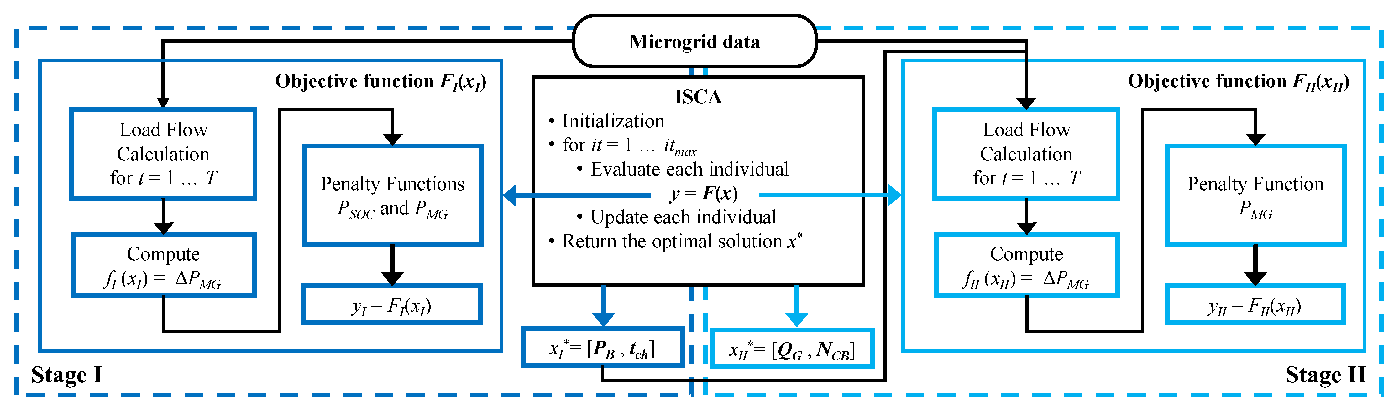
• Adaptation of the OARPC problem for metaheuristic solvers, consisting in performing the load flow calculation using a backward-forward sweep method and implementing penalty functions in order to assure that all the equality and inequality constraints are enforced. Furthermore, as the OARPC problem is solved in two successive stages, its increased complexity could significantly reduce the metaheuristic solver performance. The first stage focuses on optimizing the active power by scheduling the BESSs and EVs, then the second stage determines the optimal reactive power output of the DGs and CBs.
• Development of the Improved Sine-Cosine Algorithm, by introducing several mutation operators for enhancing both the exploration and exploitation phases’ performances.
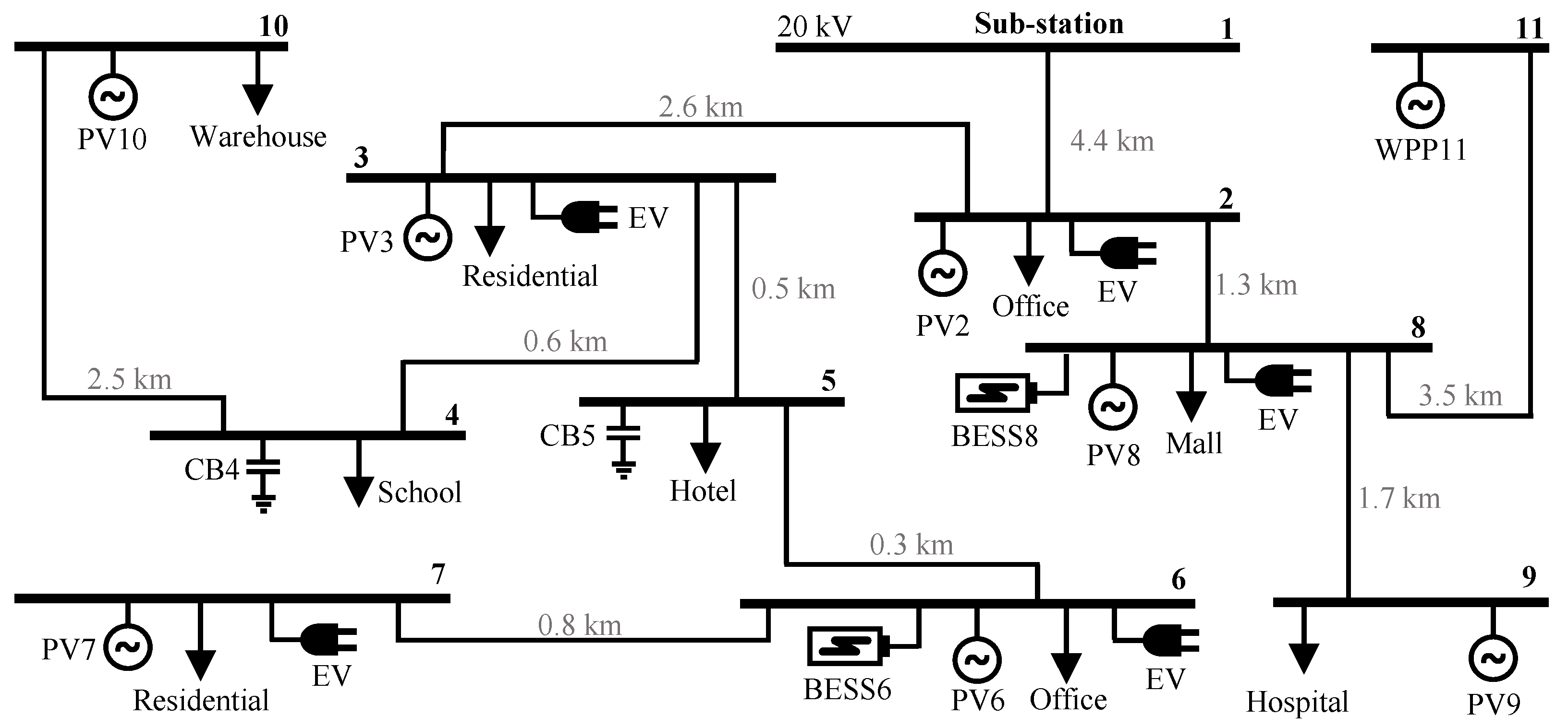
• It should also be mentioned, that the microgrid under study is proposed by the authors, inspired by the CIGRE MV Benchmark Network, and that all simulations presented in this study are conducted by using a software package developed by the authors under the Matlab environment.

The remainder of the paper is organized as follows. Section 2 presents the optimization problem formulation, while Section 3 describes the details of the mathematical model implementation. Section 4 contains the case studies and discussions of the results. Finally, Section 5 concludes the study.

2. Mathematical Model

This section describes the problem formulation for optimal operation scheduling within a microgrid. The microgrid is considered to consist of multiple types of loads, distributed generation (DGs), battery energy storage systems, electric vehicles, and capacitor banks (CBs). The detailed operational constraints of each microgrid component are presented as well.

2.1. Optimization Problem Formulation

Microgrids are defined by a high degree of renewable energy sources penetration, while integrating various loads and energy storage devices. The objective function considered in this paper is the minimization of the total active energy losses ΔW_MG within the microgrid for the considered scheduling time period T.

$$\begin{array}{l}\min f_{obj}\left(x\right)=\mathsf{\Delta }{W}_{MG}={\displaystyle \sum _{t=1}^T\mathsf{\Delta }{P}_{MG}^t}\cdot \mathsf{\Delta }t={\displaystyle \sum _{t=1}^T\left(P_{sl}^t+{\displaystyle \sum _{k=1}^{n_{GEN}}{P}_{G,k}^t}-{\displaystyle \sum _{k=1}^{n_N}{P}_{L,k}^t-{\displaystyle \sum _{k=1}^{n_{BESS}}{P}_{B,k}^t}}-{\displaystyle \sum _{k=1}^{n_{EV}}{P}_{EV,k}^t}\right)}\cdot \mathsf{\Delta }t\\ \mathrm{subject} \mathrm{to}: \begin{array}{c}g\left(x\right)=0\\ h\left(x\right)\le 0\end{array}\end{array}$$

(1)

where n_N is the number of microgrid buses, n_BESS is the number of BESS within the microgrid, and n_EV is the number of EVs. g(x) and h(x) are the equality and inequality restrictions that define the optimization model constraints.

During each time interval t, the active power losses $\mathsf{\Delta }{P}_{MG}^t$ are determined based on the active power exchanged by the microgrid with the upstream network $P_{sl}^t$, the active power supplied by the distributed generators and demanded by the load at each microgrid bus ($P_{G,k}^t$ and $P_{L,k}^t$), the active power exchanged by each BESS with the microgrid $P_{B,k}^t$ and the active power supplied to EV, $P_{EV,k}^t$.

The control variables vector consists of the active power exchanged between each BESS and the microgrid, the active power demanded by each EV, the reactive power provided by each distributed generator, and the operating step for each capacitor bank.

$$\left[x\right]=\left[\left[P_{B,1}\right]\dots \left[P_{B,k}\right]\dots \left[P_{B,n_{BESS}}\right],\left[t_{ch}\right],\left[Q_{G,1}\right]\dots \left[Q_{G,k}\right]\dots \left[Q_{G,n_{Gen}}\right],\left[N_{CB,1}\right]\dots \left[N_{CB,k}\right]\dots \left[N_{CB,n_{CB}}\right]\right]$$

(2)

$$\left[P_{B,k}\right]=\left[P_{B,k}^1 ,P_{B,k}^2 \dots P_{B,k}^t \dots P_{B,k}^T\right]$$

(3)

$$\left[t_{ch}\right]=\left[t_{ch,1} ,t_{ch,2} \dots t_{ch,k} \dots t_{ch,n_{EV}}\right]$$

(4)

$$\left[Q_{G,k}\right]=\left[Q_{G,k}^1 ,Q_{G,k}^2 \dots Q_{G,k}^t \dots Q_{G,k}^T\right]$$

(5)

$$\left[N_{CB,k}\right]=\left[N_{CB,k}^1 ,N_{CB,k}^2 \dots N_{CB,k}^t \dots N_{CB,k}^T\right]$$

(6)

where P_b,k is the power of kth BESS during time interval t, n_BESS is the number of BESS installed in the MG, and t_ch,k represents the required charging period for the kth EV. The reactive power generated by the kth DG in tth time interval is denoted by $Q_{G,k}^t$. Finally, $N_{CB,k}^t$ is the step of the kth capacitor bank during time period t.

2.2. Microgrid Modelling

In this paper, the constant active and reactive power model is used for all loads, distributed generators, batteries, and EVs while the constant shunt impedances model is applied for the capacitor banks.

The BESS is modelled using the exchanged active power and the State of Charge (SOC) of the battery, which is computed for each time interval t using the following equation:

$$SO{C}_k^t=SO{C}_k^{t-1}+\mathsf{\Delta }SO{C}_k^t$$

(7)

As it can be observed, SOC at tth period is calculated using the previous SOC and its variation between the two intervals, computed as:

$$\mathsf{\Delta }SO{C}_k^t=\frac{\mathsf{\Delta }{W}_k^t}{W_{max,k}^{}}=\{\begin{array}{l}\frac{P_{B,k}^t\cdot {\eta }_{Bch,k}\cdot \mathsf{\Delta }t}{W_{max,k}^{}} \mathrm{if} P_{B,k}^t\ge 0\\ \frac{P_{B,k}^t\cdot \mathsf{\Delta }t}{W_{max,k}^{}\cdot {\eta }_{Bdsc,k}} \mathrm{if} P_{B,k}^t<0\end{array}$$

(8)

where ${\eta }_{Bch,k}$ and ${\eta }_{Bdch,k}$ are the charging and discharging efficiencies of kth BESS, while W_max,k denotes its capacity.

The optimal charging schedule for the considered number of n_EV electrical vehicles is determined within the optimization problem by providing, for each EV, the charging starting time t_start,k. In this regard, the electrical vehicles are modelled individually, considering that each EV arrives at the charging station at the arrival time t_arr,k with an initial energy level of W_init,k and requires to be charged to the desired energy level W_fin,k until its departure time t_dep,k. The active power P_ch,k demanded by each EV is considered constant during the charging period Δt_ch. Therefore, the charging period Δt_ch and charging stopping time t_stop will be determined as follows:

$$\mathsf{\Delta }{t}_{ch,k}=\frac{W_{fin,k}-W_{init,k}}{P_{ch,k}\cdot {\eta }_{EVch,k}}$$

(9)

$$t_{stop,k}=t_{start,k}+\mathsf{\Delta }{t}_{ch,k}$$

(10)

Consequently, the EV active power demand is equal to P_ch,k value during the charging period and zero for the rest of the scheduling window:

$$P_{EV,k}^t=\{\begin{array}{l}{P}_{ch,k} \mathrm{if} t_{start,k}\le t\le t_{stop,k}\\ 0 \mathrm{otherwise} \end{array}$$

(11)

2.3. Equality Constraints

The microgrid optimal scheduling must be performed based on power flow simulations. The equality constraints presented in Equation (12) consist of the active and reactive power balance equations at each bus, used in the power flow computation.

$$\begin{array}{cc}\begin{array}{l}{P}_{G,i}^t-P_{L,i}^t-V_i^t{\displaystyle \sum _{k=1}^{n_N}{V}_k^t\left[G_{ik}\cos \left({\theta }_i^t-{\theta }_k^t\right)+B_{ik}\sin \left({\theta }_i^t-{\theta }_k^t\right)\right]=0}\\ Q_{G,i}^t-Q_{L,i}^t-V_i^t{\displaystyle \sum _{k=1}^{n_N}{V}_k^t\left[G_{ik}\sin \left({\theta }_i^t-{\theta }_k^t\right)-B_{ik}\cos \left({\theta }_i^t-{\theta }_k^t\right)\right]=0}\end{array}& ,\forall i=1\dots n_N\end{array}$$

(12)

2.4. Inequality Constrains

The inequality constraints in the optimal scheduling problem involve the microgrid’s component limits and their operational restrictions. As previously mentioned, the model presented in this paper considers battery energy storage systems, electric vehicles, generators, and capacitor banks. Moreover, the bus voltages and line rating are considered as well.

2.4.1. Battery Energy Storage System Constraints

Considering n_ESS the number of BESS installed in the microgrid, the exchanged power of each BESS with the microgrid must be contained within the maximum charging and discharging capacity at each time interval t.

$$P_{B,k}^{min}\le P_{B,k}^t\le P_{B,k}^{max},\forall k=1\dots n_{ESS}$$

(13)

The state of charge (SOC) for each battery at any given time interval t is restricted to exceed its minimum and maximum limits, in order to extend BESS lifetime.

$$SO{C}_k^{min}\le SO{C}_k^t\le SO{C}_k^{\max }$$

(14)

The microgrid optimization is performed in a 24-h analysis framework in this paper. To preserve the SOC for the following days, the difference between the SOC at the end of the scheduling window and the SOC at the beginning of the process should not exceed a tolerance value.

$$\left|SO{C}_k^0-SO{C}_k^T\right|\le {\epsilon }_{SOC}$$

(15)

In this paper, the considered acceptable difference between initial and final SOC for each BESS is 5%.

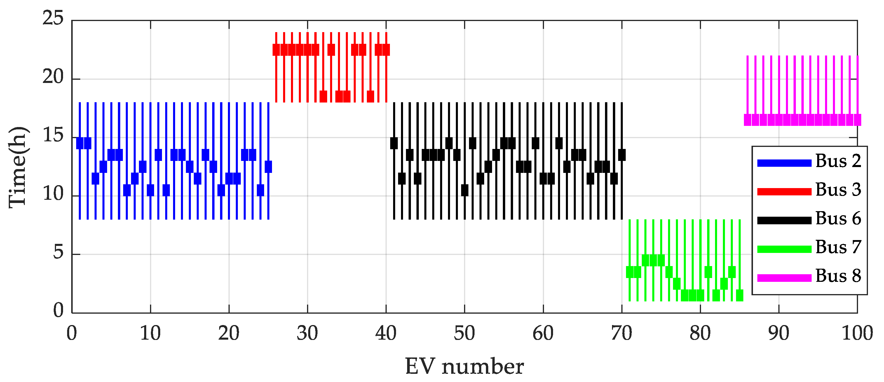
2.4.2. Electric Vehicles Constraints

As previously mentioned, EVs are modelled as a fixed absorbed power during the charging time $\mathsf{\Delta }{t}_{ch,k}$. The charging of the EV must commence after its arrival time $t_{arr,k}$ at the charging station. Moreover, at the established departure time, the EV must reach its full battery capacity, therefore the time span between the charging starting point and departure time must cover the necessary charging duration $\mathsf{\Delta }{t}_{ch,k}$.

$$t_{arr,k}\le t_{start,k}\le t_{dep,k}-\mathsf{\Delta }{t}_{ch,k},\forall \mathrm{k}=1\dots {\mathrm{n}}_{EV}$$

(16)

2.4.3. Generator Constraints

Disregarding the generation source (PV, wind), each distributed generator’s reactive power has an imposed minimum and maximum value.

$$Q_{G,k}^{min}\le Q_{G,k}^t\le Q_{G,k}^{max} ,\forall k=1\dots n_{Gen}$$

(17)

The reactive power limits are computed using the generated active power and the operational power factor.

2.4.4. Capacitor Banks Constraints

The operating step of the capacitor banks must be within the minimum and maximum values.

$$N_{CB,k}^{min}\le N_{CB,k}^t\le N_{CB,k}^{max} , \forall k=1\dots n_{CB}$$

(18)

2.4.5. Microgrid Operational Constraints

The bus voltages must be between the lower and upper bound, to ensure the security of the power supply.

$$V_k^{min}\le V_k^t\le V_k^{max} ,\forall k=1\dots n_N$$

(19)

Electrical line current must not exceed the thermal limit in the microgrid operation thus, the following constraint is imposed:

$$\left|I_k^t\right|\le I_k^{max} ,\forall k=1\dots n_L$$

(20)

2.5. Improved Sine Cosine Algorithm

The Sine Cosine Algorithm (SCA) represents a metaheuristic algorithm proposed by S. Mirjalili [27] for solving global optimization problems. The algorithm relies on the trigonometric functions sine and cosine to find the optimal solution in the search space through an iterative process. Due to its numerous advantages, the SCA earned the attention of the research community. In [28], the authors addressed the reactive power dispatch problem in transmission systems employing the SCA, achieving better performances compared to other metaheuristic algorithms, such as Particle Swarm Optimization and Whale Optimization Algorithm. SCA is employed in [29] to optimize the peak operation problem of hydropower reservoirs. Authors of [30] solved the optimal power flow for the IEEE-30 bus test system using SCA, while in [31] the optimal sizing and placement of BESS in a distribution network is determined using the Sine Cosine Algorithm and the Arithmetic Optimization Algorithm.

Belonging to the population-based class of metaheuristic algorithms, the Sine Cosine Algorithm first produces N initial random solutions. Considering a problem consisting in m variables, $X_i^j$ the position in the ith dimension of the jth solution, where X^j = [$X_1^j$, $X_2^j$ …,$X_m^j$], the solutions are updated throughout the iterative search process using the following equation:

$$X_i^{j,t+1}=\{\begin{array}{cc}\begin{array}{l}{X}_i^{j,t}+r\times \sin (ran{d}_1)\times \left|ran{d}_2\times P_i^t-X_i^{j,t}\right|,\\ X_i^{j,t}+r\times \cos (ran{d}_1)\times \left|ran{d}_2\times P_i^t-X_i^{j,t}\right|,\end{array}& \begin{array}{l}ran{d}_3<0.5\\ ran{d}_3\ge 0.5\end{array}\end{array}$$

(21)

where $P_i^t$ is the known best position in dimension i at the current iteration t within the search space, defined as the destination. The parameter rand₁ is randomly generated in the [0, 2π] range, determining the direction of the solution movement in relation to the destination position. Parameter rand₂, generated in [0, 2] range, adds a random weight to the destination position to increase or decrease its influence in the current solution’s position, while parameter rand₃ is produced using a uniformly distributed distribution in the interval [0, 1], imposing the use of either sine or cosine function [32]. Parameter r is determined using the following equation:

$$r=\lambda -t\frac{\lambda }{T_{\max }}$$

(22)

where t is the current iteration, T_max is the total number of iterations considered, while λ is a constant value. In this paper, the value of λ was set to 2.

Among its advantages, SCA involves a low number of parameters, therefore the fine-tuning process is not critical. Due to its simplicity, the algorithm presents high robustness and good simulation time [33]. In order to achieve better performance of the SCA, a mutation operator is implemented in this paper to improve the exploration phase of the algorithm. The proposed operator consists of modifying a number of N_mut existing solutions. For the selected solutions, the mutation operator applies one of the mechanisms, according to the ISCA pseudocode presented in Algorithm 1.

Algorithm 1. Improved Sine-Cosine Algorithm

1. Initialize population of N solutions  2. For t = 1: Tmax  3.  Update the N solutions’ position according to Equation (21) in iteration t.  4.  Determine the percentage of mutated solutions (in 5…35% range):  $N_{mut}=N\times \frac{\mathrm{mod}(t,50)+5}{100}$  5.  For i = 1: Nmut  6.      Choose two random positions pos1 and pos2 of the ith solution.

7.      Generate a random number p in [0, 1] range.  8.      If p ≤ 0.2  $\begin{array}{l}{X}_{po{s}_1}^{i,t}=rand\times (u{b}_{po{s}_1}-l{b}_{po{s}_1})+l{b}_{po{s}_1}\\ X_{po{s}_2}^{i,t}=rand\times (u{b}_{po{s}_2}-l{b}_{po{s}_2})+l{b}_{po{s}_2}\end{array}$  9.      Else if p ≤ 0.8

$\begin{array}{l}{X}_{po{s}_1}^{i,t}=P_{po{s}_1}^t+(rand\times (u{b}_{po{s}_1}-l{b}_{po{s}_1})+l{b}_{po{s}_1})\\ X_{po{s}_2}^{i,t}=P_{po{s}_2}^t-(rand\times (u{b}_{po{s}_2}-l{b}_{po{s}_2})+l{b}_{po{s}_2})\end{array}$

10.     Else

$\begin{array}{l}{X}_{po{s}_1}^{i,t}=P_{po{s}_1}^t+rand\times (u{b}_{po{s}_1}-l{b}_{po{s}_1})+l{b}_{po{s}_1}\\ X_k^i=P_k^t-(rand\times (u{b}_k-l{b}_k)+l{b}_k)/(m-1) \forall \mathrm{k}=1\dots \mathrm{m}, \mathrm{k}\ne {\mathrm{pos}}_1\end{array}$

11.   end  12. end

As it can be observed, the percentage of mutated solutions linearly decreases as the iterations proceed. However, at a certain number of iterations (50 proposed in this paper), parameter N_mut resets its initial value, repeating the process. In this manner, the algorithm’s ability to avoid local optima is improved.

3. Model Implementation

In this section, the two-stage coordination model for the microgrid and the metaheuristic solver approach are outlined, including the implementation of penalty functions for the objective functions. Finally, the simulation framework is presented, describing the proposed algorithm.

3.1. Two Stage Active-Reactive Power Coordinated Optimization

The optimization problem formulated in this study, aiming at the minimization of microgrid’s active energy losses for a one-day scheduling window, is solved using a metaheuristic algorithm, namely the improved SCA, that determines the optimal EV charging period, BESS scheduling, and the optimal reactive power support provided by the distributed generators and capacitor banks.

Considering that the one-day analysed period is divided into T time intervals, for each interval t, the algorithm needs to determine:

• the active power exchange between each of the n_BESS battery energy storage systems $P_{B,k}^t$ (n_BESS × T variables);
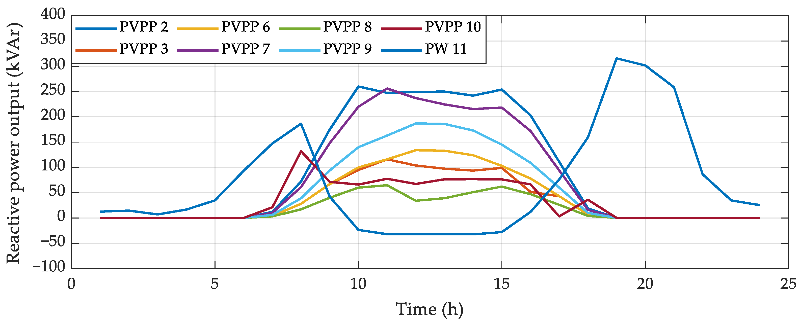
• the reactive power output for each distributed generators $Q_{G,k}^t$ (n_GEN × T variables);
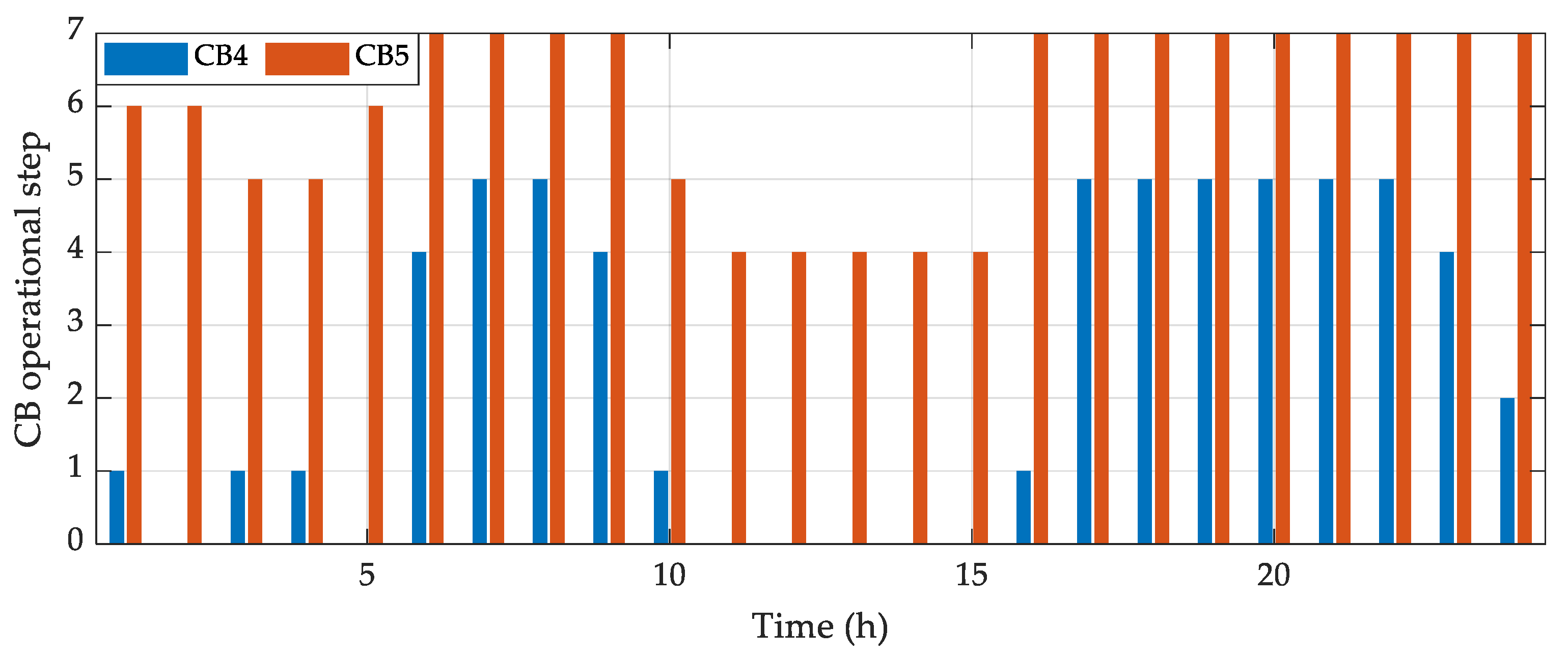
• operational step for each of the n_CB capacitor banks $N_{CB,k}^t$ (n_CB × T variables);
• the charging starting time for each electrical vehicle (n_EV variables).

As a significant number of research papers demonstrate, metaheuristic solvers usually provide high performances in solving multi-dimensional real-world optimization problems [34]. However, for the particular case of the OARPC problem, the relatively large number of control variables substantially increases the problem’s complexity, resulting in a considerable decrease in convergence speed. Generally, solving high-complexity problems requires a large population size and a number of iterations, in order to ensure the necessary computational effort. Given that in the proposed optimization model the reactive power support is dependent upon the active power scheduling, the risk of the metaheuristic solver converging to a local optimum is severely increased. Therefore, simply expanding the population size and iterations does not completely mitigate this risk. In this regard, this paper proposes a two-stage approach to solving the OARPC problem.

The first stage minimizes the active energy losses during the one-day period by determining the optimal scheduling for BESSs and EVs.

$$\begin{array}{l}\min f_I\left(x_I\right)=\mathsf{\Delta }{W}_{MG}={\displaystyle \sum _{t=1}^T\mathsf{\Delta }{P}_{MG}^t}\cdot \mathsf{\Delta }t={\displaystyle \sum _{t=1}^T\left(P_{sl}^t+{\displaystyle \sum _{k=1}^{n_{GEN}}{P}_{G,k}^t}-{\displaystyle \sum _{k=1}^{n_N}{P}_{L,k}^t-{\displaystyle \sum _{k=1}^{n_{BESS}}{P}_{B,k}^t}}-{\displaystyle \sum _{k=1}^{n_{EV}}{P}_{EV,k}^t}\right)}\cdot \mathsf{\Delta }t\\ \mathrm{subject} \mathrm{to}: \begin{array}{c}{g}_I\left(x_I\right)=0\\ h_I\left(x_I\right)\le 0\end{array}\end{array}$$

(23)

For the first stage, the control variables vector x_I contains the BESS active power exchange and the EV charging start time:

$$\left[x_I\right]=\left[P_{B,1}^1\dots P_{B,1}^t \dots P_{B,1}^T , P_{B,k}^1\dots P_{B,k}^t \dots P_{B,l}^T, P_{B,n_{BESS}}^1\dots P_{B,n_{BESS}}^t \dots P_{B,n_{BESS}}^T, t_{ch,1}\dots t_{ch,k} \dots t_{ch,n_{EV}}\right]$$

(24)

The equality constraints for the first stage g_I(x_I) from Equation (23) consist of the nodal active and reactive power equations, described by Equation (12). The first stage inequality constraints h_I(x_I) consist of the BESS active power and SOC limitations from Equations (13)–(15), the charging start time constraint shown in Equation (16), and the microgrid operational constraints defined by Equations (19) and (20).

The second stage minimizes the active energy losses by determining the optimal reactive power output for the DGs and CBs.

$$\begin{array}{l}\min f_{II}\left(x_{II}\right)=\mathsf{\Delta }{W}_{MG}={\displaystyle \sum _{t=1}^T\mathsf{\Delta }{P}_{MG}^t}\cdot \mathsf{\Delta }t={\displaystyle \sum _{t=1}^T\left(P_{sl}^t+{\displaystyle \sum _{k=1}^{n_{GEN}}{P}_{G,k}^t}-{\displaystyle \sum _{k=1}^{n_N}{P}_{L,k}^t-{\displaystyle \sum _{k=1}^{n_{BESS}}{P}_{B,k}^t}}-{\displaystyle \sum _{k=1}^{n_{EV}}{P}_{EV,k}^t}\right)\cdot \mathsf{\Delta }t}\\ \mathrm{subject} \mathrm{to}: \begin{array}{c}{g}_{II}\left(x_{II}\right)=0\\ h_{II}\left(x_{II}\right)\le 0\end{array}\end{array}$$

(25)

The control variables vector for the second stage of the OARPC problem, x_II, consists of the reactive power output for each DG and operational step for each CB during each time interval t.

$$\left[x_{II}\right]=\left[\left[x_{II}^1\right],\left[x_{II}^2\right]\dots \left[x_{II}^t\right]\dots \left[x_{II}^T\right]\right]$$

(26)

$$\left[x_{II}^t\right]=\left[Q_{G,1}^t ,Q_{G,2}^t \dots Q_{G,k}^t \dots Q_{G,n_{Gen}}^t, N_{CB,1}^t ,N_{CB,2}^t \dots N_{CB,k}^t \dots N_{CB,n_{CB}}^t\right]$$

(27)

The second stage equality constraints g_II(x_II) given in Equation (25) also consist of the nodal active and reactive power equations from Equation (12). The inequality constraints for the second stage h_II(x_II) consist of the operational limitations of DGs reactive power output, CBs operational step, and microgrid bus voltage and current limits, presented in Equations (17)–(20).

3.2. Adaptations for Metaheuristic Solvers

The OARPC problem formulated in this paper is solved using the proposed Improved Sine-Cosine Algorithm, therefore several adaptations are required in order to assure that the equality and inequality constraints are satisfied.

3.2.1. Equality Constraints Integration

The equality constraints for both stages g_I(x_I) and g_II(x_II) are satisfied by performing the load flow calculation during the objective function evaluation. Generally, this technique is applied for metaheuristic solvers in order to avoid introducing a large number of variables (i.e., bus voltages magnitude V and angle θ) from the active and reactive power equations given in Equation (12). In this paper, the backward-forward sweep method (BFS) is applied for the load flow calculation, as this method provides superior performances in comparison to the Newton−Raphson and Seidel−Gauss methods on radial and tree-like distribution networks (including microgrids) with high R/X ratios [35].

The BFS consists of two main steps, starting with the backward sweep followed by the forward sweep, repeated through an iterative process. However, the network topology requires a pre-processing stage based on graph theory, in order to determine the predecessor and successor for each network node and the visiting order of all network buses. The BFS begins with the initialization that consists in considering all bus voltages V_k equal to the slack bus voltage V_sl, and all bus voltages angles equal to zero. During the first step, namely the backward sweep, the currents demanded at each bus and the current flows through the branches are determined starting with the terminal nodes and advancing towards the slack bus. Afterwards, in the forward sweep, the voltage drops on branches, and bus voltages are determined starting from the slack bus [36]. Finally, the iterative process is repeated until the convergence test, consisting in comparing the slack bus power of the latest two iterations, is satisfied.

3.2.2. Inequality Constraints Integration

As the first stage of the OARPC optimizes the active power scheduling and the second stage optimizes the reactive power control devices, the inequality constraints are integrated differently into the two stages. During the first stage, the inequality constraints g_I(x_I) from Equation (23) regarding BESS active power exchange and the EV charging starting time are integrated as upper and lower bounds of the corresponding control variables. The inequality constraints regarding the SOC values, depicted in Equations (14) and (15), are enforced by introducing a penalty function P_SOC, defined as follows:

$$P_{SOC}={\displaystyle \sum _{k=1}^{n_{BESS}}\left({\displaystyle \sum _{t=1}^T\left(p_{SOC1,k}^t\right)}\right)}+{\displaystyle \sum _{k=1}^{n_{BESS}}\left(p_{SOC2,k}\right)}$$

(28)

Parameter $p_{SOC1,k}^t$ represents the penalty coefficient for the kth BESS during the tth time interval, applied to enforce the $SO{C}_k^{min}$ and $SO{C}_k^{\max }$ by increasing its value proportionally to the limit violation:

$$p_{SOC1,k}^t=\{\begin{array}{c}SO{C}_k^{min}-SO{C}_k^t, \mathrm{if} SO{C}_t<SO{C}_k^{min}\hfill \\ 0,\mathrm{if} SO{C}_k^{min}\le SO{C}_k^t\le SO{C}_k^{\max }\hfill \\ SO{C}_k^t-SO{C}_k^{\max }, \mathrm{if} SO{C}_k^t>SO{C}_k^{\max }\hfill \end{array}$$

(29)

The second penalty coefficient $p_{SOC2,k}$ is used to enforce the BESS charging-discharging balance constraint for the kth BESS:

$$P_{SOC2,k}=\{\begin{array}{c}\begin{array}{l}\left|SO{C}_k^0-SO{C}_k^T\right|, \mathrm{if} \left|SO{C}_k^0-SO{C}_k^T\right|>{\epsilon }_{SOC}\\ 0,\mathrm{if} \left|SO{C}_k^0-SO{C}_k^T\right|\le {\epsilon }_{SOC}\end{array}\end{array}$$

(30)

The inequality constraints in Equations (19) and (20) regarding the microgrid operational bus voltage and branch currents limits are enforced by the P_MG penalty function:

$$P_{MG}={\displaystyle \sum _{t=1}^T{\displaystyle \sum _{k=1}^{n_N}{p}_{V,k}^t+}}{\displaystyle \sum _{t=1}^T{\displaystyle \sum _{k=1}^{n_L}{p}_{I,k}^t}}$$

(31)

The penalty coefficients $p_{V,k}^t$ and $p_{I,k}^t$ have increased values if, during the tth interval, the bus voltage limits at the kth bus are violated or the kth line current exceed the capacity:

$$\begin{array}{ccc}{p}_{V,k}^t=\{\begin{array}{c}{V}_k^{min}-V_k^t, \mathrm{if} V_k^t<V_k^{min}\\ 0,\mathrm{if} V_k^{min}\le V_k^t\le V_k^{max}\\ V_k^t-V_k^{max}, \mathrm{if} V_k^t>V_k^{max}\end{array}& \mathrm{and}& p_{I,k}^t=\{\begin{array}{c}\begin{array}{l}{I}_{I,k}^t-I_k^{max}, \mathrm{if} I_{I,k}^t>I_k^{max}\\ 0,\mathrm{if} I_{I,k}^t\le I_k^{max}\end{array}\end{array}\end{array}$$

(32)

The second stage of the OARPC problem focuses on the reactive power control devices, namely the DGs and the CBs within the microgrid. The DGs reactive control limits and CBs operational step limits, given in Equations (17) and (18), are integrated as lower and upper bounds for the control variables $Q_{G,k}^t$ and $N_{CB,k}^t$, while the microgrid operational constraints are enforced using the P_MG penalty function defined in Equations (31) and (32).

During the optimization process, occurrences of divergent load flow solutions are possible, therefore a large penalty coefficient w_LF is introduced to assure that only viable load flow solutions are considered. On the other hand, weights w are introduced for the penalty functions in order to assure that the penalized individuals have a considerable numerical handicap in comparison to the viable individuals. Finally, the penalized objective functions for the two stages F_I and F_II are defined as follows:

$$F_I(x_I)=w_{LF}\cdot \left(f_I\left(x_I\right)+w_{SOC}\cdot P_{SOC}+w_{MG}\cdot P_{MG}\right)$$

(33)

$$F_{II}(x_{II})=w_{LF}\cdot \left(f_{II}\left(x_{II}\right)+w_{MG}\cdot P_{MG}\right)$$

(34)

3.3. Simulation Framework

The simulations presented in this paper are performed using a software toolbox developed by the authors under the Matlab environment. The toolbox is structured into three modules. The data input module gathers the microgrid data, the load and generation curves for the different load types, and distributed generators within the microgrid. The optimization module comprises the objective and penalty functions, the load flow calculation function, developed by the authors based on the backward-forward sweep method, alongside the two considered metaheuristic solvers, namely the ISCA, which is developed by the authors and the original SCA code developed by S. Mirjalili in [27]. This module provides the user with the possibility of performing the OARPC for a one-day period, or for the entire year by using the ISCA or the SCA and saves the results in a “.mat” file. The post-processing module loads the results provided by the optimization module and generates various analyses, and statistics in both numerical and graphical form.

The active−reactive power coordinated optimization problem is solved by the optimization module in two consecutive stages, as the flowchart in Figure 1 shows. Firstly, the active power optimization is performed by applying ISCA or SCA for minimizing the penalized objective function F_I(x_I) by determining the optimal scheduling for the BESSs and EVs charging time. The results provided by the first stage x_I^*, consist of the BESS active power during the day P_B and EV charging time t_ch. Afterwards, the objective function F_II(x_II) is minimized under the second stage by determining the optimal reactive power output of the DGs and CBs within the microgrid. The second stage input data consists of the microgrid operational data, including the results provided by the first stage. Finally, the second stage results x_II^* consisting of the DGs reactive power output Q_G and CBs operational steps are returned alongside the first stage results x_I^* as the solution to the OARPC problem.

It should be mentioned that the second stage control variables on different time intervals are independent, therefore, the reactive power optimization is performed individually for each time interval t in order to reduce the problem’ s complexity for the metaheuristic solvers.

4. Case Study

4.1. Network under Study

The microgrid considered for this study is inspired by the 20 kV CIGRE MV benchmark network presented in [26], consisting of 11 buses among which bus 1 represents the connection point to the upstream network. The considered microgrid comprises ten underground electrical cables that form a tree-like topology, as the one-line diagram presented in Figure 2 shows. The microgrid operates in the grid-connected mode, as it supplies nine loads while also integrating two battery energy storage devices, seven photovoltaic power plants (PVPPs), one wind power plant (WPP), two CBs, and five EV charging stations.

The microgrid electrical lines are equipped with an identical medium voltage underground electrical cable, that presents the following parameters: resistance r₀ = 0.927 Ω/km, reactance x₀ = 0.142 Ω/km, susceptance b₀ = 47.124 μS/km and rated current I_max = 150 A, extracted from [26].

The line lengths are shown in Figure 2, while the data referring to all the other devices are presented in

Table 1. Microgrid data.

Bus Number	Load Type	PL,max (kW)	QL,max (kVAr)	nEV (–)	tarr–tdep (hhmm)	DG Type	PG,max (kW)	QG,max (kVAr)	WB,max (kWh)	PB,max (kW)	NCB × QCB,r (kVAr)
1	–	–	–	–	–	–	–	–	–	–	–
2	Office	825	615	25	700–1659	PVPP	650	315	–	–	–
3	Residential	625	385	15	1700–2359	PVPP	250	121	–	–	–
4	School	145	105	–	–	–	–	–	–	–	5 × 50
5	Hotel	370	250	–	–	–	–	–	–	–	7 × 50
6	Office	880	555	30	700–1659	PVPP	250	121	900	225	–
7	Residential	925	650	15	000–759	PVPP	550	266	–	–	–
8	Mall	250	180	15	1500–2159	PVPP	150	73	600	150	–
9	Hospital	305	225	–	–	PVPP	350	170	–	–	–
10	Warehouse	175	135	–	–	PVPP	1200	581	–	–	–
11	–	–	–	–	–	WPP	1600	775	–	–	–

.

In the table above, P_L,max and Q_L,max are the maximum active and reactive demanded powers, n_EV is the number of EVs with their arrival t_arr and departure t_dep times, alongside the DG type, maximum active P_G,max, and reactive Q_G,max power. The BESS maximum active power and total energy capacity are denoted by P_B,max and W_B,max, respectively, while for the CB, the number of steps and their rated reactive power per step are represented by N_CB and Q_CB,r.

The load profiles for all the load types supplied by the considered microgrid are obtained from the OpenEI database [37], while the generation curves for the PVPPs and WPP are extracted from the Renewables Ninja database [38,39,40]. The geographical area of Atlanta, Georgia, USA was considered for both load and generation curves, which were obtained for a one-year period with one-hour granulation.

Each EV is considered to require a charging duration of 2 h at a constant active power of 30 kW each, for simplification purposes. Also, the arrival and departure times are considered equal for all the EVs connected to a charging station.

4.2. ISCA Performance Analysis

This section presents a performance comparison between the ISCA and the original SCA in solving each stage of the OARPC problem separately.

Firstly, a performance analysis is presented for the first stage of the OARPC problem, which consists of the active power scheduling by optimally scheduling the two BESSs and the 100 considered EVs charging. For this purpose, a comparison is conducted between the results provided by both ISCA and SCA in 10 consecutive runs, with a set of identical parameters. The average objective value f_obj and average running time t_run obtained by each algorithm for each set of parameters are centralized in

Table 2. Performance comparison between ISCA and SCA.

N	Tmax	trun (s)		Δtrun (%)	fobj		Δfobj (%)
		ISCA	SCA		ISCA	SCA
50	50	8.4	8.3	1.0%	111.0	362,647.8	N/A
100	100	34.1	33.1	2.8%	98.3	107.7	−9.5%
150	150	74.5	73.1	2.0%	87.0	105.9	−21.7%
200	200	134.7	131.2	2.6%	84.4	101.7	−20.6%
250	250	212.1	206.4	2.7%	82.0	100.9	−23.1%
300	300	308.7	295.9	4.2%	79.9	100.0	−25.1%
350	350	414.7	395.2	4.7%	79.4	97.2	−22.4%

, alongside the percentage variation, denoted Δf_obj and Δt_run, between the f_obj and t_run values obtained by each algorithm. It should be mentioned that the simulations were performed using a PC equipped with an AMD Ryzen 7 2700 Eight-Core Processor at 3.20 GHz and 32GB of RAM.

The results show that, for each set of parameters, ISCA obtains an increase in performance between 9.5%, for N = 100 and T_max = 100, and 25.1% for N = 300 and T_max = 300, relative to the SCA. On the other hand, the increased complexity of the ISCA model leads to 1.0–4.7% longer running times, relative to the SCA. However, the proposed improvements provide the ISCA with superior performances in both the exploration and exploitation phases, resulting in a significant increase in performance at the expense of a relatively longer running time.

The relatively large number of variables for the first stage 100 + 2 × 24 = 148, resulting from scheduling 100 EVs and two BESS for 24 time intervals during each day, requires increased computational effort in order to deliver good quality results. As it can be observed, for N = 50 and T_max = 50 the SCA obtains only obtains a feasible solution in 6 out of 10 simulations, resulting in an enormous average f_obj value, therefore the Δf_obj has not been computed. By comparison, the ISCA obtains 100% feasible solutions for identical N and T_max values. Furthermore, the ISCA performance improvement resulted from the increase in population size and iterations decrease from 11.4% between the first two sets of N and T_max values to 0.6% between the final two N and T_max sets. Finally, the population size of N = 350 individuals and iterations number T_max = 350 are chosen for the first stage, as a sufficient computation effort is provided to the ISCA for providing consistent performance.

In the second part of this section, the performance analysis is conducted by employing both algorithms for solving both stages of the OARPC problem during each day of the year, with identical parameters.

The second stage performs the reactive power planning by determining the optimal reactive power output of the seven PVPPs, one WPP, and two CBs, during each one-hour time of the considered day. As the control variables from different time intervals are independent, the second stage is solved separately for each time interval. In this manner, the number of control variables for the metaheuristic solvers is reduced to 7 + 1 + 2 = 10 when each hour of the day is optimized separately, in comparison to 24 × 10 = 240 when the entire day is optimized at once. For this reason, the population size and iteration number are reduced to N = 150 and T_max = 150.

The performance analysis is conducted by comparing the optimal objective function determined by each algorithm, consisting of the daily active energy losses. However, as the active power demanded by the load and supplied by the DGs has a significant variation during the year, the daily energy losses are also subject to variations. Therefore, the results are presented in Figure 3 as the objective function f_obj variation, obtained by the ISCA, expressed in percentage relative to the classic SCA.

The results shown in Figure 3 reveal that the ISCA is superior to the SCA in terms of performance, as the objective function values are reduced by at least 3.55% during each day of the year. For a number of 257 days the f_obj values are lower by at least 10%, while an improvement of at least 15% is observed for 141 days, and a reduction of at least 20% for 35 days. The largest difference between the ISCA and SCA reaches 31.1% for solely one day. On average, a reduction of the active energy losses during the year period of 12.6% is obtained by applying the Improved Sine-Cosine Algorithm, instead of the classical SCA. In conclusion, the performance analysis revealed that the ISCA is superior to the SCA in solving the OARPC problem.

4.3. Results and Discusion

This section presents the results determined by solving the OARPC problem using the Improved Sine-Cosine Algorithm, while a reference scenario based on a local control strategy is also developed as a term of comparison for evaluating the OARPC performance.

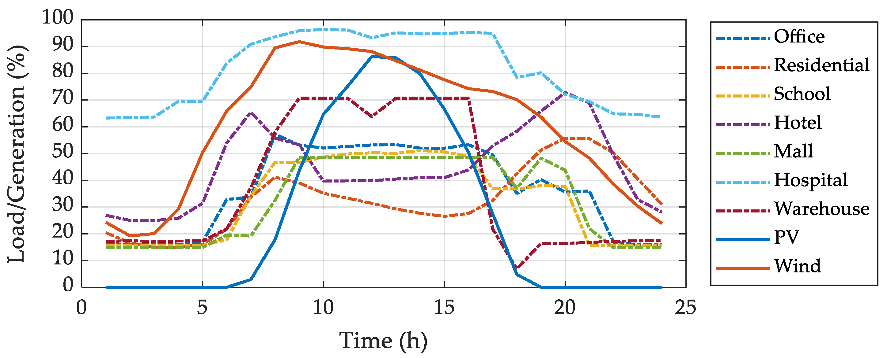
4.3.1. Microgrid Operational Conditions

This section presents a detailed analysis regarding the microgrid operation for a one-day period considering the proposed two-stage active reactive power dispatch. For this purpose, a spring day was selected for evaluation, as it is characterized by a medium load demand, a medium PVPP active power output, and a relatively high WPP generation.

The load curve for the seven considered load types is presented in Figure 4 alongside the generation curve for the PVPPs and WPP. It should be mentioned that an identical load curve is applied for both residential loads, connected at buses 3 and 7, and for both Office loads supplied from buses 2 and 6. In this manner, the PVPP generation curve shown in Figure 4 is applied to all seven PVPPs within the microgrid, given their geographical proximity.

It should be mentioned that time intervals considered in this study have a one-hour duration, and the numbering begins at 1, therefore, the 1st time interval is comprised between 0⁰⁰ and 0⁵⁹, and the 24th interval between 23⁰⁰ and 23⁵⁹.

The aggregated load curve for all the loads within the considered microgrid presents two peaks, namely the morning and evening peaks which occur in the 8th and 19th time intervals, with a total demanded active power of 2356 kW and 2175 kW, respectively. Given that a constant power factor is considered for all loads, the reactive power demand peaks of 1631 kVAr and 1497 kVAr coincide with the aforementioned active power demand peaks.

The generation curve shows that the PVPPs maximum active power output reaches 2932 kW in the 12th time interval, representing 86.2% of the total installed capacity, while the WPP generates between 307.6 kW at 3⁰⁰ and 1469 kw at 9⁰⁰, which represents between 19.2% and 91.8% of its capacity.

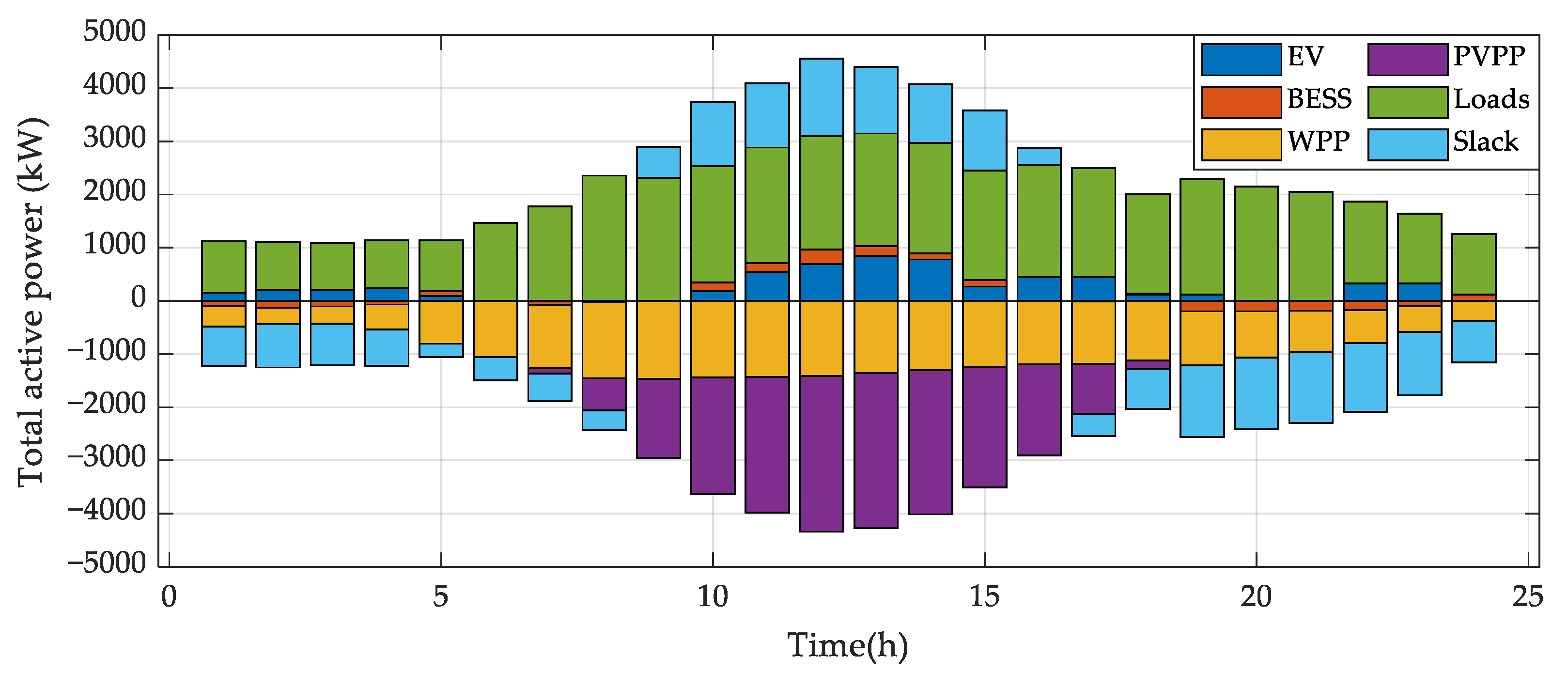
4.3.2. Centralized Active-Reactive Power Optimization for the Selected Day

The two-stage OAPRC is solved for the selected day by applying the Improved Sine-Cosine Algorithm with further increased population size and iterations number in order to provide the ISCA with sufficient computational power for fine tuning the results. As the optimal coordination model aims at the efficient management of all microgrid components, the proposed approach represents a centralized control strategy. The first stage, consisting of the active power coordinated optimization, provides the optimal scheduling for the two BESSs and 100 EVs charging in order to minimize the daily active energy losses. Considering the increased complexity of this stage, given by the relatively large number of 2 × 24 + 100 = 148 control variables, the population size of N = 1000 individuals and iterations number of T_max = 1000 were considered for the ISCA. The EV scheduling determined after the first stage of the OARPC is presented in Figure 5, where each thin vertical line represents the EV parking time, while the thicker line shows the actual charging time, while the EV connection bus is given by the line’s colour.

The active power demanded by the loads is minimum until 5⁰⁰, when it begins to constantly increase up to the maximum value of 2356 kW (in the 7⁰⁰–8⁰⁰ interval), therefore all 15 EVs connected at bus 7 are scheduled to fully charge until 5⁰⁰, while the other 3 are fully charged until 6⁰⁰. In a similar manner, 11 out of the 15 EVs connected at bus 3 are charging between 21⁰⁰–23⁰⁰ as the load demand is reducing from 2049 kW in the 20⁰⁰–21⁰⁰ interval to 1536 kW and 1307 kW in the following two hours.

All EVs connected to the charging station at bus 8 are available for charging between 15⁰⁰ and 22⁰⁰. The optimal active power planning schedules all 15 EVs at the bus to charge 8 between 15⁰⁰ and 17⁰⁰, as during this second period of the day both PVPP and WPP generation are decreasing, providing the microgrid with an active power surplus only until 17⁰⁰.

All 55 electrical vehicles charging at the two Office buildings connected by buses 2 and 6 are scheduled between 9⁰⁰ and 15⁰⁰. During the 9⁰⁰–15⁰⁰ interval the highest PVPP and WPP generation occurs, with a total active power output comprised between 3508 kW and 4341 kW, while the total load demand is relatively constant with values between 2190 kW and 2057 kW.

The optimal scheduling for the BESSs connected at buses 6 and 8 is presented in Figure 6a,b, where the blue bars represent the active power exchange, while the orange line is the state-of-charge. The WPP generation is below 25% of its capacity until 4⁰⁰, when its active power output gradually increases until the 9th time interval when it reaches 91%, while the PVPPs provide active power between 6⁰⁰ and 18⁰⁰, with a peak of 86.2% during the 12th time interval. As a consequence, the microgrid would have an active power surplus during the 8⁰⁰–17⁰⁰ period and a deficit during the rest of the day. Consequently, the first stage of OARPC schedules both BESS to discharge during the night, until the minimum SOC of 20% is reached, as there is no PVPP generation and the WPP generation is below 30% of its active power capacity until 5⁰⁰. As mentioned before, the 9⁰⁰–15⁰⁰ interval is characterized by the highest PVPP and WPP generation, therefore, both BESS are scheduled to charge until reaching the maximum SOC value of 95%. The evening peak load with a total active power demand of 2175 kW occurs in the 18⁰⁰–19⁰⁰ interval, when both PVPP and WPP generation is reduced, resulting in both BESS discharging from 18⁰⁰ until the end of the day.

Finally, the active power scheduling for the entire microgrid is presented in Figure 7. The results reveal that the OARPC scheduled the BESS charging during the 9⁰⁰–15⁰⁰ period, when the highest generation is observed, while using the available energy within the BESS to supply the loads during the early morning period until 7⁰⁰ and evening peak, after 18⁰⁰. The EV charging planning is also concentrated during the highest generation period between 9⁰⁰ and 15⁰⁰ or the lowest load demand periods 0⁰⁰–5⁰⁰ and 21⁰⁰–23⁰⁰. In this manner, the first stage of OARPC, consisting of active power optimization, delivers a BESS and EV scheduling that optimally utilizes the available PVPPs and WPP generation to charge the EVs or by storing the surplus within the BESS for later use during the highest load demand periods. As a result, the microgrid power losses are minimized by reducing the active power exchange between the microgrid and the upstream network and the active power flow through the microgrid lines.

The second stage of the optimal active-reactive power coordination aims at minimizing the microgrid’s daily active energy losses by controlling the reactive power output of the seven PVPPs, one WPP, and the operational steps for the two capacitor banks (CBs), while considering the optimal EV and BESS schedule determined in the first OARPC stage. It should be mentioned that the first OARPC stage is performed for the entire day, while the second OARPC stage is performed separately for each one-hour interval of the day. In comparison with the first stage, the ISCA population size and iterations number are reduced to N = 300 individuals and T_Max = 300 iterations, as only 7 + 1 + 2 = 10 control variables are required for each time interval.

Figure 8 presents the reactive power output Q_gen for the seven PVPPs and one WPP for the selected day. The results reveal that WPP generates reactive power during the morning and evening, with a peak of 315.8 kVAr during the 19th time interval, which coincides with the maximum reactive power demand of the day. Considering that the reactive power optimization is aiming at reducing active power losses, the reactive power flow through the microgrid lines will be minimized by encouraging the reactive power generation as close as possible to the loads. Therefore, during the mid-day hours, the reactive power support is mainly provided by the PVPPs. During this period of the day, the WPP absorbs a relatively reduced reactive power surplus of 32.3 kVAr. As Figure 9 shows, the capacitor banks are operating on the maximum steps, during the morning and evening demand peaks, while during the midday hours, CB4 is disconnected while CB5 operates on the 4th step, out of the maximum 7.

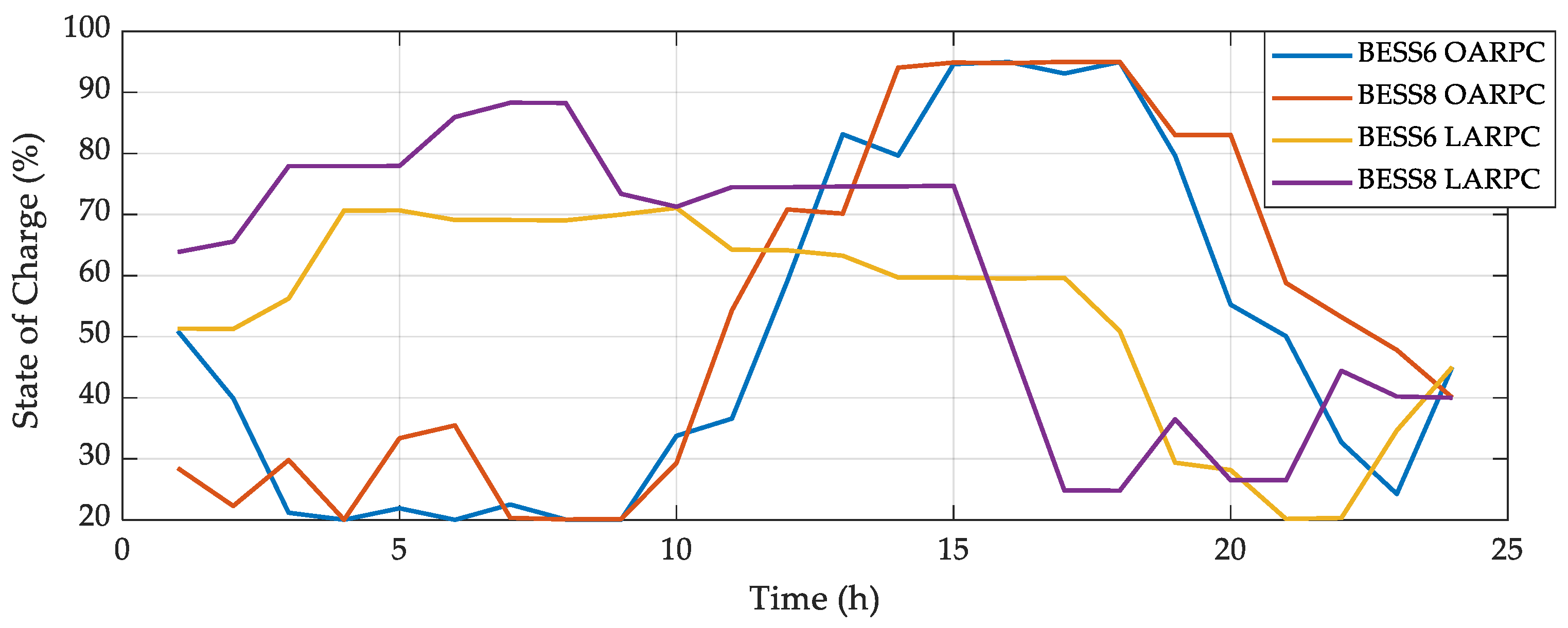
4.3.3. Local Active-Reactive Power Control for the Selected Day

This section presents the microgrid operation for the selected day under a Local Active-Reactive Power Control (LARPC) strategy in order to provide a reference scenario for evaluating the proposed two-stage OARPC impact upon the microgrid operation. The LARPC also consists of two stages, as the EVs and BESSs are scheduled during the first stage and the reactive power output for DGs, and CBs is determined in the second stage.

The active power control strategy within LARPC consists in applying the classical uniform EV scheduling scheme and then determining the BESS scheduling under the local load curve flattening strategy.

Firstly, the EVs are uniformly scheduled for charging in order to obtain a constant active power demand during the entire period while the EVs are parked at each charging station. For example, 25 EVs require two hours of charging each at the Office building connected at bus 3, between 7⁰⁰ and 17⁰⁰ h. During this period, there are five two-hour time intervals, therefore the EVs are divided into five groups of five EVs, each group starting to charge at 7⁰⁰, 9⁰⁰, 11⁰⁰, 13⁰⁰, and 15⁰⁰, resulting in a constant active power demand of 150 kW during the ten-hour interval. The second office building, connected at bus 6, is required to charge 30 EVs under identical conditions as the first office building, therefore the scheduling consists of charging the five groups of 6 EVs each using the aforementioned schedule. In a similar manner, the remaining 45 EVs that require charging are scheduled in order to assure a constant active power during the entire parking period.

Secondly, the two BESS are scheduled individually with the objective of flattening the load curve at their connection bus. In this regard, the proposed ISCA is applied for solving the two optimization problems. The SOC resulting from applying the local strategy is presented in Figure 10 in comparison with the SOC obtained by applying the OARPC. The results reveal that under the local strategy, both BESS are charging during the first part of the day, when the load demand is low in order to assure the load curve flattening, without considering the PVPP and WPP generation.

The second stage of LARPC consists in using the PVPPs inverters and the CBs to locally compensate for the reactive power demanded by the loads. For this purpose, the PVPP’s and CB’s reactive power output is set to fully compensate for the reactive power demanded by the local load, also considering their reactive power limits. The WPP is not included in this reactive power control strategy, as no local load is supplied from the WPP connection bus.

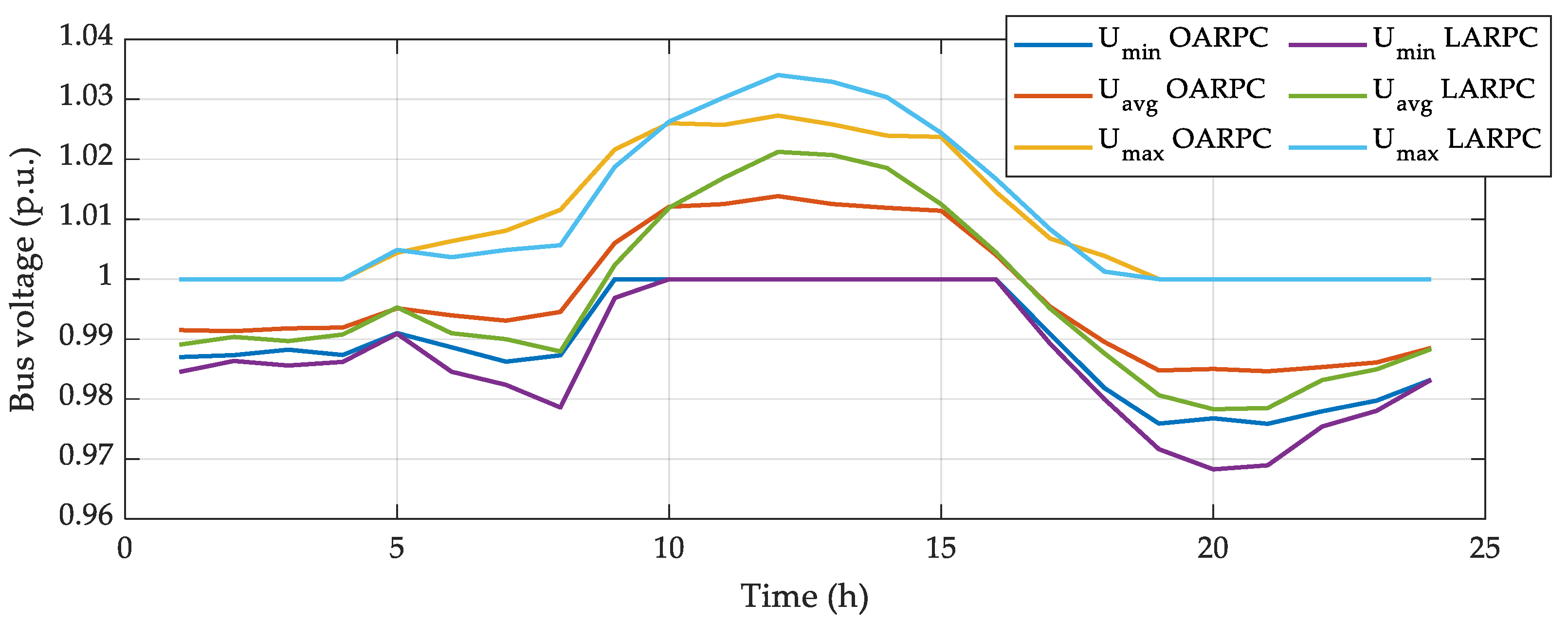
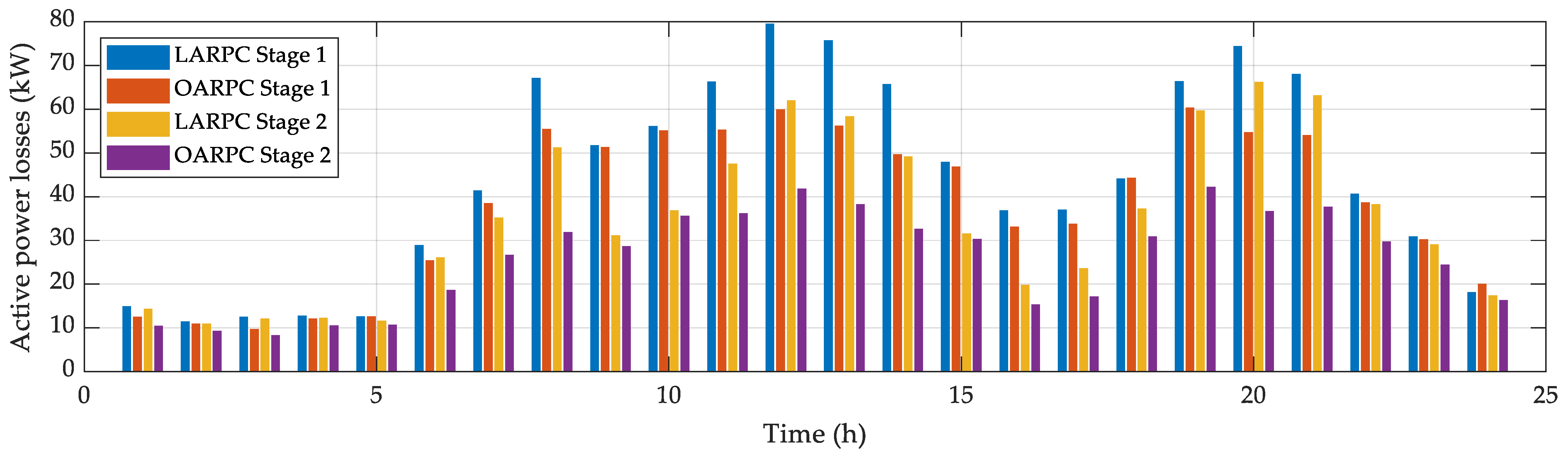
4.3.4. OARPC Impact upon Grid Operation for the Selected Day

In this section, the OARPC effect on the microgrid operation in terms of voltage profile, reactive power import, and active power losses is analysed. Firstly, the bus voltage profile for each microgrid bus, operating under the OARPC strategy, is presented in Figure 11, while a comparison between the hourly minimum, average and maximum bus voltage is presented in Figure 12.

The highest bus voltage profiles are observed at buses 11, 9, 8, and 2 with maximum values comprised between 1.027 p.u and 1.016 p.u and a minimum of 0.9881 p.u. This microgrid branch comprises the WPP at bus 11 which generates a significant amount of active and reactive power during the day, leading to increased bus voltage values including during the night and evening periods with no PVPP generation. The lowest voltage profile is observed for the other microgrid branch consisting of buses 3 to 7 and 10, with bus voltage values between 1.013 p.u. and 0.9758 p.u. However, it should be mentioned that during the day, the difference between the highest and lowest hourly bus voltage values is relatively reduced during the high PVPP generation period, with a minimum at 0.0077 p.u. and it increases at the 0.0243 p.u. during the morning and evening peak load demands periods when the PVPPs output is either reduced or zero.

A comparison between the central and local strategies’ impact on the microgrid bus voltage profile is presented in Figure 12 where the hourly minimum U_min, average U_avg and maximum U_max bus voltage values are presented for the local and central strategies. The results reveal that during the high PVPP generation interval between 9⁰⁰ and 16⁰⁰ the local strategy obtains higher average bus voltage values and equal minimum bus voltage values, while during the rest of the day the central strategy determines better U_avg and U_min values. A similar pattern is also observed for the U_max values, as under the local strategy the PVPPs are able to locally compensate the loads only during the midday period, while the only reactive power support for the rest of the day is provided by the two CBs. On the other hand, under the central strategy, the WPP provides significant reactive power support during the day. However, the differences between the bus voltage profiles determined by the two strategies are relatively reduced, with a maximum of 0.0087 p.u. during the selected day.

The microgrid reactive power import Q_sl is presented in Figure 13 for both stages of the central and local strategies. The results reveal that the central strategy successfully utilizes the reactive power support provided by the PVPPs, WPP, and CBs for reducing the reactive power import during the morning peak (5⁰⁰–9⁰⁰) from 682–1305 kVAr to 5–145 kVAr and during the evening peak (18⁰⁰–22⁰⁰) from 727–1172 kVAr to 60–279 kVAr.

After applying the first stage of both strategies, the microgrid would demand 1092 kVAr–1182 kVAr from the upstream network during the midday period. However, the significant reactive power support provided PVPPs under the second stage of the local strategy resulted in a reactive power export between 70 and 160 kVAr. During the rest of the day, the local strategy mainly relies on the CBs for reactive power support, therefore a limited reduction of Q_sl is observed. By comparison, the OARPC determines a constant reactive power export of 46 kVAr, while during the rest of the day insignificant reactive power exchanges are observed.

The local strategy is considered a reference for evaluating the OARPC performance, as classical scheduling methods are applied locally without any coordination between the different types of devices. During the first stage of the local strategy, EVs are scheduled independently of load demand and generation, while the BESS is scheduled only to flatten the load curve at the connection bus. By comparison, the first stage of the central strategy determines coordinated scheduling for all the EVs and both BESS, considering all loads and all distributed generators within the microgrid. Therefore, OARPC avoids charging EVs during the morning and evening load peaks or when the generation is at its lowest, while scheduling the maximum number of EVs during the maximum generation periods. Furthermore, both BESS are scheduled to charge during the highest generation period and supply active power to the microgrid during the low generation and high load demand periods. A comparison between the active power losses obtained by each stage of both strategies is presented in Figure 14. As the results reveal, after the first stage, OARPC obtains lower active power losses than the local strategy during the entire day. The largest active power loss reduction under the OARPC strategy, of approximately 25% relative to the local control scheme is observed during the 11⁰⁰–14⁰⁰ and 19⁰⁰–20⁰⁰ periods. During the entire day, the active energy losses are reduced by 13.2%, from 1061.8 kWh under the local strategy to 921.4 kWh under the OARPC strategy.

The second stage of the local strategy consists in using reactive power provided by the PVPPs and CBs for assuring local load compensation, while the WPP is not included as no local load is supplied from its connection bus. On the other hand, the central strategy utilizes all PVPPs, CBs, and the WPP reactive power support in order to minimize the total active power losses by considering all loads within the microgrid. Consequently, the active power losses are reduced by the OARPC during the entire day, with the largest differences of 29.3%–44.6% observed during the evening peak (18⁰⁰–21⁰⁰) and 37.3% during the 7⁰⁰–8⁰⁰ interval in the morning peak. The total daily active energy losses are reduced by OARPC from 845.5 kWh to 621.0 kWh, which represents a 26.55% reduction relative to the local strategy second-stage values.

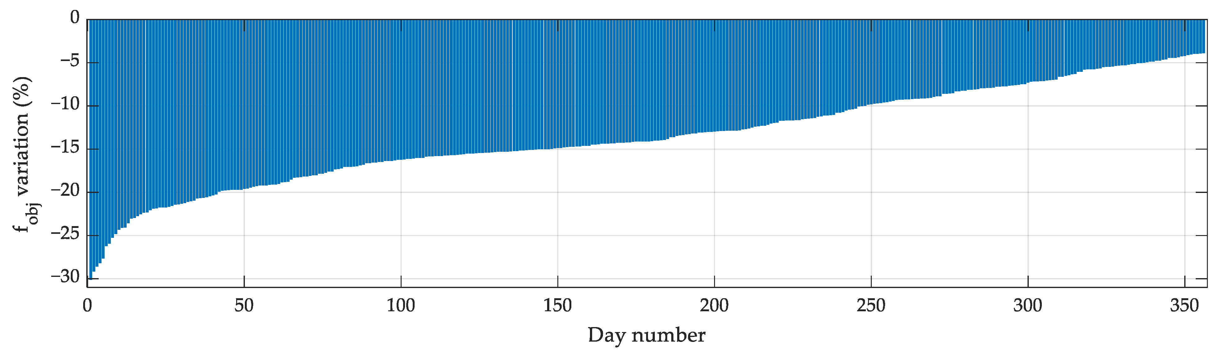
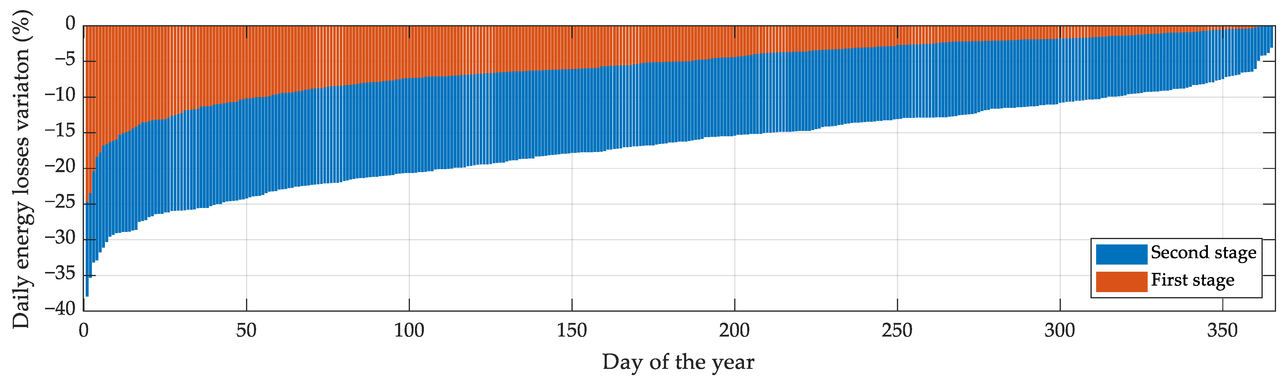
4.3.5. Overview of the OARPC Microgrid Operation Impact for One-Year Period

The results obtained by solving the OARPC problem using the ISCA during the one-year period are presented in this section, considering the results obtained by the LARPC strategy as a reference.

The daily energy loss variation between each stage of the OARPC and LARPC strategies is presented in Figure 15, expressed in percentage. The results reveal that the first OARPC stage reduces the daily energy losses by more than 20% during three days of the year, while for another six days the decrease is less than 0.2%. Furthermore, a 10% improvement in active energy losses is obtained for 53 days, while a 5% reduction is observed for 182 days. After the second stage, the OARPC reduces the active power losses between 3.1% and 37.9%, in comparison to the second LARPC stage. As the results show a 20% decrease is obtained for 113 days, while a 10% improvement is obtained for 275 days during the year. Finally, an annual average active energy loss reduction of 4.4%% is obtained after the first stage OARPC stage, and 15.2% after the second OARPC stage in comparison with the local strategy.

5. Conclusions

Considering the recent developments in the energy industry, namely the penetration of renewable energy sources at both utility-scale and end-user scale, in addition to the significant advances in electrification of the transportation sector, the necessity of implementing the microgrid concept considerably increased. Grid operators are challenged by the integration of electric vehicles and renewable energy sources, as the grid infrastructure was not developed to deal with their intermittent nature. In order to maintain the safety of the power supply, different controllable devices were introduced, with battery energy storage systems being the most promising solution. However, as the number of controllable devices increases, the main solution for achieving the integration of highly renewable energy sources and electric vehicles, while maintaining the safety of the power supply is represented by the implementation of coordinated control strategies.

In this regard, an Optimal Active-Reactive Power Coordination problem is formulated in this paper, for minimizing the microgrid daily active energy losses, considering the high penetration of photovoltaics and wind energy, electric vehicles, and battery energy storage systems. Given its increased complexity, the OARPC problem is solved in two successive stages by first determining the optimal scheduling for the EVs and BESSs and then the optimal reactive power of DGs and CBs.

An Improved Sine-Cosine Algorithm is proposed in this paper in order to handle the increased computational effort of solving the complex OARPC problem. The performance analysis conducted between the proposed algorithm and the original SCA, demonstrated that the ISCA obtains a significant performance increase for solving the OARPC problem.

The case study presented in this paper is conducted on a microgrid inspired by the CIGRE Medium Voltage benchmark network, including renewable energy sources, storage devices, electric vehicles, and capacitor banks, with the objective of evaluating the model’s capability to identify the optimal active-reactive scheduling for multiple generation and consumption scenarios. The proposed OARPC methodology was compared to a local control strategy, as well, to emphasize the benefits of centralized control schemes upon microgrid operation, as the results showed significant improvement in energy losses reduction.

Future works may involve the integration of economic aspects, thus modelling the interaction between the utility grid, microgrid operator, and end-user.

References

1. Schmidt, M.; Staudt, P.; Weinhardt, C. Decision support and strategies for the electrification of commercial fleets. Transp. Res. Part D Transp. Environ. 2021, 97, 102894. [Google Scholar] [CrossRef]
2. Al-Shetwi, A.Q.; Hannan, M.; Jern, K.P.; Mansur, M.; Mahlia, T. Grid-connected renewable energy sources: Review of the recent integration requirements and control methods. J. Clean. Prod. 2020, 253, 119831. [Google Scholar] [CrossRef]
3. Singh, J.; Tiwari, R. Probabilistic modeling and analysis of aggregated electric vehicle charging station load on distribution system. In Proceedings of the 14th IEEE India Council International Conference (INDICON), Roorkee, India, 16–17 December 2017. [Google Scholar]
4. Mastoi, M.S.; Zhuang, S.; Munir, H.M.; Haris, M.; Hassan, M.; Usman, M.; Bukhari, S.S.H.; Ro, J.S. An in-depth analysis of electric vehicle charging station infrastructure, policy implications, and future trends. Energy Rep. 2022, 8, 11504–11529. [Google Scholar] [CrossRef]
5. Sun, B.; Huang, Z.; Tan, X.; Tsang, D.H. Optimal scheduling for electric vehicle charging with discrete charging levels in distribution grid. IEEE Trans. Smart Grid 2018, 9, 624–634. [Google Scholar] [CrossRef]
6. Yilmaz, M.; Krein, P.T. Review of battery charger topologies, charging power levels, and infrastructure for plug-in electric and hybrid vehicles. IEEE Trans. Power Electron. 2013, 28, 2151–2169. [Google Scholar] [CrossRef]
7. Shafiee, S.; Fotuhi-Firuzabad, M.; Rastegar, M. Investigating the impacts of plug-in hybrid electric vehicles on power distribution systems. IEEE Trans. Smart Grid 2013, 4, 1351–1360. [Google Scholar] [CrossRef]
8. Dulău, L.I.; Bică, D. Effects of electric vehicles on power networks. Procedia Manuf. 2020, 46, 370–377. [Google Scholar] [CrossRef]
9. Aghajan-Eshkevari, S.; Azad, S.; Nazari-Heris, M.; Ameli, M.T.; Asadi, S. Charging and discharging of electric vehicles in power systems: An updated and detailed review of methods, control structures, objectives, and optimization methodologies. Sustainability 2022, 14, 2137. [Google Scholar] [CrossRef]
10. Wu, Y.; Wang, Z.; Huangfu, Y.; Ravey, A.; Chrenko, D.; Gao, F. Hierarchical operation of electric vehicle charging station in smart grid integration applications—An overview. Int. J. Electr. Power Energy Syst. 2022, 139, 108005. [Google Scholar] [CrossRef]
11. Xu, S.; Yan, Z.; Feng, D.; Zhao, X. Decentralized charging control strategy of the electric vehicle aggregator based on augmented Lagrangian method. Int. J. Electr. Power Energy Syst. 2019, 104, 673–679. [Google Scholar] [CrossRef]
12. Cheng, S.; Feng, Y.; Wang, X. Application of lagrange relaxation to decentralized optimization of dispatching a charging station for electric vehicles. Electronics 2019, 8, 288. [Google Scholar] [CrossRef] [Green Version]
13. Paudel, A.; Hussain, S.A.; Sadiq, R.; Zareipour, H.; Hewage, K. Decentralized cooperative approach for electric vehicle charging. J. Clean. Prod. 2022, 364, 132590. [Google Scholar] [CrossRef]
14. Jain, A.; Karimi-Ghartemani, M. Mitigating adverse impacts of increased electric vehicle charging on distribution transformers. Energies 2022, 15, 9023. [Google Scholar] [CrossRef]
15. Aygun, A.I.; Kamalasadan, S. Centralized charging approach to manage electric vehicle fleets for balanced grid. In Proceedings of the 2022 IEEE International Conference on Power Electronics, Smart Grid, and Renewable Energy (PESGRE), Trivandrum, India, 2–5 January 2022. [Google Scholar]
16. Chen, H.; Hu, Z.; Zhang, H.; Luo, H. Coordinated charging and discharging strategies for plug-in electric bus fast charging station with energy storage system. IET Gener. Transm. Distrib. 2018, 12, 2019–2028. [Google Scholar] [CrossRef] [Green Version]
17. Kucevic, D.; Englberger, S.; Sharma, A.; Trivedi, A.; Tepe, B.; Schachler, B.; Hesse, H.; Srinivasan, D.; Jossen, A. Reducing grid peak load through the coordinated control of battery energy storage systems located at electric vehicle charging parks. Appl. Energy 2021, 295, 116936. [Google Scholar] [CrossRef]
18. Jiang, W.; Zhen, Y. A real-time EV charging scheduling for parking lots with PV system and energy store system. IEEE Access 2019, 7, 86184–86193. [Google Scholar] [CrossRef]
19. Nour, M.; Ali, A.; Farkas, C. Mitigation of electric vehicles charging impacts on distribution network with photovoltaic generation. In Proceedings of the 2019 International Conference on Innovative Trends in Computer Engineering (ITCE), Aswan, Egypt, 2–4 February 2019. [Google Scholar]
20. Li, S.; Zhang, T.; Liu, X.; Xue, Z.; Liu, X. Performance investigation of a grid-connected system integrated photovoltaic, battery storage and electric vehicles: A case study for gymnasium building. Energy Build. 2022, 270, 112255. [Google Scholar] [CrossRef]
21. Dai, Q.; Liu, J.; Wei, Q. Optimal photovoltaic/battery energy storage/electric vehicle charging station design based on multi-agent particle swarm optimization algorithm. Sustainability 2019, 11, 1973. [Google Scholar] [CrossRef] [Green Version]
22. Trivedi, R.; Patra, S.; Sidqi, Y.; Bowler, B.; Zimmermann, F.; Deconinck, G.; Papaemmanouil, A.; Khadem, S. Community-based microgrids: Literature review and pathways to decarbonise the local electricity network. Energies 2022, 15, 918. [Google Scholar] [CrossRef]
23. Morstyn, T.; Hredzak, B.; Agelidis, V.G. Control strategies for microgrids with distributed energy storage systems: An overview. IEEE Trans. Smart Grid 2018, 9, 3652–3666. [Google Scholar] [CrossRef]
24. Jiang, X.; Wang, J.; Han, Y.; Zhao, Q. Coordination dispatch of electric vehicles charging/discharging and renewable energy resources power in microgrid. Procedia Comput. Sci. 2017, 107, 157–163. [Google Scholar] [CrossRef]
25. Chang, S.; Niu, Y.; Jia, T. Coordinate scheduling of electric vehicles in charging stations supported by microgrids. Electr. Power Syst. Res. 2021, 199, 107418. [Google Scholar] [CrossRef]
26. Conseil International des Grands Réseaux Électriques; Comité D’études C6. Benchmark Systems for Network Integration of Renewable and Distributed Energy Resources; CIGRÉ: Paris, France, 2014; ISBN 978-2-85873-270-8. [Google Scholar]
27. Mirjalili, S. SCA: A sine cosine algorithm for solving optimization problems. Knowl. Based Syst. 2016, 96, 120–133. [Google Scholar] [CrossRef]
28. Saddique, M.S.; Habib, S.; Haroon, S.S.; Bhatti, A.R.; Amin, S.; Ahmed, E.M. Optimal solution of reactive power dispatch in transmission system to minimize power losses using sine-cosine algorithm. IEEE Access 2022, 10, 20223–20239. [Google Scholar] [CrossRef]
29. Liu, S.; Feng, Z.-K.; Niu, W.-J.; Zhang, H.-R.; Song, Z.-G. Peak operation problem solving for hydropower reservoirs by elite-guide sine cosine algorithm with gaussian local search and random mutation. Energies 2019, 12, 2189. [Google Scholar] [CrossRef] [Green Version]
30. Attia, A.-F.; El Sehiemy, R.A.; Hasanien, H.M. Optimal power flow solution in power systems using a novel Sine-Cosine algorithm. Int. J. Electr. Power Energy Syst. 2018, 99, 331–343. [Google Scholar] [CrossRef]
31. Abdel-Mawgoud, H.; Fathy, A.; Kamel, S. An effective hybrid approach based on arithmetic optimization algorithm and sine cosine algorithm for integrating battery energy storage system into distribution networks. J. Energy Storage 2022, 49, 104154. [Google Scholar] [CrossRef]
32. Jouhari, H.; Lei, D.; Al-qaness, M.A.A.; Abd Elaziz, M.; Ewees, A.A.; Farouk, O. Sine-cosine algorithm to enhance simulated annealing for unrelated parallel machine scheduling with setup times. Mathematics 2019, 7, 1120. [Google Scholar] [CrossRef] [Green Version]
33. Gabis, A.B.; Meraihi, Y.; Mirjalili, S.; Ramdane-Cherif, A. A comprehensive survey of sine cosine algorithm: Variants and applications. Artif. Intell. Rev. 2021, 54, 5469–5540. [Google Scholar] [CrossRef]
34. Shaheen, A.M.; Spea, S.R.; Farrag, S.M.; Abido, M.A. A review of meta-heuristic algorithms for reactive power planning problem. Ain Shams Eng. J. 2018, 9, 215–231. [Google Scholar] [CrossRef]
35. Rupa, J.A.M.; Ganesh, S. Power flow analysis for radial distribution system using backward/forward sweep method. Int. J. Electr. Comput. Electron. Commun. Eng. 2014, 10, 1540–1544. [Google Scholar]
36. Eremia, M. Electric Power Systems—Electric Networks; Publishing House of the Romanian Academy: Bucharest, Romania, 2006; pp. 509–520. [Google Scholar]
37. Simulated Load Profiles for DOE Commercial Reference Buildings (17 Years Using NSRD Data), U.S. Department of Energy. Available online: https://openei.org/datasets/dataset/simulated-load-profiles-17year-doe-commercial-reference-buildings (accessed on 6 November 2022).
38. Pfenninger, S.; Staffell, I. Long-term patterns of European PV output using 30 years of validated hourly reanalysis and satellite data. Energy 2016, 114, 1251–1265. [Google Scholar] [CrossRef] [Green Version]
39. Staffel, I.; Pfenninger, S. Using bias-corrected reanalysis to simulate current and future wind power output. Energy 2016, 114, 1224–1239. [Google Scholar] [CrossRef]
40. Available online: https://www.renewables.ninja/ (accessed on 6 November 2022).
Figure 1. Two-stage Active-Reactive Power Coordinated Optimization Flowchart.
Mathematics 11 00045 g001
Figure 2. One-line diagram for the considered microgrid.
Mathematics 11 00045 g002
Figure 3. Performance comparison between the ISCA and SCA during each day of the year.
Mathematics 11 00045 g003
Figure 4. Load and generation curves for the selected day 29th of March.
Mathematics 11 00045 g004
Figure 5. The EV scheduling determined after the first stage of OARPC for the selected day.
Mathematics 11 00045 g005
Figure 6. The optimal scheduling for the BESS connected at (a) bus 6 and (b) bus 8, determined after the first stage of OARPC for the selected day.
Mathematics 11 00045 g006
Figure 7. Microgrid active power scheduling resulted after the first OARPC stage for the selected day.
Mathematics 11 00045 g007
Figure 8. Reactive power output for the distributed sources for the selected day.
Mathematics 11 00045 g008
Figure 9. Operational step for the capacitor banks for the selected day.
Mathematics 11 00045 g009
Figure 10. BESS scheduling under the LARPC and OARPC strategies for the selected day.
Mathematics 11 00045 g010
Figure 11. Microgrid hourly bus voltage profile for the selected day, under the OARPC.
Mathematics 11 00045 g011
Figure 12. Hourly minimum, average and maximum voltage profiles comparison between OARPC and LARPC.
Mathematics 11 00045 g012
Figure 13. Reactive power import profile comparison for both stages of OARPC and LARPC.
Mathematics 11 00045 g013
Figure 14. Hourly active power losses profile comparison for both stages of OARPC and LARPC.
Mathematics 11 00045 g014
Figure 15. Daily energy losses variation between each stage of LARPC and OARPC strategies.
Mathematics 11 00045 g015