Abstract
Empirical evidence suggests that financial risk has a heavy-tailed profile. Motivated by recent advances in the generalized quantile risk measure, we propose the tail value-at-risk (TVaR)-based expectile, which can capture the tail risk compared with the classic expectile. In addition to showing that the risk measure is well-defined, the properties of TVaR-based expectiles as risk measures were also studied. In particular, we give the equivalent characterization of the coherency. For extreme risks, usually modeled by a regularly varying survival function, the asymptotic expansion of a TVaR-based expectile (with respect to quantiles) was studied. In addition, motivated by recent advances in distributionally robust optimization in portfolio selections, we give the closed-form of the worst-case TVaR-based expectile based on moment information. Based on this closed form of the worst-case TVaR-based expectile, the distributionally robust portfolio selection problem is reduced to a convex quadratic program. Numerical results are also presented to illustrate the performance of the new risk measure compared with classic risk measures, such as tail value-at-risk-based expectiles.
Keywords:
expectile; coherent risk measure; worst-case risk measure; distributionally robust optimization; heavy-tailed risks MSC:
91G70
1. Introduction
A risk measure involves mapping , where is a set of loss random variables or risks. Risk measures were well used in solvency risk management to determine the required capital for risks. Among others, expectile, introduced in Newey and Powell [1] as the minimizers of asymmetric quadratic loss functions in the context of regression, is one of the most important risk measures in risk management. For a risk X with , the expectile of X at a confidence level , written as , is defined as the unique minimizer of the following problem:
where . Equivalently, is the unique solution to the equation
Note that the above definition (1) is well-defined for any risk X with finite mean.
Bellini et al. [2] showed that the expectile for is a coherent risk measure (whose definition, as introduced by Artzner et al. [3], will be given later). Starting from this seminal paper in risk management, expectiles are gaining popularity in econometric literature studies and actuarial science (e.g., Bellini et al. [2] and Cai and Weng [4]). An expectile has the property of elicitability, which is an essential and desirable property in backtesting and forecasting (e.g., Gneiting [5] and Kratz et al. [6]). In addition, Ziegel [7] showed that the expectile is the only coherent risk measure class that has elicitability. See Bellini et al. [2], Ziegel [7], Embrechts et al. [8], and the references therein for more discussions on the properties of expectiles.
From the point view of solvency risk management, based on the definition of (1), if x is the required capital for the risk X, then and are viewed as the shortfall risk and the over-required capital risk, respectively. For , we can rewrite (1) as , . With serving as the required capital, the ratio of the expected shortfall risk to the expected over-required capital risk is . Obviously, it is desired that the expected shortfall risk is not larger than the expected over-required capital risk or that the ratio satisfies or equivalent , which is a necessary and sufficient condition for the expectile to be a coherent risk measure.
As argued by Mao and Cai [9], the shortfall risk and the over-required capital risk in the expectile definition are evaluated under the probability measure or the distribution of X. A decision-maker may have different attitudes toward the different outcomes of risks, and it is reasonable to employ more conservative risk measures than expectations to evaluate the risks. The tail value-at-risk (TVaR), the expected shortfall (ES), and the conditional VaR (CVaR) of X at a confidence level , defined as
are other important examples of coherent risk measures used in finance and insurance risk management, where is the left-continuous inverse of , defined by for . One can verify that for any and it reduces to the expectation when , which is a natural alternative conservative risk measure compared to the expectation of evaluating the risk. In this paper, we intend to employ TVaR instead of the expectation to evaluate the two risks in (1) and require the ratio to be equal to a given confidence level in which we generalize the definition of the classic expectile. The new risk measure is called the TVaR-based expectile.
In this paper, we first show that the TVaR-based expectile is well-defined, and we study its basic properties as risk measures. In particular, we give the equivalent characterization of the TVaR-based expectile being a coherent risk measure. As a generalization of the expectile, the TVaR-based expectile does not admit a closed form, which makes the estimation of the risk measure difficult. When the prudentiality level is close to 1, a preliminary step to the estimation involves the obtention of asymptotic expansions for the target risk measure. Such expansions allow quantifying bias terms and are fundamental in the derivation of asymptotic normality results for estimators at extreme levels, see, e.g., Cai et al. [10], Daouia et al. [11], and Zhao et al. [12]. Such asymptotic expansions can lead to better understanding of the risk measures and plug-in estimators at extreme levels (Daouia et al. [11]), and are very useful in practice as there is empirical evidence that financial risks have the properties of heavy tails. In this paper, we study the asymptotic expansions of TVaR-based expectiles for heavy-tailed risks with confidence levels close to 1. The results obtained in this paper recover the asymptotic expansions of the expectile given by Mao et al. [13].
The work of Delage and Ye [14] involves distributionally robust optimization (DRO) and has been recognized as the diagram in modeling distribution uncertainty. Motivated by recent advances in DRO in risk management (Blanchet et al. [15] and Li [16]), we studied the worst-case TVaR-based expectile based on moment information, which recovers the worst-case expectile. Based on this closed form of the worst-case TVaR-based expectile, we reduce the distributionally robust portfolio selection problem to a convex quadratic program. Numerical results are also presented to illustrate the performance of the new risk measures compared with classic risk measures, such as tail value-at-risk-based expectiles.
Throughout the paper, let be an atomless probability space, where is a set of possible states of nature and is -algebra on . Let be the spaces of all random variables and the spaces of all integrable random variables on , respectively, i.e., and . For a random variable , we denote by the cumulative distribution function (cdf) of X under the probability , i.e., , .
2. TVaR-Based Expectile
In this section, we present the formal definition of the TVaR-based expectile and study its properties as risk measures. We first give an auxiliary lemma, which guarantees that the definition of the TVaR-based expectile is well-defined.
Lemma 1.
For , , the equation of x:
has a unique solution, which also equals the unique solution to
where F is the distribution function of X.
Proof.
We first show that for and , it holds that
and
where F is the distribution function of X. Note that
Note that . We have
where the last equality follows from . We next consider two cases. If , then for and, thus,
For , then
Now, we introduce the TVaR-based risk measure of the expectile as follows.
Definition 1.
For a risk X, , and ,the TVaR-based expectile of X, denoted by , is the unique solution to the equation
When , then reduces to the classic expectile with level . In particular, we identify the following two special classes of TVaR-based expectiles.
- (i)
- If , i.e., the decision-maker has the same risk attitude to the shortfall risk and the over-required capital risk , and he/she uses the same TVaR to evaluate the two risks, in this case, the TVaR-based expectile of X, denoted by , is the unique solution to the equation
- (ii)
- If , , i.e., the decision maker is risk neutral to the shortfall risk and is risk averse to the over-required capital risk , and he/she uses the expectation and TVaR to evaluate the two risks, respectively, in this case, the TVaR-based expectile of X, denoted by , is the unique solution to the equation
By changing the parameters in the definition of the TVaR-based expectile, we can flexibly obtain different risk measures based on the purpose of risk evaluation. In the next subsection, we will study the properties of TVaR-based expectiles as risk measures.
2.1. Basic Properties
We next study the basic properties of the TVaR-based expectile introduced in Definition 1 as a risk measure. We list some desired properties of the risk measures as follows.
- (P1)
- Monotonicity: for all , such that is almost surely (a.s.).
- (P2)
- Translation invariance: for all and all .
- (P3)
- Positive homogeneity: for all and all .
- (P4)
- Subadditivity: for all .
It is well-known that a risk measure satisfying the above four properties is called a coherent risk measure, which is introduced by Artzner et al. [3].
Proposition 1.
For , let be defined by (7). We have the following result.
- (i)
- satisfies (P1) monotonicity, (P2) translation-invariance, and (P3) positive homogeneity.
- (ii)
- satisfies (P4) subadditivity if and only if and .
- (iii)
- increases in α and and decreases in .
- (iv)
- .
Proof.
- (i)
- The results follow from standard manipulation based on the definition (7).
- (ii)
- The necessary and sufficient conditions follow directly from Theorem 3.2 of Mao and Cai [9].
- (iii)
- The result can be verified directly based on (3).
- (iv)
- Note that for any , and and, thus, and Therefore, by the definition of , we haveand, thus, . This completes the proof. □
By Proposition 1, we immediately obtain the following result.
Corollary 1.
For , the TVaR-based expectile is a coherent risk measure if and only if and . In this case, the TVaR-based expectile reduces to the expectile at level α.
2.2. Asymptotic Expansion of TVaR-Based Expectile for Extreme Risks
We investigate the asymptotic properties of defined by (7) for extreme risks. We first view as a fixed weight on the shortfall risk and let in the definition of . In this case, we denote that , i.e., is the unique solution to the following equation
We study the asymptotic properties of when the confidence level converges to 1.
We first recall the definition of regular variation, which is an essential concept in defining the heavy-tailed risks. A function h is said to be regularly varying at point , denoted as , , if
For a random variable X, let be its cumulative distribution function. X is said to be regularly varying at both tails, denoted as , , if and . Here, and are called the indexes of regular variations. To state the results, let denote the quantile of X at level , defined by
where F is the distribution of X.
Proposition 2.
Let X be a random variable, such that it regularly varies at both tails with indexes and defined by the solution to (10). Then we have if ,
and if ,
Proof.
We only show the case that is the proof for and is similar by taking . When , we have , then , which is larger than . Hence, we have as the solution to
where
If , then the equation is
and the solution is . It is well-known that
Hence, we have . If , then we have for close to 1, and, thus,
If , then is the solution to
that is,
By Proposition 1.1 of Zhu [17] or Mao et al. [18], we have
Substituting this into (12) yields
Combining this with (11), we complete the proof. □
Remark 1.
- (i)
- In general, we could not obtain similar asymptotic results for the case . The reason is that even if , we may have converging to ∞ or 0 as . Let X be a symmetric distribution about and . Then .
- (ii)
- From Proposition 2, we have , which means the right tail is heavier than the left tail of X, then the is asymptotically determined by the right tail and is asymptotic equivalent to , multiplied by some constant. In contrast, if , which means the right-tail is lighter than the left tail of X, then the is asymptotically determined by the left tail and is asymptotic equivalent to , multiplied by some constant.
In the following proposition, we investigate the asymptotic properties of as goes to 1.
Proposition 3.
Let X be a random variable with the survival function , such that , and are defined by the solution to (10), . Then we have
Proof.
If , then reduces to the classic expectile . The asymptotics result in (14) reducing to
It is worth mentioning that this recovers the asymptotic expansion of the classic expectile in Mao et al. [13].
3. Distributionally Robust Optimization with the TVaR-Based Expectile
3.1. Worst-Case TVaR-Based Expectile
Motivated by recent advances in distributionally robust optimization (DRO), in this section, we study the worst-case TVaR-based expectile with respect to the moment constraint. DRO has arisen as a modeling paradigm for addressing the issue of distributional ambiguity in risk management (see, e.g., Delage and Ye [14]). The power of DRO lies in its flexibility in characterizing one’s (partial) knowledge of the distribution through specifying an ambiguity set. In particular, one common way of defining the ambiguity set is by specifying the moments of the distribution, i.e., we confine the possible distributions to the following ambiguity set
where and represent the mean and variance of X, respectively, under the constraint that X has the distribution F.
One special case of the TVaR-based expectile of X, denoted by , is the unique solution to the equation
We study the worst-case TVaR-based expectile given the expectation and variance . That is, we aim to find
where is the random variable with the distribution F. Note that satisfies the translation–invariance and positive homogeneity, i.e.,
Then . It suffices to investigate the special case that and . To show our main result, we need the following lemmas.
Lemma 2.
Let ρ be a risk measure satisfying translation–invariance and positive homogeneity and be the worst-case of ρ. If , then we have as increasing in μ and σ. Hence,
where is the set of all possible distributions of X, such that it has a mean no larger than μ and variance no larger than .
Lemma 3.
Let be the TVaR-based expectile of X defined by (7). Then .
Proof.
It suffices to show the case for . Consider a random variable given by
It is obvious that and . Letting , one can verify that goes to 0. To see it, suppose that for some . Then there exists , such that for , and in this case, . Denote
Then
Note that is a decreasing function in x and is the solution to . It then follows that for . That is, for , which yields a contradiction. Hence, this completes the proof. □
Combining Lemmas 2 and 3, we have that is increasing in and and, hence,
Remark 2.
Note that (7) can be rewritten as
If , it is obvious that and , which implies that for any random variable X. Hence, by Lemma 3, we have . Therefore, in the following, we only consider the case that .
Lemma 4.
Let be the TVaR-based expectile of X defined by (7). Then the worst-case distribution is a bivariate distribution. Specifically, we have
where is the set of all bivariate distributions in .
Proof.
By Lemmas 2 and 3, it suffices to show that for any distribution in , we can find a bivariate distribution in , such that its value of risk measure is no less than that of the original distribution. Let be a random variable with distribution and . Define
It is obvious that and , i.e., the distribution of belongs to . Note that and, thus, (let X and Y be two random variables X is said to be smaller than Y in increasing convex order, denoted by , if for any increasing convex function . X is said to be smaller than Y in convex order, denoted by , if and .), which implies
Moreover, note that . Then we have
This implies . Hence, we complete the proof. □
By Lemma 4, we only need to find the worst-case distribution in the set . Now we are ready to show the main result.
Theorem 1.
Proof .
Without loss of generality, we assume and . Then
We next calculate for for the following two cases. If , then satisfies the equation
and if , then satisfies the equation
That is,
Denote by and the two functions of the right-hand side of (17), respectively. By taking derivatives of with respect to , it is easy to see that takes its maximum value
and is increasing in and decreasing in . On the other hand, by taking derivatives of with respect to , one can verify that takes its maximum value
at
and is increasing in and decreasing in . Hence, by (17), the maximum value of could be attained at one of the points . We next consider the following three cases.
- (i)
- If , then one can find that confining on , takes its maximum value at point . On the other hand, note thatand , which imply Hence, we have in this case, . Then one can easily verify that . This implies that confining on , takes its maximum value at point and the corresponding maximum value is no less than . Therefore, takes its maximum value at .
- (ii)
- If , then one can verify that confining on , takes its maximum value at point , while confining on , takes its maximum value at point . Hence, to find the maximum value at the whole interval , we need to compare the values of at and . Note thatOne can verify that for ,is decreasing in . Hence, takes its minimum value at and its maximum value at . Note that . Moreover, we have , i.e., when ,where the first inequality follows from the mapping and is decreasing in . Then there exists a unique , such that it is the solution to the equation , i.e., , such that if , then and, thus, takes its maximum value at . If , then and, thus, takes its maximum value at .
- (iii)
- If , one can verify that and , i.e., . This implies that is increasing in and decreasing in . Therefore, takes its maximum value at .
Combining the above three cases, we complete the proof. □
Note that when , the TVaR-based expectile reduces to the classic expectile. By Li [16], we can show the following result for the expectile.
Corollary 2.
The worst-case expectile is given by
and the worst-case distribution F is given by
Proof.
For completeness, we give another direct proof. By Bellini et al. [2], we have the following dual representation,
where and with . Note that
By Lemma 2, we have
Note that in the above equation, the supremum is attained at the optimal . The corresponding distortion function has the left derivative function . Hence, the worst-case distribution F is given by
where is a constant. Then the result follows by taking variance as . This completes the proof. □
3.2. Application in the Portfolio Selection
In this subsection, we are interested in the following distributionally robust portfolio optimization problem under the mean-variance uncertainty set:
where
and represents the TVaR-based expectile of that is calculated under the constraint that the distribution of is F. This kind of distributionally robust portfolio optimization problem under different principles was recently studied by Sim et al. [19], Blanchet et al. [15] and the references therein. By Theorem 1 and the projection result on the moment-based ambiguity set by Chen et al. [20], we can reduce Problem (18). We first recall the projection result from Chen et al. [20]: For , it holds that
where
and
In the following theorem, we solve the inner problem of Problem (18) and give a equivalent optimization problem to Problem (18) in the sense that two problems have the same optimal solution.
Theorem 2.
4. Empirical Results
To demonstrate the viability and robustness of the proposed approach, a robust optimal portfolio strategy was determined using Python programming. A total of 10 stocks from diverse sectors of the Chinese stock market were selected to comprise the portfolio. The stock codes that make up the portfolio in the empirical study are shown in the Table 1 and is a 10-dimensional vector where represents the ith stock return for

Table 1.
The assets from the Chinese stock market.
We obtained the daily closing prices for these 485 stocks from cn.investing.com for the period from 1 January 2020 to 31 December 2021. The Table 2 shows key characteristics of the 10 stock returns, such as the mean, variance, and correlation coefficients.
Table 2.
Means, variance, and correlation coefficients of stock returns.
We present below the comparative models used in the empirical studies, mainly the classical portfolio model, the equally weighted portfolio model, and the portfolio model based on the risk measure CVaR. According to Harry Markowitz [21], the core idea of the traditional portfolio model is the strategy of minimizing variance to achieve the optimal weighting based on the presumption that the expected return is greater than the risk-free return. The equally weighted model is an equally weighted investment strategy in which the total capital is dynamically allocated equally to each asset in the portfolio. This is a simple but highly effective strategy. However, in the presence of large stocks with high volatility, many optimal strategies will be biased toward the investment strategy. The primary idea of the CVaR-based portfolio model is to determine the optimal weights based on the available data in order to minimize the CVaR under conditions of returns that are greater than predicted.
We obtain the worst-case TVaR-based expectile by setting various anticipated returns and inserting them into the theorem, where , and , respectively. The Figure 1 displays the worst-case efficiency bounds generated by the robust portfolio and classical portfolio models. Note that the classical portfolio model is based on the mean-variance model to compute the optimal weights to bring into Equation (19) in order to obtain the largest risk exposure achievable using the classical portfolio strategy.
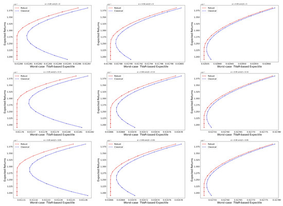
Figure 1.
The effective boundaries of the classical investment strategy and robust investment strategy based on the worst-case TVaR-based expectile.
Given the same desired return, the worst-case TVaR-based expectile of a robust portfolio strategy is less than the corresponding risk of a classical portfolio strategy. This is intuitive, as the objective of the robust model is to minimize the worst-case TVaR-based expectile. The following is an empirical examination of the performance of the robust portfolio model.
Using the first 30 days of stock data, and assuming an initial asset value of 1 and a sliding time window of 30 days, we determine the optimal weight vector for the various strategy models. Then, we utilize this weight vector for the following day’s investment and the return vector for that day to obtain the new asset value. Following this approach and advancing the data, we can finally obtain the cumulative returns for the various investment strategies from 2020 to 2022. The results are displayed in the Figure 2.
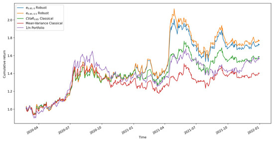
Figure 2.
Cumulative returns of optimal portfolio strategies under different strategies.
The general trend in cumulative return values indicates a minor decline in the market in early 2020 due to COVID-19. During the decline, the robust portfolio was much more stable than other investment strategies, experiencing smaller decreases than other strategies. Due to the well-controlled epidemic in China, the subsequent swift recovery of the Chinese economy, and the general outstanding performance of the stock market, the portfolio has steadily gained value, with the equal-weighted investment model demonstrating the highest returns.
Nevertheless, due to market volatility, the other investment strategies lost more than the robust investment strategy during the stock market decline in 2021; therefore, the final findings indicate that the robust portfolio has the best cumulative return, followed by the CVaR-based portfolio model and finally the equal-weighted model and the mean-variance model. As a result, the robust investment model performs admirably in terms of both its robustness and its cumulative returns.
5. Conclusions
In this paper, to better capture the tail risk, we propose a class of new risk measures called TVaR-based expectiles. The basic properties of risk measures, such as monotonicity, translation invariance, positive homogeneity, and subadditivity are studied. In particular, the equivalent characterization of coherency is given. For a better understanding of TVaR-based expectiles for extreme risks, asymptotic expansions with respect to quantiles were investigated. In addition, the closed-form of the worst-case TVaR-based expectile under the moment uncertainty set was obtained, and based on this closed-form, the distributionally robust portfolio selection problem with the principle of the TVaR-based expectile was reduced to a convex quadratic program. The empirical results for financial data were given to illustrate the performance of the new risk measure compared with the classic expectile and TVaR. Compared with the classic expectile, our TVaR-based expectiles employ more conservative risk measures than expectations to evaluate the risks and, thus, put more weight on the tail risk, which is more reasonable in practice.
Author Contributions
Conceptualization, H.C. and K.F.; methodology, K.F.; software, H.C.; validation, H.C. and K.F.; formal analysis, H.C.; investigation, H.C.; resources, H.C.; data curation, H.C.; writing—original draft preparation, K.F.; writing—review and editing, K.F.; visualization, H.C.; supervision, K.F.; project administration, K.F.; funding acquisition, K.F. All authors have read and agreed to the published version of the manuscript.
Funding
This research was funded by National Natural Science Foundation of China grant number 11971172.
Data Availability Statement
Publicly available datasets were analyzed in this study. This data can be found here: [cn.investing.com].
Acknowledgments
The authors thank the area editor, the associate editor, and the anonymous reviewer for their very careful reading of the paper and the many constructive comments, which helped us improve the quality of the paper.
Conflicts of Interest
The authors declare no conflict of interest.
References
- Newey, W.K.; Powell, J.L. Asymmetric least squares estimation and testing. Econometrica 1987, 55, 819–847. [Google Scholar] [CrossRef]
- Bellini, F.; Klar, B.; Müller, A.; Gianin, E.R. Generalized quantiles as risk measures. Insur. Math. Econ. 2014, 54, 41–48. [Google Scholar] [CrossRef]
- Artzner, P.; Delbaen, F.; Eber, J.-M.; Heath, D. Coherent measures of risk. Math. Financ. 1999, 9, 203–228. [Google Scholar] [CrossRef]
- Cai, J.; Weng, C. Optimal reinsurance with expectile. Scand. Actuar. J. 2016, 2016, 624–645. [Google Scholar] [CrossRef]
- Gneiting, T. Making and evaluating point forecasts. J. Am. Stat. Assoc. 2011, 106, 746–762. [Google Scholar] [CrossRef]
- Kratz, M.; Lok, Y.H.; McNeil, A. Multinomial VaR backtests: A simple implicit approach to backtesting expected shortfall. J. Bank. Financ. 2018, 88, 393–407. [Google Scholar] [CrossRef]
- Ziegel, J.F. Coherence and elicitability. Math. Financ. 2014, 26, 901–918. [Google Scholar] [CrossRef]
- Embrechts, P.; Mao, T.; Wang, Q.; Wang, R. Bayes risk, elicitability, and the Expected Shortfall. Math. Financ. 2021, 31, 1190–1217. [Google Scholar] [CrossRef]
- Mao, T.; Cai, J. Risk measures based on the behavioural economics theory. Financ. Stoch. 2018, 22, 367–393. [Google Scholar] [CrossRef]
- Cai, J.; Wang, Y.; Mao, T. Tail subadditivity of distortion risk measures and multivariate tail distortion risk measures. Insur. Math. Econ. 2017, 75, 105–116. [Google Scholar] [CrossRef]
- Daouia, A.; Girard, S.; Stupfler, G. Estimation of tail risk based on extreme expectiles. J. R. Statist. Soc. B 2018, 80 Pt 2, 263–292. [Google Scholar] [CrossRef]
- Zhao, Y.; Mao, T.; Yang, F. Estimation of the Haezendonck-Goovaerts risk measure for extreme risks. Scand. Actuar. J. 2021, 7, 599–622. [Google Scholar] [CrossRef]
- Mao, T.; Ng, K.; Hu, T. Asymptotic expansions of generalized quantiles and expectiles for extreme risks. Probab. Eng. Inform. Sci. 2015, 29, 309–327. [Google Scholar] [CrossRef]
- Delage, E.; Ye, Y. Distributionally robust optimization under moment uncertainty with application to data-driven problems. Oper. Res. 2010, 58, 595–612. [Google Scholar] [CrossRef]
- Blanchet, J.; Chen, L.; Zhou, X. Distributionally robust mean-variance portfolio selection with Wasserstein distances. Manag. Sci. 2022, 68, 6382–6410. [Google Scholar] [CrossRef]
- Li, Y.M. Closed-form solutions for worst-case law invariant risk measures with application to robust portfolio optimization. Oper. Res. 2018, 66, 1533–1541. [Google Scholar] [CrossRef]
- Zhu, L.; Li, H. Asymptotic analysis of multivariate tail conditional expectations. N. Am. Actuar. J. 2012, 16, 350–363. [Google Scholar] [CrossRef]
- Mao, T.; Lv, W.; Hu, T. Second-order expansions of the risk concentration based on CTE. Insur. Math. Econ. 2012, 51, 449–456. [Google Scholar] [CrossRef]
- Sim, M.; Zhao, L.; Zhou, M. Tractable Robust Supervised Learning Models. 2021. Available online: https://ssrn.com/abstract=3981205 (accessed on 9 December 2021).
- Chen, L.; He, S.; Zhang, S. Tight bounds for some risk measures with application to robust portfolio selection. Oper. Res. 2011, 59, 847–865. [Google Scholar] [CrossRef]
- Markowitz, H. Portfolio Selection. J. Financ. 1952, 7, 77–91. [Google Scholar]


Disclaimer/Publisher’s Note: The statements, opinions and data contained in all publications are solely those of the individual author(s) and contributor(s) and not of MDPI and/or the editor(s). MDPI and/or the editor(s) disclaim responsibility for any injury to people or property resulting from any ideas, methods, instructions or products referred to in the content. |
© 2022 by the authors. Licensee MDPI, Basel, Switzerland. This article is an open access article distributed under the terms and conditions of the Creative Commons Attribution (CC BY) license (https://creativecommons.org/licenses/by/4.0/).