Abstract
At present, a significant part of oil is extracted from difficult-to-develop reservoirs with low permeability. Hydraulic fracturing is one of the most important methods of production stimulation. Scientific articles do not describe the connections between the flow-rate in the well and the change in pressure in the hydraulic fracture or between the changing pressure in the well and the pressure in the hydraulic fracture, except in some cases of constant fluid-flow in the well and constant production. We obtained both the exact analytical solutions and the simple approximate solutions which describe the connection between the well-fluid flow-rate and the pressure evolution in a fracture. The work has also solved the inverse problem: how to determine the parameters of a hydraulic fracture, knowing the change in well flow-rate and the change in fluid-flow. The results show good comparison with practical data.
Keywords:
mathematical modeling; oil reservoir; integro-differential equation; hydraulic fracture; pressure evolution; flow-rate MSC:
76-10
1. Introduction
Hydraulic fracturing is one of the main methods for increasing hydrocarbon production. Fractures that appear or that widen already existing fractures during the injection of proppant fluid, connecting with each other, became conductors of oil or water. Fractures connect the well to remote zones of the formation, expanding the reachable area and facilitating the transport of oil to the well during fluid recovery or increasing fluid flow from the well during injection. The created fractures are fixed with a proppant in order to prevent their closing after the fluid supply is stopped under high pressure. Modeling the process of hydraulic fracturing and fluid filtration in the vicinity of a well with hydraulic fracturing is a complicated process. The development of computer technology makes it possible to improve models. However, the current level does not allow abandoning an approximate description of processes or neglecting any of them. There are many works devoted to various methods of creating fractures in oil reservoirs (see [1]). Various fracture-geometry models are suggested. The best known models are KGD (Khristianovich–Geertsma–de Klerk geometry) [2,3] and PKN (Perkins–Kern–Nordgren geometry) [4,5]. Different hydraulic fracture models give well-consistent results.
In [6], Gringarten and Ramey Jr., and the article by Cinco L., et al. [7] show different periods of filtration, in accordance with the nature of the change in bottom hole pressure, and a system of differential equations is offered, describing fluid filtration in the hydraulic fracture and the formation around the fracture. The operation of a well with a vertical hydraulic fracture in constant flow or constant pressure modes at the well is described in [8,9,10,11]. The methods used in practice to describe filtration flows around wells are focused on steady-state operation modes or use less accurate models, and use numerical solution methods requiring a large number of calculations.
In this paper, we have solved the problem of pressure distribution in a vertical hydraulic fracture under various well-operation modes: with changing pressure in the well and with changing well flow-rate, the correlation between the changing fluid flow-rate in the well and pressure is proved. The exact analytical solution of the system of equations describing the fluid filtration in the hydraulic fracture has been found. Since the calculation by the exact analytical formula is rather complicated, the simple approximate analytical solution convenient for practical use and not so different from the exact one, is also offered. The results of the work are compared with the practical data of real wells. It is shown how the reservoir characteristics of a hydraulic fracture can be determined from the variable well-operation modes.
2. Preliminary Remarks and Basic Equations
A mathematical model describing fluid filtration from the well into the fracture and into the reservoir (positive pressure change at the well) or from the reservoir into the fracture and into the well (negative pressure change) is presented in the papers [7,8,9,10,11].
Consider a vertical oil well. A hydraulic fracture is located parallel to the well axis. It is stated that the fracture is symmetrical and fixed with proppant, preventing closure. Fracture permeability is assumed to be significantly higher than formation permeability (see Figure 1).
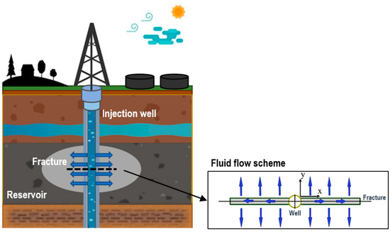
Figure 1.
Fluid-flow scheme: from well to fracture and from fracture to reservoir.
Due to symmetry, one wing of the fracture is considered. The axis will be along the direction of the fracture, and the origin of the coordinates, , is placed on the borehole wall. The axis is directed perpendicular to the plane of the fracture, and counted from the fracture wall (Figure 1).
It is assumed that the reservoir is homogeneous; the fracture width, , is much less than its height, , and the fluid pressure in the fracture depends slightly on the depth. Such a simplified model makes it possible to abandon the third spatial coordinate—depth. Subscripts for variables mean the values related to the fracture or reservoir (porous), and the index 0 means the initial “undisturbed” state.
Let the initial pressure in the reservoir and the fracture be equal to ; for convenience, we will consider that for the pressure in the fracture or reservoir , the deviation from the value (drop), is , instead of writing simply . Note that is a function of the coordinates , and time, , is a function of and .
The system of equations for describing the pressure distribution in the fracture and reservoir (see [8,9,10,11]):
where is the piezoconductivity coefficient, is the porosity is the dynamic fluid viscosity, is the length and is the fracture width.
Equation (1) describes fluid filtration in a fracture, and differs from the classical diffusion-equation (porous medium or heat equation) additional term, which is responsible for the fluid flow between the formation and the hydraulic fracture. Equation (2) has a classical form, and describes fluid filtration in the reservoir perpendicular to the fracture. The equation is solved with respect to the variables and , and in this equation is a parameter. There are boundary conditions:
Condition means that the change in pressure between the reservoir and the fracture occurs continuously. In [9], system (1) and (2) is simplified to one integro-differential equation that describe filtration in a fracture:
Here, we assume that means the system is at rest, i.e., .
By comparing the terms in Equation (3), we obtain critical conditions for the characteristic time, , neglecting the left side of this equation, which determines the elastic capacity of the fluid in the fracture (see [10]). For the problems under consideration, the following estimate holds:
For oilfield problems, it is common to consider values of time (minutes, hours, and days) that always satisfy condition (4). Therefore, instead of (3) we use the simplified equation
Note that Khabibullin and Khisamov’s work [11] also presented the results of modeling the process of non-stationary fluid filtration in a formation penetrated by a well, which was intersected by a vertical hydraulic fracture of finite length throughout the entire thickness of the formation. In this case, Equation (5) was not considered, but system (1) and (2) was directly solved. Results similar to those presented in the next section can be achieved, based on the solutions of this work. Filtration in the reservoir is considered in the case of a finite fracture at constant well-operation modes.
3. Exact Analytical Solutions for Infinite-Length Fracture
In this section we consider a fracture of infinite length and we find the exact analytical solution of Equation (5) for the case of abrupt pressure-changes in the well [12].
3.1. Solutions Corresponding to Piecewise-Constant Laws and a Continuous Change in Well Pressure
In [10] the solution of Equation (5) is given for the case of a sharp change in pressure by a fixed value, , at some point in time Consider solution (5) with the assumption that the fracture-length is infinite .
Suppose that the fluid in the reservoir and fracture is at rest until the moment of time, :
In the case of fluid injection into the reservoir through the fracture, , and in the case of fluid withdrawal, , for definiteness, in what follows, we assume that . Then (see [10]), the solution of Equation (5), which describes the pressure distribution in the hydraulic fracture under the given conditions in which satisfies the condition for , can be written as
Let us pass in (6) to the integration variable, , making the change and introduce a self-similar variable
Solution (6) can be written in terms of a special function
as
Based on this solution, we write the volumetric flow-rate of the fluid in one wing of the fracture per unit of the fracture height as:
From this, we get
It is used here as
—gamma function [13].
Next, consider the case where the pressure at the bottom-hole changes at time points . We assume that, until time , the fluid flow and pressure drops in the fracture and reservoir are equal to zero At the moment of time , the well operation begins, and the pressure in the well, having assumed a value is maintained constant until the moment of time . From the moment of time to the moment of time, the pressure in the well is equal to etc.
Then, the solution describing the pressure change in the fracture is written as
Here,
Further, it is given that, in accordance with to Darcy’s law, the flow-rate per unit of fracture height is as follows [14]:
then
According to [14], Darcy law presents the correlation between the fluid’s viscosity, effective fluid permeability and the fluid pressure-gradient. The law helps determine the flow-rate at any given point in the reservoir. Hence, in accordance with Equations (8) and (9), knowing the change in pressure at the bottom of the well, it is possible to describe the dynamics of pressure in the hydraulic fracture and the fluid flow in the well.
These two equations are generalized to the case when the pressure change in the well is recorded not discretely, but continuously, starting from zero at the time
This is the formula for the pressure change from the initial value in the hydraulic fracture at a distance from the well. Then, the fluid flow-rate per unit-fracture-height is
and after integration by parts, we get
Consider that :
is the formula for changing the fluid flow-rate in the well, in accordance with the known continuous change in well pressure.
3.2. Solutions Corresponding to Piecewis- Constant Laws and a Continuous Change in Well Flow-Rate
Suppose that the fluid in the reservoir and fracture is at rest until the moment of time . At the moment of time the well operation begins in the mode of maintaining a constant fluid-flow:
Nagaeva and Shagapov [10] provided a self-similar solution of Equation (5) for this case:
where the special function is defined as function (Equation (7)):
Substituting into expression (10) the value , we get the law of pressure change in the well
Using the linearity of Equation (5), we generalized the resulting expressions for and to the case when the flow-rate takes constant values in time intervals
is the pressure in the hydraulic fracture in the moment at a distance from the well. The value is assumed to be zero.
For the pressure difference between the values at the bottom hole and in the reservoir , we obtain
A substitution for the expression for from (5) in (11) was made:
Hence, the influence of the formation, fracture and fluid parameters on the law of pressure-drop with a change in flow-rate is noticeable. For practical purposes, one can take the value (see [9,10]).
4. Approximate Analytical Solutions Obtained Using the Method of Sequential Changing of Stationary States for Infinite-Length Fracture
4.1. Application of the Method of Successive Change of Stationary States
According to the method of sequential changing of stationary states [15,16], Equation (2) was solved approximately on the assumption that the reservoir conditionally divided into “disturbed” and “undisturbed” zones at each moment of time. In the undisturbed zone, the pressure was equal to the initial one. The distance, , from the fracture to the boundary of the undisturbed zone was determined by the amount of fluid flowing from the fracture into the reservoir , , —well start-time.
In this case, the steady-state filtration equation is solved in the undisturbed zone, i.e., we assume that the pressure in the reservoir is determined by a linear function with respect to the coordinate :
Equation (13) includes time as a parameter.
In Equation (1), for problems of a practical interest, one can neglect the term on the left side which is responsible for the elasticity of the fluid in the fracture, as we previously did in Section 2. Then, instead of (1), we will consider the equation
Whence, taking into account (13), the equation is:
The result of solving Equation (15) is:
where , —fracture length.
4.2. Solutions Corresponding to Piecewise-Constant Laws and a Continuous Change in Well Pressure in the Case of Infinite-Length Fracture
Consider solution (16) with the assumption that the fracture length is infinite . The comparison of the approximate formulae with field tests carried out in the work showed that the assumption of an infinite fracture-length for most real hydraulic fracturing was quite acceptable to the confirmed practical results.
Suppose the fluid in the fracture and reservoir is at rest until time . Then, from the condition at , we get that, and
Here, is the value of pressure in the well, demonstrated at time . From (17), we receive the following formulae for determining the fluid flow-rate per unit-height of the fracture:
The volume of fluid that was injected into the reservoir or extracted from two fracture wings by the time , after the start of the well operation, was found:
The system of Equations (1) and (2) is linear. Therefore, a linear combination of solutions to this system is again its solution.
Let us generalize Equations (17) and (18) to the case when the pressure takes on piecewise-constant values, changing stepwise at times . We assume that the fluid flow-rates up to time 1 and the pressure-drops in the fracture and reservoir are equal to zero From time to time , the well is operating and the well pressure is kept constant at . From time to time the well pressure is equal to , and so on.
Therefore, the solution obtained by the method of sequential changing of stationary states, which describes the change in the pressure in the fracture, can be written as
The flow-rate of fluid per unit-fracture-height in the well will be equal to
From here, the amount of fluid extracted from two crack arms with a height of was:
4.3. The Law of Pressure Change at a Given Flow-Rate for Infinite-Length Fracture
Consider the well operation in constant-flow-rate mode. The initial state of the formation and fracture is the same as in the previous case, where the fluid flow-rate is zero at time . It is necessary to determine the evolution of the pressure distribution in the fracture, , and the law of pressure change in the well,
From Darcy’s Law:
Let us use solution (16) of Equation (15). at , so we get that
Using Equation (13), it turns out that
And from here, on the well we get ,
Using the linearity of the system of Equations (1) and (2), we generalize the obtained expressions for and to the case where the flow-rate takes constant values in time intervals
The value is assumed to be zero. For the well-pressure difference between the bottom-hole values and the reservoir :
It is interesting to compare these solutions with exact analytic ones (11). The difference between them is only the multipliers and .
4.4. Example of Π—Shaped and Zigzag Flow-Rat-Change
In the case of a Π-shaped change in flow-rate (Figure 2a), which is when the flow-rate at the initial moment of time , is determined by the value , and then returns at the moment of time, , to zero, the estimate from (16) is the formula for determining the pressure change in the hydraulic fracture:
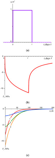
Figure 2.
(a) ∏-shaped change in debit; (b) well-pressure change; (c) pressure evolution in hydraulic fracture.
From here, at , we provide the law of change in well pressure
The parameters of the reservoir and fracture have the following values: kg/m3, , , m/s, m2, , m2, m.
Figure 2b shows the pressure change in the well with a ∏—shaped change in production rate (Figure 2a), up to the value at the initial moment , and returning to the value 0 after 1 day. With a ∏-shaped change in flow-rate, a characteristic tooth is formed on the pressure-change curve. Hydraulic-fracture parameters can be determined by the size of the tooth (see Section 4.5). Figure 2c shows the evolution of pressure in the hydraulic fracture with a ∏—shaped change in well flow-rate, corresponding to Figure 2a. Curve 1 corresponds to the moment of time day, curve 2—1 day, curve 3—1 day and 2 h, curve 4—2 days.
Consider a two-stage change in fluid flow in the well (Figure 3a). Let the fluid-flow-rate per unit of fracture-height be 0 up to time , change by at time and be maintained constant until time then change again to (Figure 3a). It is then convenient to calculate the pressure change in the fracture, based on the formula:
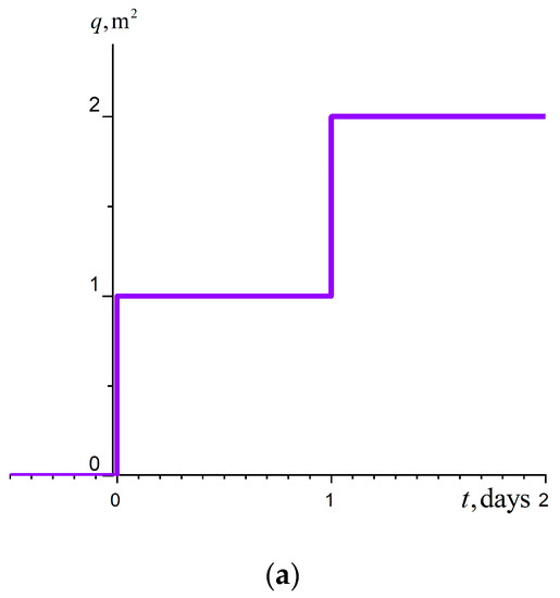
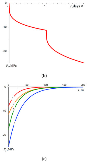
Figure 3.
(a) two-stage change in fluid flow; (b) well-pressure change; (c) pressure evolution in hydraulic fracture.
We find the pressure change in the well, substituting in (23) the value :
Figure 3b shows the change in the well pressure with a stepwise change in flow-rate (Figure 3a), up to the value at the initial moment , and up to the value 2 after 1 day. Figure 3c shows the evolution of pressure in the hydraulic fracture with a stepwise change in pressure in the well, corresponding to Figure 3a. Curve 1 corresponds to the moment of time day, curve 2—1 day, curve 3—1 day and 2 h, curve 4—2 days.
4.5. Determination of Hydraulic Fracture Parameters in Accordance with Well Test-Data
If we have data on pressure changes at the initial time of the well operation and a corresponding change in flow-rate, or there are pressure and flow-rates after a long-term operation of the well in a constant-flow-rate mode and a subsequent sharp change in the operating mode, then using the Formula (17) it is convenient to calculate the parameters of the hydraulic fracture.
Based on Formula (21) the parameters of a fracture with a ∏-shaped flow-rate change were defined. Expressing the value , determined by Formula (5), using the values of the piezoconductivity coefficients from Formulas (1) and (2), we obtain
and from (19), we find the conductivity of the fracture:
5. Approximate Analytical Solutions Obtained Using the Method of Sequential Changing of Stationary States for a Crack of Finite Length
5.1. Solutions Corresponding to Piecewise-Constant Laws and a Continuous Change in Pressure in the Case of Finite-Length Fracture
System (14)–(16) were considered in the previous sections in the case of infinite length fracture. The purpose of this section is to show that in the case of applying the method of sequential changing of stationary states, this assumption does not significantly distort the solution even when considering fractures longer than 50 m.
Consider a fracture of finite length . Let the pressure perturbation in the well be equal to 0 until time (the well did not work), and from time it is kept constant (, ).
The fracture boundary is considered to be impermeable, i.e., .
Considering that from (16) we receive that
From the condition for the pressure in the fracture at the bottom of the well , we find
Then, taking into account (23) and (24), solution (16) takes the form:
From Equation (25), using Darcy’s law, we find the fluid flow-rate per unit fracture height in the well:
Similarly to how it was done in Section 3.1, Formulae (25) and (26) were generalized for the case when the pressure takes on piecewise constant values, changing stepwise at time points . The initial conditions are the same as in Section 2. From time to time , the well pressure is equal , and so on.
Based on solution (25) and using the linearity of system (1) and (2), we find the law of pressure change in the hydraulic fracture:
and fluid flow-rate per unit-fracture-height
5.2. Solutions Corresponding to Piecewies- Constant Laws and a Continuous Change in Flow-Rate in the Case of Finite-Length Fracture
Consider the case where the well is operating in a constant-flow-rate mode. Let the well not function until time point , and then work in constant-flow mode , where the end of fracture is assumed to be closed, as above . Then, from (16), the conditions for determining the constants and are:
Solving this system and substituting the found values and into the general solution (16), we get
From here, under this condition where , the law of change in well pressure is:
Using the linearity of the system Equations (1) and (2), we generalize, as in the previous sections, the obtained expressions for and to the case where the flow-rate takes constant values in time intervals
The value was assumed to be zero. For the pressure difference between the values of the bottom hole and the reservoir , the following was obtained:
If the well flow-rate per unit-fracture-height changes continuously, starting from zero,
Let us compare the pressure-distribution curves in the hydraulic fracture with a ∏-shaped pressure-change in the well, obtained from the formulae for an infinite hydraulic-fracture and for a 50 m long fracture at different points in time.
Let us assume that the well-pressure at time changes by MPa from the initial time and, further, up to time days is maintained constant. At time, the pressure in the well abruptly returns to its original zero-value (Figure 4a). Figure 4b shows the pressure distribution in the fracture for the time points: 1—2 h, 2—1 day, 3—1 day 10 min, 4—1.5 days and 5—3 days for a 50-m-long fracture (solid line) and an infinite crack (dotted line). In Figure 4c, the same comparison is made for a crack 70 m long.
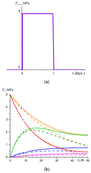
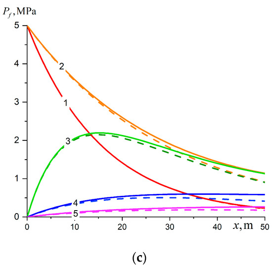
Figure 4.
(a) two-stage pressure change; (b) pressure change in a 50 m long fracture; (c) for a fracture 70 m long. Solid lines—according fracture. 1—2 h, 2—1 day, 3—1 day 10 min, 4—1.5 days and 5—3 days.
A fracture longer than 50 m actually shows the same picture of pressure evolution in a fracture as a fracture of infinite length.
6. Comparison with Practical Data
The authors were provided with field data from one vertical well with hydraulic fracturing from Western Siberia, for research. The curve of flow-rate-change over time is shown in Figure 5a. Some of the results were received using the program registered by the authors [16]. The program uses the approximate formulae obtained by us in Section 4. The parameters have the following values: , m2, . The values of all parameters in the formulae are usually known, except for the fracture conductivity . The value of this parameter can be determined from the ∏-shaped law of flow-rate change and the corresponding change in pressure at the bottom of the well.
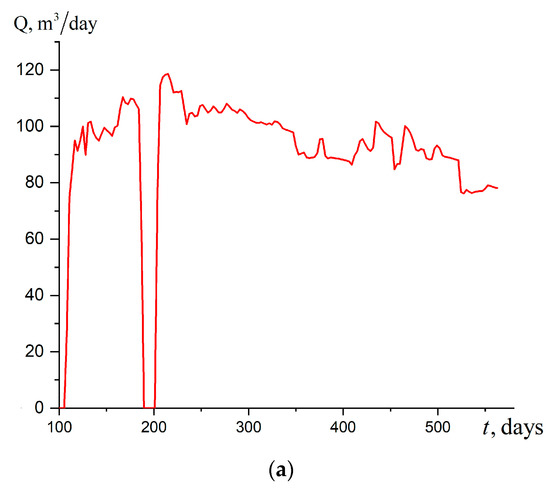
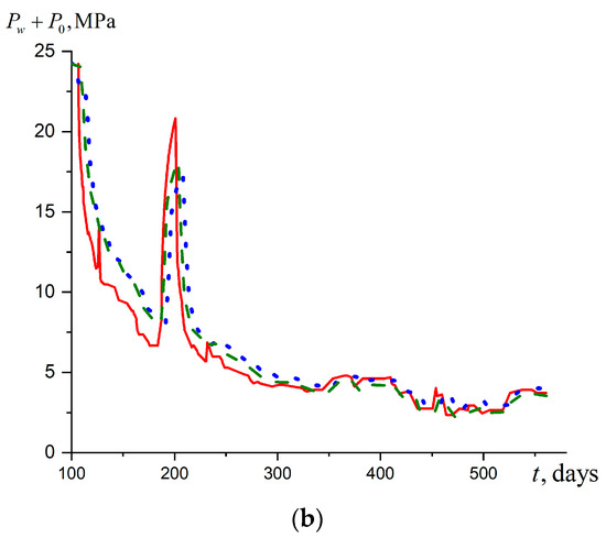
Figure 5.
(a) production rate; (b) the pressure comparison: the initial field pressure (red solid line), analytical formulae (green dashed line) and the approximate method of successive change of stationary-states method (blue dotted line).
Figure 5b shows the pressure comparison: the initial field pressure (red), the results of calculations using the exact analytical Formula (11) (green) and the approximate method of sequential changing of stationary states (20) (blue). At a preliminary stage, in accordance with the first values of the flow-rate jumps and the corresponding values of the real pressure in the well, the fracture conductivity was determined, in accordance with the Formula (20).
It can be seen that the dynamics of the curve change coincide, and the range of values is the same. Thus, the result of comparing the calculations with the actual data allows us to conclude that the constructed mathematical model is capable of reproducing with high accuracy the fluid filtration in a well with a hydraulic fracture during transient-operation modes.
7. Conclusions
As a result of the work, exact and approximate analytical solutions of the system of equations were obtained, which differ little from the exact ones, but are more convenient from a practical point of view. Based on these equations, it is possible to determine the flow-rate or bottom-hole pressure for a given law of change in pressure at the bottom hole or in the well flow-rate, and the evolution of pressure in the hydraulic fracture. The solutions are compared with practical data obtained on real wells. The obtained results can also be used to interpret the results of transient-pressure analysis and the determination of hydraulic-fracture conductivity. In the course of the work, the inverse problem was actually solved to determine the characteristics of the hydraulic fracture. At the same time, if we consider a neighborhood that does not exceed 20–30 m from the well, then, following the results of Section 5, in the case of a fracture length of more than 50 m, it can be considered as an endless fracture.
Let us pay attention to the fact that in order to determine the parameters of a hydraulic fracture, the well must be at rest for a long time or operate in a constant-flow-rate mode for a long time. This is due to the fact that in solutions (19) and (20), each new term was added to the previous ones. The action of the previous terms does not stop, but only slowly weakens. At the same time, it would be interesting to solve the problem of determining the parameters of the reservoir based on arbitrary sections of the “rate—pressure” curves.
Author Contributions
Investigation, R.A.B., N.O.F. and A.A.S.; Supervision, V.S.S. All authors have read and agreed to the published version of the manuscript.
Funding
This research was funded by the Russian Science Foundation: grant No. 21-11-00207, https://rscf.ru/project/21-11-00207/.
Conflicts of Interest
The authors declare no conflict of interest.
References
- Economides, M.; Oligney, R.; Valko, P. Unified Fracture Design Bridging the Gap between Theory and Practice; Orsa Pressin: Alvin, TX, USA, 2002; p. 237. [Google Scholar]
- Zheltov, Y.P.; Khristianovich, S.A. Hydraulic Fracturing of an Oil Reservoir. Izv. Akad. Nauk SSSR Otdel. Tekhn. Nauk 1955, 5, 3–41. (In Russian) [Google Scholar]
- Geertsma, J.; De Klerk, F. A Rapid Method of Predicting Width and Extent of Hydraulically Induced Fractures. J. Pet. Technol. 1969, 21, 1571–1581. [Google Scholar] [CrossRef]
- Nordgren, R.P. Propagation of a Vertical Hydraulic Fracture. SPE J. 1972, 12, 306–314. [Google Scholar] [CrossRef]
- Perkins, T.; Kern, L. Widths of Hydraulic Fractures. J. Pet. Technol. 1961, 222, 937–949. [Google Scholar] [CrossRef]
- Gringarten, A.C.; Ramey, H.J.J. Unsteady-State Pressure Distributions Created by a Well with a Single Horizontal Fracture, Partial Penetration, or Restricted Entry. SPE J. 1974, 14, 413–426. [Google Scholar] [CrossRef]
- Cinco-Ley, H.; Samaniego, F.; Dominguez, N. Transient Pressure Behavior for a Well with a Finite-Conductivity Vertical Fracture. SPE J. 1978, 18, 253–264. [Google Scholar] [CrossRef]
- Khabibullin, I.L.; Khisamov, A.A. Unsteady Flow through a Porous Stratum with Hydraulic Fracture. Fluid Dyn. 2019, 54, 594–602. [Google Scholar] [CrossRef]
- Shagapov, V.S.; Nagaeva, Z.M. On the theory of seepage waves of pressure in a fracture in a porous permeable medium. J. Appl. Mech. Tech. Phys. 2017, 58, 862–870. [Google Scholar] [CrossRef]
- Nagaeva, Z.; Shagapov, V. Elastic Seepage in a Fracture Located in an Oil or Gas Reservoir. J. Appl. Math. Mech. 2017, 81, 214–222. [Google Scholar] [CrossRef]
- Khabibullin, I.L.; Khisamov, A.A. Modeling of unsteady fluid filtration in a reservoir with a hydraulic fracture. J. Appl. Mech. Tech. Phys. 2022, 63, 652–660. [Google Scholar] [CrossRef]
- Shagapov, V.S.; Bashmakov, R.A.; Fokeeva, N.O. Fluid filtration in reservoirs subjected to hydraulic fracturing during transient well operation. J. Appl. Mech. Tech. Phys. 2022, 63, 474–483. [Google Scholar] [CrossRef]
- Whittaker, E.T.; Watson, G.N. A Course of Modern Analysis; Merchant Books: Tapa del libro, Blanda, 2008. [Google Scholar]
- Animasaun, I.L.; Shah, N.A.; Wakif, A.; Mahanthesh, B.; Sivaraj, R.; Koriko, O.K. Ratio of Momentum Diffusivity to Thermal Diffusivity: Introduction, Meta-Analysis, and Scrutinization; Chapman and Hall/CRC: New York, NY, USA, 2022; ISBN1 978-1032108520. ISBN2 1032108525. ISBN3 9781003217374. (In Russian) [Google Scholar]
- Shagapov, V.S.; Nagaeva, Z.M. Approximate Solution of the Problem on Elastic-Liquid Filtration in a Fracture Formed in an Oil Stratum. J. Eng. Phys. Thermophy 2020, 93, 201–209. [Google Scholar] [CrossRef]
- Shagapov, V.S.; Bashmakov, R.A.; Shammatova, A.A. Determination of pressure changes at the bottom of an oil well during work placement. Certificate of registration of the computer program 2022667756, 26 September 2022. eLIBRARY ID: 49775186 EDN: LKZZPK.


Disclaimer/Publisher’s Note: The statements, opinions and data contained in all publications are solely those of the individual author(s) and contributor(s) and not of MDPI and/or the editor(s). MDPI and/or the editor(s) disclaim responsibility for any injury to people or property resulting from any ideas, methods, instructions or products referred to in the content. |
© 2022 by the authors. Licensee MDPI, Basel, Switzerland. This article is an open access article distributed under the terms and conditions of the Creative Commons Attribution (CC BY) license (https://creativecommons.org/licenses/by/4.0/).