An Improved Mixture Model of Gaussian Processes and Its Classification Expectation–Maximization Algorithm

Abstract

The mixture of experts (ME) model is effective for multimodal data in statistics and machine learning. To treat non-stationary probabilistic regression, the mixture of Gaussian processes (MGP) model has been proposed, but it may not perform well in some cases due to the limited ability of each Gaussian process (GP) expert. Although the mixture of Gaussian processes (MGP) and warped Gaussian process (WGP) models are dominant and effective for non-stationary probabilistic regression, they may not be able to handle general non-stationary probabilistic regression in practice. In this paper, we first propose the mixture of warped Gaussian processes (MWGP) model as well as its classification expectation–maximization (CEM) algorithm to address this problem. To overcome the local optimum of the CEM algorithm, we then propose the split and merge CEM (SMC EM) algorithm for MWGP. Experiments were done on synthetic and real-world datasets, which show that our proposed MWGP is more effective than the models used for comparison, and the SMCEM algorithm can solve the local optimum for MWGP.

1. Introduction

The mixture of experts (ME) model is effective for multimodal data in statistics and machine learning [1]. In ME, the input space is softly divided into multiple regions by an input-dependent gating function, and each region is specified by an expert. Due to the diversity of experts, such as Gaussian distribution [2] and the support vector machine (SVM) [3], there are a variety of models based on the ME framework.

In the 2000s, Tresp constructed the mixture of Gaussian processes (MGP) model, a special ME where each expert is a stationary Gaussian process (GP) probabilistic regression model, by mixing GPs along the input space to treat non-stationary probabilistic regression [4,5,6,7,8]. Popular gating functions of the MGP include logistic distribution and Gaussian distribution. For learning MGP, the main algorithms are Markov Chain Monte Carlo (MCMC), variational Bayesian (VB), and expectation–maximization (EM). The MGP cannot work correctly on non-stationary probabilistic regression in some situations since the ability of each GP expert is limited.

In this paper, we propose the mixture of warped Gaussian processes (MWGP) model, which has more flexible and attractive properties than MGP to handle non-stationary probabilistic regression, by modeling each component of an MGP with a warped Gaussian process (WGP); these WGPs are combined in the input space by the Gaussian distribution. The WGP is capable of modeling non-stationary probabilistic regression by learning a nonlinear distortion (also called warping) of the GP outputs. The MWGP can be viewed as a generalization of the MGP and WGP frameworks, and it allows for dealing with non-stationary data in each multimodal mode. In MWGP, the mixture parameter, warping function parameter, covariance function parameter, and indicator variable (regarded as the latent variable) are considered simultaneously. To handle this, we designed the classification expectation–maximization (CEM) algorithm for the training of MWGP. However, the CEM algorithm may easily converge to a local optimum for MWGP in some cases. We propose the split and merge CEM (SMCEM) algorithm of MWGP based on the SMCEM algorithm of the MGP and the CEM algorithm of MWGP to solve this problem. Experiments were conducted on synthetic and real-world datasets, and the results demonstrate the feasibility and superior accuracy of our proposed MWGP model trained using the CEM algorithm compared to other comparative models for probabilistic regression. Moreover, the SMCEM algorithm of MWGP can overcome local optima in some datasets at a negligible time cost.

The remainder of this paper is organized as follows. In Section 2, we present related works of GP, MGP, and WGP models. We describe GP, WGP, and our proposed MWGP in Section 3. In Section 4, we present our proposed SMCEM algorithm of MWGP, the CEM algorithm of MWGP, and the partial CEM algorithm of MWGP. The experimental results are presented in Section 5, and the conclusions are drawn in Section 6.

2. Related Works

Related works of the GP. The GP is a versatile tool for probabilistic regression and it has been successfully applied to practical fields such as time series prediction [9] and signal processing [10]. The non-stationary probabilistic regression problem exists widely, but it cannot be modeled effectively by the conventional GP model [11,12]. To solve this, the non-stationary GP model was proposed by introducing a robust and flexible covariance structure [13,14,15,16]. However, a single GP cannot handle the non-stationary probabilistic regression well due to its inherent simplicity.

Related works of the MGP model. The structure of the MGP is shown in Figure 1. As seen in this figure, the MGP is a more effective non-stationary model than the GP. However, the parameter estimation of the MGP is a challenge due to the unknown indicator variable (regarded as the latent variable) and the highly correlated sample [17,18,19,20]. The Markov Chain Monte Carlo (MCMC) method employing Gibbs sampling and hybrid Monte Carlo approximates the intractable integration and summation by the simulated sample of the indicator variable and parameter [6,7,21,22,23], and it is commonly used in a system of partial differential equations [24,25]. The MCMC generally obtains precise results, but it takes a long time to generate the simulated sample. To improve the efficiency, the variational Bayesian (VB) inference and the expectation–maximization (EM) algorithm were proposed. Ross and Dy constructed the VB inference on the basis of the mean-field approximation, where the indicator variable and the stochastic parameter are forced to be independent of the probability distribution [26]. Yuan and Neubauer established a variational EM algorithm by a similar mean-field method as the VB inference [8]. Then, the leave-one-out cross-validation (LOOCV) EM algorithm was proposed based on the LOOCV approximation method, where the probability density of the GP is approximated by the production of LOOCV probability densities [27]. To improve the accuracy, Chen et al. constructed the CEM algorithm by replacing the expectation step (E step) of the conventional EM algorithm with a classification–expectation step (CE step) [28,29]. For the CEM algorithm, samples are classified into components by the maximum a posteriori (MAP) principle of indicator variables in the CE step and the parameters of components are learned independently in the maximization step (M step). Then, the MCMC EM algorithm was designed by approximating the Q-function of the EM algorithm with the Gibbs sampling; this algorithm is generally accurate but slow [30,31,32]. The SMCEM algorithm was constructed by combining the split and merge EM algorithm and the CEM algorithm to address the local optimum of the CEM algorithm for MGP [33,34,35,36]. Regarding the model selection problem, i.e., selecting the number of components, the Dirichlet process as the gating function was developed [6,17,21,22]; moreover, Zhao and Ma proposed a synchronous balancing criterion [37]. Regarding the robustness problem, the robust MGP with the Laplace noise and the robust MGP with the student-t noise were proposed to overcome this difficulty [38].

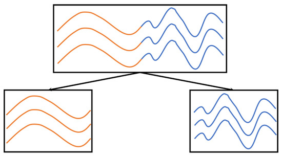
Figure 1. The diagram structure of the MGP model: the low-layer consists of two GPs and the high-layer structure consists of an MGP. The curves are divided into two curve segments along the input space marked in different colors, and curve segments of one color corresponding to a GP.

Related works of the WGP model. The WGP trained by the maximum likelihood estimation (MLE) method can handle non-stationary probabilistic regression effectively by transforming the GP output in a latent space to the real output in the observation space with a learnable nonlinear monotonic function [39], as seen in Figure 2. From this figure, it is clear that the WGP is much better than the GP, and the performance of the GP degenerates dramatically. In WGP, such a preprocessing transformation can be considered as an integral part of non-stationary probabilistic modeling. The improved WGP models involve a large number of parameters and hyperparameters, which limits the applicability of the WGP. The Hamiltonian MCMC method [40] and the VB inference [41] were proposed to improve the training of the WGP in some situations. To make the WGP structure flexible, Rios et al. constructed the WGP with a deep compositional architecture warping function [42], and the multi-task WGP was proposed [43]. For the optimization of the WGP, a spatial branching strategy was designed [44]. The WGP (being a useful generalization of the GP) has also been widely used in practical applications [45,46,47,48].

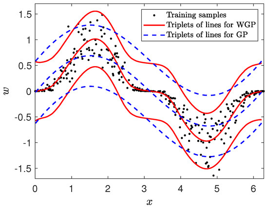
Figure 2. An example of a non-stationary data regression task. The one-dimensional data are generated by adding Gaussian noise to a sine function. The dataset contains 300 training samples and 600 test samples. These samples are then warped by the function $w=y^3.$ The mean and two standard deviation (SD) bounds are represented by triplets of lines.

3. Model Construction

In this section, we first introduce the GP and WGP models and then describe our proposed MWGP model.

3.1. The GP

The GP is a non-parametric statistical model, which is described briefly as follows. For a dataset ${\{{\mathbf{x}}_n\in {\mathbb{R}}^E,y_n\in \mathbb{R}\}}_{n=1}^N,$ the standard Gaussian process (GP) model for probabilistic regression is defined by

$$y_n=f\left({\mathbf{x}}_n\right)+{\epsilon }_n\mathrm{and}{\epsilon }_n\sim \mathrm{N}\left(0,{\sigma }^2\right),$$

(1)

where $f(•)$, $y_n$, ${\mathbf{x}}_n$, ${\epsilon }_n$, and $\sigma$ are the random latent function described, the n-th output, the n-th $E\times 1$ input, the n-th Gaussian noise, and the SD of the Gaussian noise, respectively. The random latent function $f(•)$ on ${\left\{{\mathbf{x}}_n\right\}}_{n=1}^N$ is subject to a Gaussian distribution

$$p\left(\mathbf{f}\right|\mathbf{X})=N(\mathsf{\mu },\mathbf{K}),$$

where $\mathbf{X}=[{\mathbf{x}}_1,{\mathbf{x}}_2,\cdots ,{\mathbf{x}}_N]$ is the $E\times N$ input matrix, $\mathbf{f}={\left[f_n\right]}_{N\times 1}$ is the latent vector, $f_n=f\left({\mathbf{x}}_n\right)$, $\mathsf{\mu }={\left[{\mu }_n\right]}_{N\times 1}$ is the mean vector, ${\mu }_n=\mu \left({\mathbf{x}}_n\right)$ is the mean function, $\mathbf{K}={\left[K_{n\tilde{n}}\right]}_{N\times N}$ is the covariance matrix, and $K_{n\tilde{n}}=K({\mathbf{x}}_n,{\mathbf{x}}_{\tilde{n}};\mathsf{\gamma })$ is the covariance function (In this paper, we use the squared exponential covariance function

$$K({\mathbf{x}}_n,{\mathbf{x}}_{\tilde{n}};\mathsf{\gamma })={\left({\gamma }^{\left(1\right)}\right)}^2\exp \left[-{({\mathbf{x}}_n-{\mathbf{x}}_{\tilde{n}})}^{\mathrm{T}}\mathsf{\Lambda }({\mathbf{x}}_n-{\mathbf{x}}_{\tilde{n}})/2\right],$$

where $\mathsf{\Lambda }=diag\left(1/{\left({\gamma }^{\left(2\right)}\right)}^2,1/{\left({\gamma }^{\left(3\right)}\right)}^2,\cdots ,1/{\left({\gamma }^{(E+1)}\right)}^2\right)$ is the $E\times E$ diagonal matrix) parameterized by $\mathsf{\gamma }=[{\gamma }^{\left(1\right)},{\gamma }^{\left(2\right)},\cdots ,{\gamma }^{(E+1)}]$

The likelihood function of the GP is obtained by integrating $p\left(\mathbf{y}\right|\mathbf{f}\left)p\right(\mathbf{f}\left|\mathbf{X}\right)$ with respect to $\mathbf{f}$, given by

$$p\left(\mathbf{y}\right|\mathbf{X})=N(\mathsf{\mu },\mathbf{K}+{\sigma }^2{\mathbf{I}}_{\mathit{N}}),$$

(2)

where $p\left(\mathbf{y}\right|\mathbf{f})$ is the independent identically distributed Gaussian distribution obtained by Equation (1), $\mathbf{y}={\left[y_n\right]}_{N\times 1}$ is the output vector, and ${\mathbf{I}}_N$ is the $N\times N$ unit matrix.

3.2. The WGP Model

In the non-stationary probabilistic regression problem, the WGP model describes the real output in the observation space as a parametric nonlinear transformation of the GP. For the dataset $\mathcal{D}={\{{\mathbf{x}}_n\in {\mathbb{R}}^E,w_n\in \mathbb{R}\}}_{n=1}^N,$ the WGP is constructed by introducing a latent variable set ${\{y_n\in \mathbb{R}\}}_{n=1}^N$, where $w_n$ and ${\mathbf{x}}_n$ are the n-th output in the observation space and the n-th $E\times 1$ input, respectively. The latent vector $\mathbf{y}={\left[y_n\right]}_{N\times 1}$ is subject to a GP with a zero-mean function (i.e., $\mu \left({\mathbf{x}}_n\right)=0$), defined by Equation (2)

$$p\left(\mathbf{y}\right|\mathbf{X})=N({\mathbf{0}}_{N\times 1},\mathbf{K}+{\sigma }^2{\mathbf{I}}_{\mathit{N}}).$$

The latent variable $y_n$ is transformed to $w_n$ by a monotonic warping function (In this paper, we assume the warping function to be a feedforward neural network $g(w_n;\mathsf{\Omega })=w_n+{\sum }_{j=1}^J{a}_{j}tanh\left(h_j(w_n+l_j)\right),$ where $a_j$ and $h_j$ are non-negative for any j to ensure monotonicity, J is the number of neurons, and $\mathsf{\Omega }={[a_1,a_2,\cdots ,a_J,h_1,h_2,\cdots ,h_J,l_1,l_2,\cdots ,l_J]}^{\mathrm{T}}$). $g(•;\mathsf{\Omega })$

$$y_n=g(w_n;\mathsf{\Omega }),$$

where $g(w_n;\mathsf{\Omega })$ maps $w_n$ to the entire real line, and $\mathsf{\Omega }$ is the parameter vector composed of J neurons. As stated above, the established WGP is fully incorporated into the probabilistic framework of the GP.

For convenience, the WGP is denoted as

$$\mathbf{w}\sim \mathrm{WGP}(\mathbf{X};\mathsf{\theta },\mathsf{\Omega }),$$

(3)

where $\mathbf{w}={\left[w_n\right]}_{N\times 1}$ is the output vector and $\mathsf{\theta }=\{\sigma ,{\gamma }^{\left(1\right)},{\gamma }^{\left(2\right)},\cdots ,{\gamma }^{(E+1)}\}$. For WGP, the information flow direction is ${\mathbf{x}}_n\to y_n\to w_n$, and the relationships between the main variables are shown in Figure 3. From this figure, outputs ${\{w_n\in \mathbb{R}\}}_{n=1}^N$ are conditionally independent when the strongly correlated ${\left\{f_n\right\}}_{n=1}^N$ are given. The parameters $\mathsf{\theta }$ and $\mathsf{\Omega }$ are learned jointly using a conjugate gradient method for WGP.

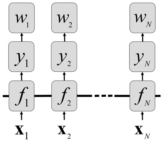
Figure 3. A diagram showing the relations among the main variables in the WGP model.

3.3. The MWGP Model

To process multimodal data while modeling the non-stationary nature of each mode, we describe our proposed MWGP model mathematically next, where C-different WGP components are mixed in the input region. The structure of MWGP is similar to that of the MGP, as illustrated in Figure 1. Compared to the MGP, the two-layer structure of MWGP can address non-stationary probabilistic regression in different ways.

A subscript c is inserted in the preceding notation for the number of components. The n-th sample $({\mathbf{x}}_n,w_n)$ is allocated to the c-th WGP component by an indicator variable $z_{nc}$ (regarded as a latent variable), where $c=1,2,\cdots ,C$. If $({\mathbf{x}}_n,w_n)$ is in the c-th component, then $z_{nc}$ = 1; otherwise, $z_{nc}$ = 0. The distribution of the indicator variable vector ${\mathbf{z}}_n={[z_{n1},z_{n2},\cdots ,z_{nC}]}^{\mathrm{T}}$ is given by

$$P({\mathbf{z}}_n={\mathbf{e}}_c)={\eta }_c,$$

(4)

where ${\mathbf{e}}_c$ is the c-th column of the $C\times C$ unit matrix ${\mathbf{I}}_{\mathit{C}}$ and ${\sum }_{c=1}^C{\eta }_c=1.$

The distribution of the input vector ${\mathbf{x}}_n$ is given by

$$p\left({\mathbf{x}}_n\right|{\mathbf{z}}_n={\mathbf{e}}_c)=\mathrm{N}({\mathsf{\alpha }}_c,{\mathsf{\Sigma }}_c),$$

(5)

where ${\mathsf{\alpha }}_c$ and ${\mathsf{\Sigma }}_c$ are the $E\times 1$ mean vector and the $E\times E$ covariance matrix of the Gaussian distribution, respectively. Equation (5) is commonly used in most generative mixture models.

After the distributions of Equations (4) and (5) are given, the distribution of the output vector ${\mathbf{w}}_c$ is given based on Equation (3) by

$${\mathbf{w}}_c\sim \mathrm{WGP}({\mathbf{X}}_c;{\mathsf{\theta }}_c,{\mathsf{\Omega }}_c),$$

(6)

where ${\mathbf{X}}_c$ is the $E\times N_c$ input matrix composed of $\left\{{\mathbf{x}}_n\right|{\mathbf{z}}_n={\mathbf{e}}_c;n=1,2,\cdots ,N\}$ in which $N_c={\sum }_{n=1}^N{z}_{nc}$ is the sample number, ${\mathbf{w}}_c$ is the $N_c\times 1$ output vector composed of $\left\{w_n\right|{\mathbf{z}}_n={\mathbf{e}}_c;n=1,2,\cdots ,N\}$, ${\mathsf{\Omega }}_c$ parameterizes the warping function of the c-th component, and ${\mathsf{\theta }}_c=\{{\sigma }_c,{\gamma }_c^{\left(1\right)},{\gamma }_c^{\left(2\right)},\cdots ,{\gamma }_c^{(E+1)}\}$. For MWGP, C WGP components are independent, and each component is defined by Equation (6). MWGP is generally more flexible than the MGP and WGP; its information flow direction is ${\mathbf{z}}_n\to {\mathbf{x}}_n\to y_n\to w_n$, as shown in Figure 4. If $C=1,$ then the MWGP degenerates to WGP; if $g(w_n;{\mathsf{\Omega }}_c)=w_n$, then the MWGP degenerates to MGP.

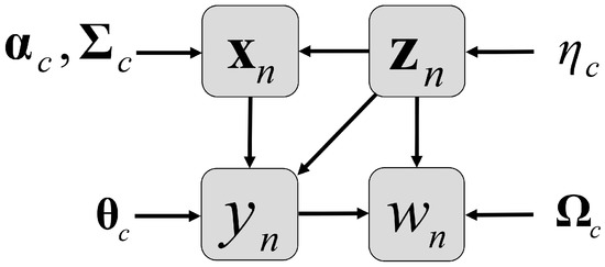
Figure 4. The probabilistic graphical model of the MWGP model: the elements inside the boxes are main variables and the others are parameters.

With the above analysis, the mixture structure, the covariance function, and the warping function are incorporated simultaneously in the same probabilistic model framework. The computational cost of MWGP is similar to MGP since the time complexity of the inverse covariance matrix operation in MWGP is the same as that in MGP, i.e., $O(N^3/C^2)$. For MWGP, there is an overfitting problem when too many extra parameters are added.

4. Algorithm Design

To handle the large time complexity of calculating the Q-function in the conventional EM algorithm of MWGP, we designed the CEM and partial CEM algorithms. In the CEM algorithm of MWGP, a local optimum is generally generated when there is a large separation between two parts of the MWGP component in practice. This separation is created by having many components of MWGP in one region and few in another. To escape from this separation, simultaneous split and merge operations were performed repeatedly by merging two similar components in a region with many components and splitting one component in another region with few components. As the CEM algorithm of MWGP can sometimes get trapped in a local optimum, we developed the SMCEM algorithm of MWGP to address this issue. The CEM algorithm of MWGP and the partial CEM algorithm of MWGP are sub-algorithms of the SMCEM algorithm for MWGP.

4.1. Procedures of the Proposed Algorithms

Denote the $C\times N$ indicator variable matrix $\mathbf{Z}=[{\mathbf{z}}_1,{\mathbf{z}}_2,\cdots ,{\mathbf{z}}_N]$ and the whole parameter set $\mathsf{\Phi }={\left\{{\mathsf{\Phi }}_c\right\}}_{c=1}^C$, where ${\mathsf{\Phi }}_c=\{{\eta }_c,{\mathsf{\alpha }}_c,{\mathsf{\Sigma }}_c,{\mathsf{\theta }}_c,{\mathsf{\Omega }}_c\}$. For MWGP, procedures of the SMCEM algorithm, the CEM algorithm, and the partial CEM algorithm are presented in Algorithms 1–3.

Algorithm 1 The SMCEM algorithm for MWGP

Input: $\mathcal{D},C,J.$ Output: ${\mathsf{\Phi }}_{best},{\mathrm{L}}_{best}.$ 1: Initialization: Initialize the indicator variable matrix ${\mathbf{Z}}^{\left(0\right)}$ by the k-means clustering on the input set ${\left\{{\mathbf{x}}_n\right\}}_{n=1}^N$, and obtain the indicator variable matrix ${\mathbf{Z}}^{\left(1\right)}$ and the parameter set ${\mathsf{\Phi }}^{\left(0\right)}$ by performing the CEM algorithm described in Algorithm 2. Set the number of current iterations as $r=1$, and ${\mathrm{L}}_{best}=-\infty$. 2: The merge operation: The component numbers of the merge operation u and s are obtained by the merge criterion described in Appendix C, where $u,s\in \{1,2,\cdots ,C\}$ and $u\ne s$. The new component after merging the old u-th component and the old s-th component is called the u-th component. 3: The split operation: The component number of the split operation t is obtained by the split criterion described in Appendix C, where $t\in \{1,2,\cdots ,C\}$. New components after splitting the old t-th component are called the s-th and t-th components. 4: For $n\in \left\{n\right|{\mathbf{z}}_n^{(3r-2)}={\mathbf{e}}_s\}$, set ${\mathbf{z}}_n^{(3r-1)}={\mathbf{e}}_u;$$\left\{{\mathbf{x}}_n\right|{\mathbf{z}}_n^{(3r-2)}={\mathbf{e}}_t;n=1,2,\cdots ,N\}$ is clustered into two clusters by the k-means clustering, and set ${\mathbf{z}}_n^{(3r-1)}={\mathbf{e}}_s$ for samples of the first cluster; otherwise, set ${\mathbf{z}}_n^{(3r-1)}={\mathbf{z}}_n^{(3r-2)}$. 5: Obtain ${\mathbf{Z}}^{\left(3r\right)}$ by performing the partial CEM algorithm described in Algorithm 3. 6: Obtain ${\mathsf{\Phi }}^{\left(3r\right)}$ and ${\mathbf{Z}}^{(3r+1)}$ by performing the the CEM algorithm described in Algorithm 2. 7: Convergence criterion: If the value of the approximated Q-function $\mathrm{L}({\mathsf{\Phi }}^{\left(3r\right)},{\mathbf{Z}}^{(3r+1)})>{\mathrm{L}}_{best}$, then set ${\mathrm{L}}_{best}=\mathrm{L}({\mathsf{\Phi }}^{\left(3r\right)},{\mathbf{Z}}^{(3r+1)})$, ${\mathsf{\Phi }}_{best}={\mathsf{\Phi }}^{\left(3r\right)}$, $r=r+1$ and return to the second step; otherwise, stop.

Algorithm 2 The CEM algorithm for MWGP

Input: $\mathcal{D},C,J.$ Output: ${\mathsf{\Phi }}^{\left(r^{\prime }\right)},{\mathbf{Z}}^{\left(r^{\prime }\right)}.$ 1: Initialization: Set the initialized indicator variable matrix ${\mathbf{Z}}^{\left(0\right)}={\mathbf{Z}}^{\left(3r\right)}$ (or ${\mathbf{Z}}^{\left(0\right)}$) and $r^{\prime }$ = 1. 2: M step: Update ${\mathsf{\Phi }}^{\left(r^{\prime }\right)}$ by maximizing $\mathrm{L}(\mathsf{\Phi },{\mathbf{Z}}^{(r^{\prime }-1)})$ described in Appendix A.2. 3: CE step: Update ${\mathbf{Z}}^{\left(r^{\prime }\right)}$ by the approximated MAP principle described in Appendix A.1. 4: Convergence criterion: If $r^{\prime }>9$ and $$\begin{array}{cc}\hfill & \left({\sum }_{i=r^{\prime }-4}^{r^{\prime }}\mathrm{L}({\mathsf{\Phi }}^{\left(i\right)},{\mathbf{Z}}^{\left(i\right)})-{\sum }_{i=r^{\prime }-9}^{r^{\prime }-5}\mathrm{L}({\mathsf{\Phi }}^{\left(i\right)},{\mathbf{Z}}^{\left(i\right)})\right)/\left|{\sum }_{i=r^{\prime }-9}^{r^{\prime }-5}\mathrm{L}({\mathsf{\Phi }}^{\left(i\right)},{\mathbf{Z}}^{\left(i\right)})\right|<ϵ,\hfill \end{array}$$ or $r^{\prime }\ge r_{max}$, stop; otherwise, $r^{\prime }=r^{\prime }+1$ and return to the second step.

Algorithm 3 The partial CEM algorithm for MWGP.

Input: $\mathcal{D},u,s,t,J.$ Output: ${\mathbf{Z}}^{\left(r^{″}\right)}.$ 1: Initialization: Set the initialized indicator variable matrix ${\mathbf{Z}}^{\left(0\right)}={\mathbf{Z}}^{(3r-1)}$ and $r^{″}$ = 1. 2: Partial M step: Update ${\mathsf{\Phi }}_{c=u,s,t}^{\left(r^{″}\right)}$ by partially maximizing $\mathrm{L}(\mathsf{\Phi },{\mathbf{Z}}^{(r^{″}-1)})$, as described in Appendix B.1. 3: Partial CE step: Obtain ${\mathbf{z}}_n^{\left(r^{″}\right)}$ for $n\in \left\{n\right|{\mathbf{z}}_n^{(r^{″}-1)}={\mathbf{e}}_{c=u,s,t}\}$ by the approximated MAP principle described in Appendix B.2; otherwise, set ${\mathbf{z}}_n^{\left(r^{″}\right)}={\mathbf{z}}_n^{(r^{″}-1)}$. 4: Convergence criterion: If $r^{″}>$9 and $$\begin{array}{cc}\hfill & \left({\sum }_{i=r^{″}-4}^{r^{″}}\mathrm{L}({\mathsf{\Phi }}^{\left(i\right)},{\mathbf{Z}}^{\left(i\right)})-{\sum }_{i=r^{″}-9}^{r^{″}-5}\mathrm{L}({\mathsf{\Phi }}^{\left(i\right)},{\mathbf{Z}}^{\left(i\right)})\right)/\left|{\sum }_{i=r^{″}-9}^{r^{″}-5}\mathrm{L}({\mathsf{\Phi }}^{\left(i\right)},{\mathbf{Z}}^{\left(i\right)})\right|<ϵ,\hfill \end{array}$$ or $r^{″}\ge r_{max}$, stop; otherwise, $r^{″}=r^{″}+1$ and return to the second step.

The k-means clustering method is adopted in the first step of Algorithm 1 since it is possible for some samples to belong to the same component if they are close in distance. In the second and third steps of Algorithm 1, the split candidate set $\left\{t\right\}$ and the merge candidate set $\{u,s\}$ are sorted by split and merge criteria, respectively. By renumbering the merge and split candidate sets, we obtain the candidate set $\{u,s,t\}$. In the fifth step of Algorithm 1, we perform the partial CEM algorithm to retrain the parameters of new components and ensure that all other components are not affected by this retraining. The CEM algorithm is performed as a full training procedure for all components in the sixth step of Algorithm 1. In the seventh step of Algorithm 1, it is obvious that the accepted split or merge operation attempts to increase the value of the approximated Q-function in each iteration. We set hyperparameters $C$, J, and D according to the best RMSE (the root mean square error (RMSE) is used to characterize the accuracy of the model, which is defined mathematically by $\sqrt{{\sum }_{n=1}^N{(y_n-{\widehat{y}}_n)}^2/N}$, where ${\widehat{y}}_n$ is the estimation of $y_n$). In Algorithm 1, components of MWGP with poor aggregation are divided in the split operation, and those with high similarity are combined in the merge operation. Simultaneous split and merge operations can perform a global search by crossing over low-likelihood positions.

In the second and third steps of Algorithm 2, $\mathsf{\Phi }$ and $\mathbf{Z}$ are updated alternately. Samples are classified into C components to overcome the time complexity of the conventional EM algorithm in the third step of Algorithm 2. In the fourth step of Algorithm 2, we apply a relatively long-term convergence criterion.

$$\begin{array}{c}\hfill \left({\sum }_{i=r^{\prime }-4}^{r^{\prime }}\mathrm{L}({\mathsf{\Phi }}^{\left(i\right)},{\mathbf{Z}}^{\left(i\right)})-{\sum }_{i=r^{\prime }-9}^{r^{\prime }-5}\mathrm{L}({\mathsf{\Phi }}^{\left(i\right)},{\mathbf{Z}}^{\left(i\right)})\right)/\left|{\sum }_{i=r^{\prime }-9}^{r^{\prime }-5}\mathrm{L}({\mathsf{\Phi }}^{\left(i\right)},{\mathbf{Z}}^{\left(i\right)})\right|<ϵ\end{array}$$

since $\mathrm{L}({\mathsf{\Phi }}^{\left(r^{\prime }\right)},{\mathbf{Z}}^{\left(r^{\prime }\right)})$ may fluctuate during iterations, we present the largest number of iterations, i.e., $r_{max}$ = 30 and $ϵ$ = 0.002. Regarding the annealing mechanism, Algorithm 2 can be viewed as a deterministic annealing EM algorithm with the annealing parameter tending to positive infinity, while the conventional EM algorithm can be viewed as a deterministic annealing EM algorithm with the annealing parameter being one. Theoretically, Algorithm 2 is more likely to fall into a local optimum than the conventional EM algorithm. The details of the CEM algorithm are described in Appendix A.

Algorithm 3 was performed on new components generated by the simultaneous split and merge operations. In the second and third steps of Algorithm 3, ${\mathsf{\Phi }}_{c=u,s,t}^{\left(r^{″}\right)}$ and ${\mathbf{z}}_n^{\left(r^{″}\right)}$ are updated alternately, where $n\in \left\{n\right|{\mathbf{z}}_n^{(r^{″}-1)}={\mathbf{e}}_{c=u,s,t}\}$. In the third step of Algorithm 3, ${\mathbf{z}}_n^{\left(r^{″}\right)}$ for $n\in \left\{n\right|{\mathbf{z}}_n^{(r^{″}-1)}={\mathbf{e}}_{c=u,s,t}\}$ is obtained by using the initialized ${\mathbf{Z}}^{(3r-1)}$, while ${\mathbf{z}}_n^{\left(r^{″}\right)}={\mathbf{z}}_n^{(r^{″}-1)}$ is set for the other components. The details of the partial CEM algorithm are described in Appendix B.

4.2. Prediction Strategy

For MWGP, the time complexity of the conventional prediction method is generally high. We adopted the classification approximation method for MWGP to improve the predictive efficiency. In this prediction, the mean predictive output is used since the RMSE is measurable. In this paper, we used a predictive strategy similar to the MGP (or ME), i.e., the weighted prediction. A test sample was put into each WGP expert to calculate the predictive distribution individually, and then these predictive distributions were weighted and averaged according to the posterior probability to obtain the overall predictive distribution.

For the test sample ${\mathbf{x}}_{N+1}$ in the c-th component, the predictive distribution in the latent space of the WGP is a standard GP

$$p\left(y_{N+1,c}\right|{\mathbf{x}}_{N+1,c},\mathcal{D},{\mathsf{\theta }}_c)=N({\tilde{y}}_{N+1,c},{\sigma }_{N+1,c}^2).$$

(7)

By a nonlinear transformation in Equation (7), the predictive distribution in the observation space is calculated by

$$\begin{array}{cc}\hfill & p\left(w_{N+1,c}\right|{\mathbf{x}}_{N+1,c},\mathcal{D},{\mathsf{\theta }}_c,{\mathsf{\Omega }}_c)\hfill \\ \hfill =& \left(\partial g(w_{N+1,c};{\mathsf{\Omega }}_c)/\partial \left(w_{N+1,c}\right)\right)/\sqrt{2\pi {\sigma }_{N+1,c}^2}\hfill \\ \hfill & •exp\left[-{\left(g(w_{N+1,c};{\mathsf{\Omega }}_c)-{\tilde{y}}_{N+1,c}\right)}^2/2{\sigma }_{N+1,c}^2\right].\hfill \end{array}$$

(8)

Compared to the shape of the predictive distribution in Equation (7), the shape of the predictive distribution in Equation (8) is generally asymmetric and multimodal. By integrating $w_{N+1,c}$ in Equation (8), the mean predictive output in the latent space of the WGP is obtained by

$$\begin{array}{cc}\hfill E\left(w_{N+1,c}\right)=& \int w_{N+1,c}p\left(w_{N+1,c}\right|{\mathbf{x}}_{N+1,c},\mathcal{D},{\mathsf{\theta }}_c,{\mathsf{\Omega }}_c)d{w}_{N+1,c}\hfill \\ \hfill =& \int g^{-1}(y_{N+1,c};{\mathsf{\Omega }}_c)\mathrm{N}({\tilde{y}}_{N+1,c},{\sigma }_{N+1,c}^2)d{y}_{N+1,c},\hfill \end{array}$$

(9)

where $g^{-1}(•;{\mathsf{\Omega }}_c)$ is the inverse of $g(•;{\mathsf{\Omega }}_c)$. The closed-form solution of $g^{-1}(•;{\mathsf{\Omega }}_c)$ is generally difficult to obtain, so we used the Newton–Raphson method to calculate it. Since Equation (9) is the one-dimensional integral of $w_{N+1,c}$ in the Gaussian density function, it can be solved accurately by the Gauss–Hermite quadrature method.

Finally, the overall mean predictive output for MWGP is given based on Equation (9):

$${\widehat{w}}_{N+1}={\sum }_{c=1}^C{\widehat{z}}_{N+1,c}E\left(w_{N+1,c}\right),$$

where ${\widehat{\mathbf{z}}}_{N+1}={argmax}_{{\mathbf{z}}_{N+1}}P\left({\mathbf{z}}_{N+1}\right|\mathsf{\Phi })p\left({\mathbf{x}}_{N+1}\right|{\mathbf{z}}_{N+1},\mathsf{\Phi }).$

5. Experimental Results

In this section, we show the experimental results of MWGP on synthetic datasets and three types of real-world datasets. The experiments were conducted on a personal computer equipped with a 2.9 GHz Intel Core i7 CPU and 16.00 GB of RAM, using Matlab R2019b.

5.1. Comparative Models

Models and related algorithms are described in Table 1, where GP, support vector machine (SVM), and feedforward neural network (FNN) are comparative models. The GPML toolbox in Matlab R2019b, the SVM toolbox in Matlab R2019b, and the FNN toolbox in Matlab R2019b were adopted in our experiments. For MWGP II, MWGP I, and WGP, we chose an optimal value of J to avoid overfitting while balancing accuracy and efficiency. RMSE and MAE (note that the mean absolute error (MAE) is used to describe the sensitivity of the model to outliers, which is defined mathematically by ${\sum }_{n=1}^N|y_n-{\widehat{y}}_n|/N$, where ${\widehat{y}}_n$ is the estimation of $y_n$) are used to assess the performance of real-world datasets.

Table 1. The symbols represent the models and related algorithms; the bold font is used for our proposed models.

Symbol	Model	Algorithm
MWGP II	MWGP	SMCEM
MWGP I		CEM
MGP [28]	MGP	CEM
WGP [39]	WGP	MLE
GP [49]	GP
$\mathrm{FNN}$ [50]	FNN	Levenberg–Marquardt
$\mathrm{SVM}$ [51]	SVM	Sequential minimal optimization

5.2. Synthetic Datasets of MWGP I

To test the consistency of MWGP I, we generated 10 typical synthetic datasets by the MGP model with the component number C = 2 and the input dimension number $E=1$, denoted by ${\mathcal{S}}_1,{\mathcal{S}}_2,\cdots ,{\mathcal{S}}_{10}$, respectively. ${\mathcal{S}}_1$ is the original dataset, where there are 300 training samples and 600 test samples. In each dataset, samples are warped by a monotonic function $g(•;{\mathsf{\Omega }}_c)$. The number of neurons J is set as 2, and ${\mathsf{\Omega }}_c$ is randomly generated from a Gaussian distribution. The main parameters of MWGP I on ${\mathcal{S}}_1$ are shown in Table 2. The other datasets that differ from ${\mathcal{S}}_1$ are listed as follows.

Table 2. RPs and AEPs with SDEPs were obtained through 150 trials using MWGP I on ${\mathcal{S}}_1$.

		${\mathit{\eta }}_{\mathit{c}}$	${\mathit{\alpha }}_{\mathit{c}}$	${\mathsf{\Sigma }}_{\mathit{c}}^{1/2}$	${\mathit{\sigma }}_{\mathit{c}}$	${\mathit{\gamma }}_{\mathit{c}}^{\left(1\right)}$	${\mathit{\gamma }}_{\mathit{c}}^{\left(2\right)}$
$c=1$	RP	0.5000	3.0000	1.8974	0.1414	0.1414	0.2887
	AEP	0.4944	3.1380	1.9185	0.1449	0.1584	0.2708
	SDEP	$0.0059$	$0.0347$	$0.0588$	$0.0143$	$0.1389$	$0.2761$
$c=2$	RP	0.5000	10.500	2.8460	0.1414	1.0000	2.2361
	AEP	0.5056	10.688	2.9122	0.1477	1.2247	2.0492
	SDEP	$0.0059$	$0.0380$	$0.0545$	$0.0138$	$0.1427$	$0.2658$

• ${\mathcal{S}}_2$ (a low noise dataset): ${\sigma }_1={\sigma }_2=0.0200$.
• ${\mathcal{S}}_3$ (a high noise dataset): ${\sigma }_1={\sigma }_2=0.5000$.
• ${\mathcal{S}}_4:$${\gamma }_1^{\left(1\right)}=0.0707$, ${\gamma }_2^{\left(1\right)}=0.5000$.
• ${\mathcal{S}}_5:$${\gamma }_1^{\left(1\right)}=0.2828$, ${\gamma }_2^{\left(1\right)}=2.0000$.
• ${\mathcal{S}}_6$ (a short length-scale dataset): ${\gamma }_1^{\left(2\right)}=0.8165$, ${\gamma }_2^{\left(2\right)}=6.3246$.
• ${\mathcal{S}}_7$ (a long length-scale dataset): ${\gamma }_1^{\left(2\right)}=0.2041$, ${\gamma }_2^{\left(2\right)}=1.5811$.
• ${\mathcal{S}}_8$ (a medium overlapping dataset): ${\mathsf{\Sigma }}_1^{1/2}=2.1213$, ${\mathsf{\Sigma }}_2^{1/2}=3.1820$.
• ${\mathcal{S}}_9$ (a large overlapping dataset): ${\mathsf{\Sigma }}_1^{1/2}=3.0000$, ${\mathsf{\Sigma }}_2^{1/2}=4.5000$.
• ${\mathcal{S}}_{10}$ (an unbalanced dataset): ${\eta }_1=0.2500$, ${\eta }_2=0.7500$.

The real parameters (RPs), average estimated parameters (AEPs), and standard deviations of estimated parameters (SDEPs) obtained by MWGP I on ${\mathcal{S}}_1$ are listed in Table 2, where the AEPs obtained by MWGP I are similar to the related RPs and the related SDEPs are generally small. As a result, the parameter estimate of MWGP I is practically unbiased and effective.

The predictive results of MWGP I and MGP on ${\mathcal{S}}_1$ are presented in Figure 5a. The figure suggests that MWGP I outperforms MGP in the flat zone, specifically in the intervals (10.8, 11.7). In Figure 5b, the predictive probability density of MWGP I is asymmetrical across the whole distribution, but the predictive probability density of the MGP is symmetrical even when it is calculated by using the warped samples. Warping functions learned by MWGP I on ${\mathcal{S}}_1$ are shown in Figure 6. The warping function learned for the first component in Figure 6a is linear-like, while the warping function learned for the second component in Figure 6b is power-like, with an order between 0 and 1. It can be seen that MWGP I is flexible enough to handle non-stationary among different regions on a multimodal dataset.

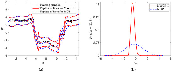
Figure 5. Fitting results of MWGP I and MGP on ${\mathcal{S}}_1$: (a) Predictions of MWGP I and MGP. Line triplets represent the mean and two standard deviation (SD) bounds; (b) predictive probability densities of MWGP I and MGP at $x=11.3$.

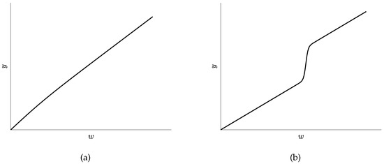
Figure 6. Warping functions obtained by MWGP I on ${\mathcal{S}}_1$: (a) The warping function learned in the first component; (b) the warping function learned in the second component.

In Table 3, the average predicted RMSEs, SDs of predicted RMSEs, p-values [52] of predicted RMSEs, and average running times for MWGP I and the other models on ${\mathcal{S}}_1,{\mathcal{S}}_2,\cdots ,{\mathcal{S}}_{10}$ are illustrated, where p-values are obtained by MWGP I and the other comparative models, respectively. The prediction accuracies of MWGP I and MGP are better than the other models due to the mixture structure, and the prediction accuracy of MWGP I is the best of all. MWGP I is superior to MGP in accuracy because of the warping function. Although the SDEPs of ${\gamma }_c^{\left(1\right)}$ and ${\gamma }_c^{\left(2\right)}$ are larger than the other parameters, the predicted results of MWGP I are accurate in ${\mathcal{S}}_1$. Thus, MWGP I is robust for the estimates of ${\gamma }_c^{\left(1\right)}$ and ${\gamma }_c^{\left(2\right)}$. The SDs of predicted RMSEs for MWGP I and the other models are small. From the p-values, the predicted RMSE of MWGP I is different from the other models, except for MGP on ${\mathcal{S}}_3$ and ${\mathcal{S}}_5$. Thus, our proposed MWGP I is effective, and it can optimize all parameters jointly.

Table 3. The average predicted RMSEs, SDs of predicted RMSEs, p-values of predicted RMSEs, and average running times (seconds) for MWGP I and the other models from over one hundred trials on synthetic datasets; the bold font represents the best results.

Model	${\mathcal{S}}_1$				${\mathcal{S}}_2$				${\mathcal{S}}_3$				${\mathcal{S}}_4$				${\mathcal{S}}_5$
	RMSE			Time	RMSE			Time	RMSE			Time	RMSE			Time	RMSE			Time
	Average	SD	p-Value		Average	SD	p-Value		Average	SD	p-Value		Average	SD	p-Value		Average	SD	p-Value
MWGP I	$\mathbf{0.1024}$	0.0312	−	$2.5916$	$\mathbf{0.0891}$	0.0641	−	$2.6589$	$\mathbf{0.3751}$	0.0543	−	$2.8216$	$\mathbf{0.0901}$	0.0394	−	$2.5175$	0.5077	0.0346	−	2.5261
MGP	$0.1442$	0.0217	0.0000	$1.9620$	$0.1142$	0.0638	0.0000	$2.5429$	$0.3792$	0.0473	0.1319	$2.5187$	$0.1331$	0.0418	0.0000	$1.9213$	$0.5178$	0.0415	0.0571	$2.0896$
WGP	$0.2507$	0.0242	0.0000	$0.2250$	$0.1694$	0.0505	0.0000	$0.2019$	$0.4168$	0.0096	0.0000	$0.2133$	$0.1417$	0.0437	0.0000	$0.2041$	$0.5569$	0.0310	0.0000	$0.1940$
GP	$0.4083$	0.0605	0.0000	$0.1637$	$0.2867$	0.0471	0.0000	$0.1581$	$0.5434$	0.0261	0.0000	$0.1661$	$0.2146$	0.0624	0.0000	$0.1590$	$0.6676$	0.0113	0.0000	$0.1714$
FNN	0.3715	0.1330	0.0000	1.9095	0.2695	0.0143	0.0000	1.6244	0.7014	0.1307	0.0000	1.7249	0.2928	0.0514	0.0000	2.4233	0.6749	0.1753	0.0000	2.1344
SVM	0.4605	0.1942	0.0000	45.236	0.3561	0.0139	0.0000	52.126	0.7901	0.1889	0.0000	39.451	0.3051	0.0539	0.0000	52.089	0.7295	0.2657	0.0000	58.141
Model	${\mathcal{S}}_6$				${\mathcal{S}}_7$				${\mathcal{S}}_8$				${\mathcal{S}}_9$				${\mathcal{S}}_{10}$
	RMSE			Time	RMSE			Time	RMSE			Time	RMSE			Time	RMSE			Time
	average	SD	p-value		average	SD	p-value		average	SD	p-value		average	SD	p-value		average	SD	p-value
MWGP I	$\mathbf{0.0807}$	0.0196	−	$2.5135$	$\mathbf{0.2869}$	0.0318	−	$2.5388$	0.2582	0.0316	−	2.8099	0.4858	0.0296	−	2.7052	$\mathbf{0.1816}$	0.0273	−	$2.3483$
MGP	$0.1248$	0.0197	0.0000	$2.4189$	$0.3028$	0.0528	0.0000	$1.9746$	0.2719	0.0372	0.0000	2.2128	0.5105	0.0343	0.0000	2.1638	$0.2090$	0.0337	0.0000	$1.8251$
WGP	$0.1702$	0.0527	0.0000	$0.2609$	$0.3250$	0.0492	0.0000	$0.2269$	0.3069	0.1058	0.0000	0.2342	0.5492	0.1279	0.0000	0.2958	$0.2709$	0.0581	0.0000	$0.2382$
GP	$0.3456$	0.0828	0.0000	$0.1688$	$0.4787$	0.0836	0.0000	$0.1654$	0.4352	0.1304	0.0000	0.1680	0.5596	0.1336	0.0000	0.2086	$0.4416$	0.0977	0.0000	$0.1601$
FNN	0.3230	0.0907	0.0000	2.0654	0.3720	0.1551	0.0000	1.8096	0.4527	0.1316	0.0000	2.2110	0.5496	0.1561	0.0000	2.1758	0.3768	0.1409	0.0000	1.6346
SVM	0.4915	0.1544	0.0000	51.590	0.5443	0.2024	0.0000	43.145	0.4958	0.1672	0.0000	55.062	0.5578	0.1736	0.0000	55.242	0.4675	0.1632	0.0000	48.347

5.3. Synthetic Datasets of MWGP II

For MWGP I, there is a local optimum in some cases. We propose MWGP II as a solution to this issue. To verify the consistency of MWGP II, we generated 6 typical synthetic datasets ${\mathcal{S}}_{11},{\mathcal{S}}_{12},\cdots ,{\mathcal{S}}_{16}$ by MGP with C = 5 and $E=2$. In ${\mathcal{S}}_{11}$, there are 750 training samples and 1500 test samples. In each dataset, samples are warped by $g(•;{\mathsf{\Omega }}_c)$. We set J = 3 and generated ${\mathsf{\Omega }}_c$ at random using a Gaussian distribution for these synthetic datasets. The main parameters of MWGP II on ${\mathcal{S}}_{11}$ are shown in Table 4. The other datasets that differ from ${\mathcal{S}}_{11}$ are listed as follows.

Table 4. The main parameters of MWGP II on ${\mathcal{S}}_{11}$.

	${\mathit{\eta }}_{\mathit{c}}$	${\mathit{\alpha }}_{\mathit{c}}^{\left(1\right)}$	${\mathit{\alpha }}_{\mathit{c}}^{\left(2\right)}$	${\left({\mathsf{\Sigma }}_{\mathit{c}}^{\left(11\right)}\right)}^{1/2}$	${\left({\mathsf{\Sigma }}_{\mathit{c}}^{\left(12\right)}\right)}^{1/2}$	${\left({\mathsf{\Sigma }}_{\mathit{c}}^{\left(21\right)}\right)}^{1/2}$	${\left({\mathsf{\Sigma }}_{\mathit{c}}^{\left(22\right)}\right)}^{1/2}$	${\mathit{\sigma }}_{\mathit{c}}$	${\mathit{\gamma }}_{\mathit{c}}^{\left(1\right)}$	${\mathit{\gamma }}_{\mathit{c}}^{\left(2\right)}$	${\mathit{\gamma }}_{\mathit{c}}^{\left(3\right)}$
$c=1$	0.2000	3.0000	3.0000	1.8974	1.5000	1.5000	1.8974	0.1414	0.1414	0.2887	1.2910
$c=2$	0.2000	10.500	10.500	2.8460	−2.1000	−2.1000	2.8460	0.0200	1.0000	2.2361	0.5000
$c=3$	0.2000	18.000	18.000	1.8974	0.0000	0.0000	1.8974	0.1414	0.4472	1.8257	1.5811
$c=4$	0.2000	25.500	25.500	2.8460	−2.1000	−2.1000	2.8460	0.0200	0.5000	0.7071	0.7071
$c=5$	0.2000	33.000	33.000	1.8974	1.5000	1.5000	1.8974	0.1414	0.2739	2.2361	1.2910

• ${\mathcal{S}}_{12}$ (a noise dataset): ${\sigma }_1={\sigma }_3={\sigma }_5=0.5000$, and ${\sigma }_2={\sigma }_4=0.1000$.
• ${\mathcal{S}}_{13}:$${\gamma }_1^{\left(1\right)}=0.2828$, ${\gamma }_2^{\left(1\right)}=2.0000$, ${\gamma }_3^{\left(1\right)}=0.8944$, ${\gamma }_4^{\left(1\right)}=0.7071$, and ${\gamma }_5^{\left(1\right)}=0.5477$.
• ${\mathcal{S}}_{14}$ (a length-scale dataset): ${\gamma }_1^{\left(2\right)}=0.2041$, ${\gamma }_2^{\left(2\right)}=1.5811$, ${\gamma }_3^{\left(2\right)}=1.2910$, ${\gamma }_4^{\left(2\right)}=0.5000$, and ${\gamma }_5^{\left(2\right)}=1.5811$.
• ${\mathcal{S}}_{15}$ (an overlapping dataset):

  $$\begin{array}{c}\hfill \begin{array}{cc}& {\mathsf{\Sigma }}_1^{1/2}=[3.0000,2.4000;2.4000,3.0000],\hfill \\ & {\mathsf{\Sigma }}_2^{1/2}=[4.5000,-3.8730;-3.8730,4.5000],\hfill \\ & {\mathsf{\Sigma }}_3^{1/2}=[3.0000,0.0000;3.0000,0.0000],\hfill \\ & {\mathsf{\Sigma }}_4^{1/2}=[4.5000,-3.8730;-3.8730,4.5000],\hfill \\ & {\mathsf{\Sigma }}_5^{1/2}=[3.0000,2.4000;2.4000,3.0000].\hfill \end{array}\end{array}$$
• ${\mathcal{S}}_{16}$ (an unbalanced dataset): ${\eta }_1=1/9$, ${\eta }_2=3/9$, ${\eta }_3=1/9$, and ${\eta }_4=3/9$, ${\eta }_5=1/9$.

The average ALLFs (approximated log-likelihood functions, i.e., values of the approximated Q-function after convergence of the SMCEM algorithm) and average running times of MWGP II and MWGP I on ${\mathcal{S}}_{11},{\mathcal{S}}_{12},\cdots ,{\mathcal{S}}_{16}$ are shown in Table 5. In these synthetic datasets, the average ALLF of MWGP II is larger than MWGP I, so MWGP II overcomes the local optimum of MWGP I. The average running time of MWGP II is longer than MWGP I since the partial CEM algorithm and the CEM algorithm are performed several times for the training of MWGP II. It can be concluded from the above discussion that our proposed MWGP II is effective.

Table 5. The average ALLFs and running times (seconds) of MWGP II and MWGP I from over one hundred trials on the synthetic datasets; the bold font represents the best results.

Model	${\mathcal{S}}_{11}$		${\mathcal{S}}_{12}$		${\mathcal{S}}_{13}$
	ALLF	Time	ALLF	Time	ALLF	Time
MWGP II	$-\mathbf{1.0867}\times {\mathbf{10}}^{\mathbf{3}}$	11.438	$-\mathbf{1.6752}\times {\mathbf{10}}^{\mathbf{3}}$	10.584	$-\mathbf{1.7330}\times {\mathbf{10}}^{\mathbf{3}}$	11.478
MWGP I	$-1.1678\times {10}^3$	5.4443	$-1.7388\times {10}^3$	3.9803	$-1.8351\times {10}^3$	5.4065
Model	${\mathcal{S}}_{14}$		${\mathcal{S}}_{15}$		${\mathcal{S}}_{16}$
	ALLF	Time	ALLF	Time	ALLF	Time
MWGP II	$-\mathbf{1.4240}\times {\mathbf{10}}^{\mathbf{3}}$	10.315	$-\mathbf{1.5961}\times {\mathbf{10}}^{\mathbf{3}}$	11.527	$-\mathbf{1.1597}\times {\mathbf{10}}^{\mathbf{3}}$	12.130
MWGP I	$-1.5726\times {10}^3$	3.9889	$-1.6786\times {10}^3$	5.5424	$-1.2283\times {10}^3$	5.7286

5.4. Toy and Motorcycle Datasets

Toy data [7,27] and motorcycle data [6,8,27] were used to test the performance of the MGP. We tested the consistency of our proposed MWGP II and MWGP I on the toy dataset ${\mathcal{S}}_{17}$ and the motorcycle dataset ${\mathcal{S}}_{18}$. ${\mathcal{S}}_{17}$ consisted of four components generated by four continuous functions, i.e.,

$$\begin{array}{c}\hfill \begin{array}{cc}& y_1=0.25x_1^2-40+\sqrt{7}ϵ,\hfill \\ & y_2=-0.0625{(x_2-18)}^2+0.5x_2+20+\sqrt{7}ϵ,\hfill \\ & y_3=0.008{(x_3-60)}^2-70+2ϵ,\hfill \\ & y_4=-sin\left(x_4\right)-6+\sqrt{2}ϵ,\hfill \end{array}\end{array}$$

where $x_1\in (0,15),$ $x_2\in (35,60),$ $x_3\in (45,80),$ $x_4\in (80,100)$ and $ϵ\sim \mathrm{N}(0,1)$, as shown in Figure 7a. In each component, there are 50 training samples and 50 test samples. We set J = 2 and C = 4 for ${\mathcal{S}}_{17}$.

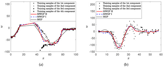
Figure 7. (a) Predictions of MWGP II, MWGP I, and MGP on ${\mathcal{S}}_{17};$ (b) predictions of MWGP II, MWGP I, and MGP on ${\mathcal{S}}_{18}$.

${\mathcal{S}}_{18}$ presents the accelerometer readings recorded at 133 moments during an experiment evaluating the effectiveness of crash helmets. In ${\mathcal{S}}_{18}$, samples belong to three components along the time axis (millisecond), i.e., $(2.4,11.4]$, $(11.4,40.4],$ and $(40.4,57.6]$, as shown in Figure 7b. We performed 7-fold cross-validation on this dataset, with the k-th fold consisting of the dataset $\{(x_n,y_n):n=7i+k,i=0,1,\cdots ,18\}$. We used 19 samples as the test set and the remaining samples as the training set. For this dataset, we set J = 2 and C = 3 for ${\mathcal{S}}_{18}$.

We compare the MWGP II, MWGP I, MGP, WGP, GP, FNN, and SVM models on ${\mathcal{S}}_{17}$ and ${\mathcal{S}}_{18}$, respectively. The average predicted RMSEs, average predicted MAEs, and average running times of these models are listed in Table 6. With these datasets, MWGP II and MWGP I are more accurate than the other models, and MWGP II is more accurate than MWGP I. The average predicted RMSE and average predicted MAE of the MGP are larger than those of a single GP and the WGP since the data in ${\mathcal{S}}_{17}$ and ${\mathcal{S}}_{18}$ are highly multimodal and non-stationary. The FNN and SVM can hardly fit ${\mathcal{S}}_{17}$ and ${\mathcal{S}}_{18}$ accurately. In Figure 7a, MWGP II and MWGP I are better than the MGP, for example on the interval $(80,100)$; in Figure 7b, MWGP II and MWGP I are better than the MGP, for example on the interval $(2.4,11.4]$. Consequently, both MWGP II and MWGP I are effective for these tasks, and MWGP II can overcome the local optimum of MWGP I at the expense of only a little time on these datasets. In summary, the preprocessing transformation is critical for MGP in the toy and motorcycle datasets.

Table 6. The average predicted RMSEs, average predicted MAEs, and average running times (seconds) of different models from over thirty trials on the toy dataset, the motorcycle dataset, and the river-flow datasets; the bold font represents the best results.

Model	${\mathcal{S}}_{17}$			${\mathcal{S}}_{18}$			${\mathcal{S}}_{19}$			${\mathcal{S}}_{20}$
	RMSE	MAE	Time	RMSE	MAE	Time	RMSE	MAE	Time	RMSE	MAE	Time
MWGP II	13.481	7.7561	6.9812	24.153	13.297	15.671	47.896	29.157	2.3341	10.425	5.5228	2.2285
MWGP I	$\mathbf{14.312}$	8.1550	$2.3733$	$\mathbf{25.987}$	14.309	$6.8800$	$\mathbf{48.171}$	29.316	$1.0935$	$\mathbf{10.668}$	5.7159	$1.0824$
MGP	14.714	8.4912	1.6331	26.370	14.351	4.4129	49.060	30.075	0.7358	11.071	6.0772	0.6139
WGP	$14.772$	8.4834	$0.1231$	$29.277$	16.579	$0.4211$	$49.411$	30.391	$0.0824$	$11.654$	6.5137	$0.0806$
GP	$20.387$	13.322	$0.1070$	$26.700$	14.725	$0.3186$	$55.466$	35.323	$0.0703$	$14.174$	8.7933	$0.0645$
FNN	18.004	11.974	1.6293	30.359	17.213	16.433	49.588	30.514	1.2033	11.669	6.5154	1.1592
SVM	17.267	11.445	46.223	29.782	16.885	182.67	54.627	34.917	25.333	12.780	7.4816	23.858
Model	${\mathcal{S}}_{21}$			${\mathcal{S}}_{22}$			${\mathcal{S}}_{23}$			${\mathcal{S}}_{24}$
	RMSE	MAE	Time	RMSE	MAE	Time	RMSE	MAE	Time	RMSE	MAE	Time
MWGP II	4.5938	3.7556	2.2943	14.266	8.6631	2.4118	16.617	10.885	2.2389	31.171	22.483	2.2581
MWGP I	4.6721	3.8321	1.0644	14.570	8.9534	1.1831	16.727	10.988	1.1016	$\mathbf{31.536}$	22.814	$1.1268$
MGP	5.1759	4.3327	0.5734	14.924	9.2859	0.5911	16.814	11.067	0.7345	34.575	26.257	0.7646
WGP	4.7084	3.8626	0.0673	15.318	9.6578	0.0939	16.728	10.990	0.0886	$32.428$	23.877	$0.0819$
GP	5.6274	4.6852	0.0587	16.161	10.527	0.0718	17.043	11.302	0.0711	$34.813$	26.416	$0.0755$
FNN	4.7079	3.8629	1.1525	15.599	9.9261	1.3947	16.738	10.996	1.1650	32.666	24.093	1.1725
SVM	4.8446	3.9841	19.240	16.353	10.673	26.039	17.415	11.579	23.659	33.163	24.552	23.745
Model	${\mathcal{S}}_{25}$			${\mathcal{S}}_{26}$			${\mathcal{S}}_{27}$			${\mathcal{S}}_{28}$
	RMSE	MAE	Time	RMSE	MAE	Time	RMSE	MAE	Time	RMSE	MAE	Time
MWGP II	27.736	19.675	2.4640	30.696	22.095	2.4040	50.497	31.265	2.2823	33.789	24.613	2.2461
MWGP I	$\mathbf{27.776}$	19.702	$1.2057$	30.708	22.121	1.1113	50.502	31.283	1.1090	33.792	24.624	1.0795
MGP	28.053	20.015	0.7480	32.061	23.216	0.7923	52.317	32.837	0.7065	34.529	25.277	0.7084
WGP	$27.785$	19.719	$0.0991$	30.712	22.128	0.0909	50.712	31.415	0.0857	34.004	24.858	0.0826
GP	$28.310$	20.263	$0.0762$	32.803	23.871	0.0756	52.994	33.478	0.0745	35.276	26.064	0.0738
FNN	27.921	19.998	1.1907	30.727	22.141	1.1980	50.603	31.357	1.1813	34.163	25.040	1.1099
SVM	28.098	20.068	24.062	31.812	22.844	27.023	52.920	33.432	26.387	35.072	25.821	20.228

5.5. River-flow Datasets

We conducted experiments on ten river-flow datasets ${\mathcal{S}}_{19},{\mathcal{S}}_{20},\cdots ,{\mathcal{S}}_{28}$ to verify the consistency of our proposed MWGP II and MWGP I [53]. In each dataset, about 40 years (i.e., from 1920 to 1960) of monthly river flow for rivers in the USA (such as the Current River, the Mad River, the Madison River, and the Mackenzie River) were recorded. There are approximately 155 training samples and 313 test samples in each dataset. For river-flow datasets, there is minimal correlation between prediction accuracy and the value of C. We set J = 2 and C = 4 for these datasets.

For comparison, MWGP II, MWGP I, MGP, WGP, GP, FNN, and SVM are considered in ${\mathcal{S}}_{19},{\mathcal{S}}_{20},\cdots ,{\mathcal{S}}_{28}$, respectively. The average predicted RMSEs (cubic meters/second), average predicted MAEs, and average running times of these models are recorded in Table 6. From this table, MWGP II and MWGP I are smaller than the other models in terms of the average predicted RMSE and average predicted MAE, and the average predicted RMSE and average predicted MAE of MWGP II are smaller than those of MWGP I. Although MWGP I has the same accuracy as MWGP II in ${\mathcal{S}}_{25},{\mathcal{S}}_{26},\cdots ,{\mathcal{S}}_{28}$, it is more efficient than MWGP II. Based on the analysis above, our proposed MWGP II and MWGP I are effective for processing the river-flow datasets, and demonstrate that the nonlinear transformation is useful for this type of data. Additionally, MWGP II can overcome the local optimum of MWGP I at a minimal computational cost on some datasets.

6. Conclusions and Discussion

In this paper, we demonstrate that the MWGP model is a valuable generalization of the MGP and WGP models, and it is well suited for solving non-stationary probabilistic regression. From another point of view, the standard preprocessing transformation in MWGP can be learned adaptively and improved upon. We show that simultaneous split and merge operations are able to eliminate the component differences between the two regions to avoid the local optimum of the CEM algorithm for MWGP. Experimental results on synthetic and real-world datasets show that our proposed MWGP trained by the CEM algorithm as well as MWGP trained by the SMCEM algorithm are effective.

For MWGP, the actual number of WGP components is generally difficult to learn due to the correlation among outputs. In future work, we will focus on learning C for MWGP. Moreover, for probabilistic regression models, there are likely outliers in the observations that deviate significantly from the other samples. We will consider the robustness for MWGP based on the robustness of the MGP.

Appendix A.1. The Derivation of the Q-Function and Details of the Approximated MAP Principle

Denote $g({\mathbf{w}}_c;{\mathsf{\Omega }}_c)=\left[g(w_n;{\mathsf{\Omega }}_c)|{\mathbf{z}}_n={\mathbf{e}}_c;n=1,2,\cdots ,N\right]$ as the $N_c\times 1$ function vector of the c-th component, ${\mathbf{K}}_c=\left[K({\mathbf{x}}_n,{\mathbf{x}}_{\tilde{n}};{\mathsf{\gamma }}_c)\right|{\mathbf{z}}_n={\mathbf{z}}_{\tilde{n}}={\mathbf{e}}_c;n,\tilde{n}=1,2,\cdots ,N]$ as the $N_c\times N_c$ covariance matrix of the c-th component, and ${\sum }_{n=1}^{N_c}ln\partial g(w_n;{\mathsf{\Omega }}_c)/\partial w_n$ as a Jacobian term. The total log-likelihood function of MWGP is given by

$$\begin{array}{cc}\hfill \mathrm{L}(\mathsf{\Phi },\mathbf{Z})=& lnp(\mathcal{D},\mathbf{Z}|\mathsf{\Phi })={\sum }_{c=1}^C{\mathrm{L}}_c({\mathsf{\Phi }}_c,\mathbf{Z})\hfill \\ \hfill =& {\sum }_{c=1}^C\left\{{\sum }_{n=1}^N{z}_{nc}\left[ln{\eta }_c+lnp\left({\mathbf{x}}_n\right|{\mathbf{z}}_n={\mathbf{e}}_c)\right]+lnp\left({\mathbf{w}}_c\right|{\mathbf{X}}_c,{\mathsf{\theta }}_c,{\mathsf{\Omega }}_c)\right\},\hfill \end{array}$$

(A1)

where $lnp\left({\mathbf{w}}_c\right|{\mathbf{X}}_c,{\mathsf{\theta }}_c,{\mathsf{\Omega }}_c)$ is the log-likelihood function of the c-th WGP given by

$$\begin{array}{c}\hfill \begin{array}{cc}\hfill lnp\left({\mathbf{w}}_c\right|{\mathbf{X}}_c,{\mathsf{\theta }}_c,{\mathsf{\Omega }}_c)=& -[N_{c}ln2\pi +g{({\mathbf{w}}_c;{\mathsf{\Omega }}_c)}^{\mathrm{T}}{\left({\mathbf{K}}_c+{\sigma }_c^2{\mathbf{I}}_{{\mathit{N}}_{\mathit{c}}}\right)}^{-1}g({\mathbf{w}}_c;{\mathsf{\Omega }}_c)\hfill \\ & +ln|{\mathbf{K}}_c+{\sigma }_c^2{\mathbf{I}}_{{\mathit{N}}_{\mathit{c}}}\left|\right]/2+{\sum }_{n=1}^{N_c}ln\partial g(w_n;{\mathsf{\Omega }}_c)/\partial w_n.\hfill \end{array}\end{array}$$

The Q-function of the conventional EM algorithm of MWGP is obtained by the expectation of Equation (A1) with respect to $\mathbf{Z}:$

$$\begin{array}{cc}\hfill Q\left(\mathsf{\Phi }\right|{\mathsf{\Phi }}^{(r-1)})& ={\mathbb{E}}_{\mathbf{Z}}\left[\mathrm{L}(\mathsf{\Phi },\mathbf{Z})|\mathcal{D},{\mathsf{\Phi }}^{(r-1)}\right]={\sum }_{\mathbf{Z}}P\left(\mathbf{Z}\right|\mathcal{D},{\mathsf{\Phi }}^{(r-1)})\mathrm{L}(\mathsf{\Phi },\mathbf{Z}).\hfill \end{array}$$

(A2)

The posterior probability $P\left({\mathbf{z}}_n\right|{\mathbf{x}}_n,w_n,{\mathsf{\Phi }}^{\left(r\right)})$ is calculated by

$$\begin{array}{cc}\hfill P\left({\mathbf{z}}_n\right|{\mathbf{x}}_n,w_n,{\mathsf{\Phi }}^{\left(r\right)})\propto & p({\mathbf{x}}_n,w_n,{\mathbf{z}}_n|{\mathsf{\Phi }}^{\left(r\right)})\hfill \\ \hfill =& P\left({\mathbf{z}}_n\right|{\mathsf{\Phi }}^{\left(r\right)})p\left({\mathbf{x}}_n\right|{\mathbf{z}}_n,{\mathsf{\Phi }}^{\left(r\right)})p\left(w_n\right|{\mathbf{x}}_n,{\mathbf{z}}_n,{\mathsf{\Phi }}^{\left(r\right)})\hfill \\ \hfill =& P\left({\mathbf{z}}_n\right|{\mathsf{\Phi }}^{\left(r\right)})p\left({\mathbf{x}}_n\right|{\mathbf{z}}_n,{\mathsf{\Phi }}^{\left(r\right)})p\left(y_n\right|{\mathbf{x}}_n,{\mathbf{z}}_n,{\mathsf{\Phi }}^{\left(r\right)})\hfill \\ \hfill =& P\left({\mathbf{z}}_n\right|{\mathsf{\Phi }}^{\left(r\right)})p\left({\mathbf{x}}_n\right|{\mathbf{z}}_n,{\mathsf{\Phi }}^{\left(r\right)})\hfill \\ \hfill & •p\left(g(w_n;{\mathsf{\Omega }}^{\left(r\right)})\right|{\mathbf{x}}_n,{\mathbf{z}}_n,{\mathsf{\Phi }}^{\left(r\right)})\partial g(w_n;{\mathsf{\Omega }}^{\left(r\right)})/\partial w_n,\hfill \end{array}$$

(A3)

where $\partial g(w_n;{\mathsf{\Omega }}^{\left(r\right)})/\partial w_n$ is the Jacobian term. Since the number of $\mathbf{Z}$ is $C^N$, the time complexity of calculating Equation (A2) is $O\left(C^N\right)$. Thus, the classification approximation is adopted for calculating Equation (A2), and then we obtain the approximated Q-function for the CEM algorithm:

$$\begin{array}{cc}\hfill \mathrm{L}(\mathsf{\Phi },{\mathbf{Z}}^{\left(r\right)})& ={\sum }_{c=1}^C{\mathrm{L}}_c({\mathsf{\Phi }}_c,{\mathbf{Z}}^{\left(r\right)}),\hfill \end{array}$$

(A4)

where ${\mathbf{Z}}^{\left(r\right)}$ is calculated by an approximation of the MAP method, i.e., ${\mathbf{Z}}^{\left(r\right)}={argmax}_{\mathbf{Z}}P\left(\mathbf{Z}\right|\mathcal{D},{\mathsf{\Phi }}^{\left(r\right)})$:

$$\begin{array}{cc}\hfill {\mathbf{z}}_n^{\left(r\right)}=& {argmax}_{{\mathbf{z}}_n}P\left({\mathbf{z}}_n\right|{\mathbf{x}}_n,w_n,{\mathsf{\Phi }}^{\left(r\right)})\hfill \\ \hfill =& {argmax}_{{\mathbf{z}}_n}P\left({\mathbf{z}}_n\right|{\mathsf{\Phi }}^{\left(r\right)})p\left({\mathbf{x}}_n\right|{\mathbf{z}}_n,{\mathsf{\Phi }}^{\left(r\right)})\hfill \\ \hfill & •p\left(g(w_n;{\mathsf{\Omega }}^{\left(r\right)})\right|{\mathbf{x}}_n,{\mathbf{z}}_n,{\mathsf{\Phi }}^{\left(r\right)})\partial g(w_n;{\mathsf{\Omega }}^{\left(r\right)})/\partial w_n.\hfill \end{array}$$

(A5)

In Equation (A5), $P\left({\mathbf{z}}_n\right|{\mathbf{x}}_n,w_n,{\mathsf{\Phi }}^{\left(r\right)})$ is derived by Equation (A3).

Appendix A.2. Details for Maximizing the Approximated Q-Function

Parameters ${\mathsf{\theta }}_c$ and ${\mathsf{\Omega }}_c$ are updated jointly by the conjugated gradient method inherited by training the WGP.

Parameters ${\eta }_c,$${\mathsf{\alpha }}_c$, and ${\mathsf{\Sigma }}_c$ are solved analytically as follows. By adopting the Lagrange multiplier method when ${\sum }_{c=1}^C{\eta }_c=1$, we have

$${\eta }_c=N_c/{\sum }_{c=1}^C{N}_c.$$

Let $\partial \mathrm{L}(\mathsf{\Phi },{\mathbf{Z}}^{(r-1)})/\partial {\mathsf{\alpha }}_c$ = 0 and $\partial \mathrm{L}(\mathsf{\Phi },{\mathbf{Z}}^{(r-1)})/\partial {\mathsf{\Sigma }}_c$ = 0. Then, we have

$$\begin{array}{c}{\mathsf{\alpha }}_c={\sum }_{n=1}^N{z}_{nc}{\mathbf{x}}_n/N_c,\\ {\mathsf{\Sigma }}_c={\sum }_{n=1}^N{z}_{nc}({\mathbf{x}}_n-{\mathsf{\alpha }}_c){({\mathbf{x}}_n-{\mathsf{\alpha }}_c)}^{\mathrm{T}}/N_c.\end{array}$$

Appendix B.1. Details of Maximizing the Approximated Q-Function of the Partial CEM Algorithm

The approximated Q-function Equation (A4) is equal to

$$\begin{array}{cc}\hfill \mathrm{L}(\mathsf{\Phi },{\mathbf{Z}}^{\left(r\right)})=& {\sum }_{c=u,s,t}{\mathrm{L}}_c({\mathsf{\Phi }}_c,{\mathbf{Z}}^{\left(r\right)})+{\sum }_{c\ne u,s,t}{\mathrm{L}}_c({\mathsf{\Phi }}_c,{\mathbf{Z}}^{\left(r\right)}),\hfill \end{array}$$

where the first three terms, i.e., ${\sum }_{c=u,s,t}{\mathrm{L}}_c({\mathsf{\Phi }}_c,{\mathbf{Z}}^{\left(r\right)}),$ are only maximized for the partial CEM algorithm. The details for maximizing ${\sum }_{c=u,s,t}{\mathrm{L}}_c({\mathsf{\Phi }}_c,{\mathbf{Z}}^{\left(r\right)})$ are described in Appendix A.2.

Appendix B.2. Details of the Approximated MAP Principle of the Partial CEM Algorithm

When ${\mathbf{z}}_n^{(r-1)}={\mathbf{e}}_{c=u,s,t}$, ${\mathbf{z}}_n^{\left(r\right)}$ is obtained by the approximated MAP method:

$$\begin{array}{cc}\hfill {\mathbf{z}}_n^{\left(r\right)}=& {argmax}_{{\mathbf{z}}_n\in \left\{{\mathbf{e}}_{c=u,s,t}\right\}}P\left({\mathbf{z}}_n\right|{\mathbf{x}}_n,w_n,{\mathsf{\Phi }}_c^{\left(r\right)})\hfill \\ \hfill =& {argmax}_{{\mathbf{z}}_n\in \left\{{\mathbf{e}}_{c=u,s,t}\right\}}P({\mathbf{z}}_n={\mathbf{e}}_c|{\mathsf{\Phi }}_c^{\left(r\right)})p\left({\mathbf{x}}_n\right|{\mathbf{z}}_n={\mathbf{e}}_c,{\mathsf{\Phi }}_c^{\left(r\right)})\hfill \\ \hfill & •p\left(g(w_n;{\mathsf{\Omega }}_c^{\left(r\right)})\right|{\mathbf{x}}_n,{\mathbf{z}}_n={\mathbf{e}}_c,{\mathsf{\Phi }}_c^{\left(r\right)})\partial g(w_n;{\mathsf{\Omega }}_c^{\left(r\right)})/\partial w_n,\hfill \end{array}$$

where $P\left({\mathbf{z}}_n\right|{\mathbf{x}}_n,w_n,{\mathsf{\Phi }}_c^{\left(r\right)})$ is derived by Equation (A3).

References

- Yuksel, S.E.; Wilson, J.N.; Gader, P.D. Twenty years of mixture of experts. IEEE Trans. Neural Netw. Learn. Syst. 2012, 23, 1177–1193. [Google Scholar] [CrossRef]
- Jordan, M.I.; Jacobs, R.A. Hierarchies mixtures of experts and the EM algorithm. Neural Comput. 1994, 6, 181–214. [Google Scholar] [CrossRef]
- Lima, C.A.M.; Coelho, A.L.V.; Zuben, F.J.V. Hybridizing mixtures of experts with support vector machines: Investigation into nonlinear dynamic systems identification. Inf. Sci. 2007, 177, 2049–2074. [Google Scholar] [CrossRef]
- Tresp, V. Mixtures of Gaussian processes. In Proceedings of the Advances in Neural Information Processing Systems (NIPS), Denver, CO, USA, 1 January 2000; Volume 13, pp. 654–660. [Google Scholar]
- Dempster, A.P.; Laird, N.M.; Rubin, D.B. Maximum likelihood from incomplete data via the EM algorithm. J. R. Stat. Soc. Ser. B Methodol. 1977, 39, 1–38. [Google Scholar]
- Rasmussen, C.E.; Ghahramani, Z. Infinite mixture of Gaussian process experts. In Proceedings of the Advances in Neural Information Processing Systems (NIPS), Vancouver, BC, Canada, 9–14 December 2002; Volume 2, pp. 881–888. [Google Scholar]
- Meeds, E.; Osindero, S. An alternative infinite mixture of Gaussian process experts. In Proceedings of the Advances in Neural Information Processing Systems (NIPS), Vancouver, BC, Canada, 4–7 December 2005; Volume 18, pp. 883–896. [Google Scholar]
- Yuan, C.; Neubauer, C. Variational mixture of Gaussian process experts. In Proceedings of the Advances in Neural Information Processing Systems (NIPS), Vancouver, BC, Canada, 8–11 December 2008; Volume 21, pp. 1897–1904. [Google Scholar]
- Brahim-Belhouari, S.; Bermak, A. Gaussian process for nonstationary time series prediction. Comput. Stat. Data Anal. 2004, 47, 705–712. [Google Scholar] [CrossRef]
- Pérez-Cruz, F.; Vaerenbergh, S.V.; Murillo-Fuentes, J.J.; Lázaro-Gredilla, M.; Santamaría, I. Gaussian processes for nonlinear signal processing: An overview of recent advances. IEEE Signal Process. Mag. 2013, 30, 40–50. [Google Scholar] [CrossRef]
- Rasmussen, C.E.; Williams, C.K.I. Gaussian Process for Machine Learning; MIT Press: Cambridge, MA, USA, 2006; Chapter 2. [Google Scholar]
- MacKay, D.J.C. Introduction to Gaussian processes. NATO ASI Ser. F Comput. Syst. Sci. 1998, 168, 133–166. [Google Scholar]
- Xu, Z.; Guo, Y.; Saleh, J.H. VisPro: A prognostic SqueezeNet and non-stationary Gaussian process approach for remaining useful life prediction with uncertainty quantification. Neural Comput. Appl. 2022, 34, 14683–14698. [Google Scholar] [CrossRef]
- Heinonen, M.; Mannerström, H.; Rousu, J.; Kaski, S.; Lähdesmäki, H. Non-stationary Gaussian process regression with hamiltonian monte carlo. In Proceedings of the Machine Learning Research, Cadiz, Spain, 9–11 May 2016; Volume 51, pp. 732–740. [Google Scholar]
- Wang, Y.; Chaib-draa, B. Bayesian inference for time-varying applications: Particle-based Gaussian process approaches. Neurocomputing 2017, 238, 351–364. [Google Scholar] [CrossRef]
- Rhode, S. Non-stationary Gaussian process regression applied in validation of vehicle dynamics models. Eng. Appl. Artif. Intell. 2020, 93, 103716. [Google Scholar] [CrossRef]
- Sun, S.; Xu, X. Variational inference for infinite mixtures of Gaussian processes with applications to traffic flow prediction. IEEE Trans. Intell. Transp. Syst. 2010, 12, 466–475. [Google Scholar] [CrossRef]
- Jeon, Y.; Hwang, G. Bayesian mixture of gaussian processes for data association problem. Pattern Recognit. 2022, 127, 108592. [Google Scholar] [CrossRef]
- Li, T.; Ma, J. Attention mechanism based mixture of Gaussian processes. Pattern Recognit. Lett. 2022, 161, 130–136. [Google Scholar] [CrossRef]
- Kim, S.; Kim, J. Efficient clustering for continuous occupancy mapping using a mixture of Gaussian processes. Sensors 2022, 22, 6832. [Google Scholar] [CrossRef]
- Tayal, A.; Poupart, P.; Li, Y. Hierarchical double Dirichlet process mixture of Gaussian processes. In Proceedings of the 26th AAAI Conference on Artificial Intelligence (AAAI), Toronto, ON, Canada, 22–26 July 2012; pp. 1126–1133. [Google Scholar]
- Sun, S. Infinite mixtures of multivariate Gaussian processes. In Proceedings of the International Conference on Machine Learning and Cybernetics (ICMLC), Tianjin, China, 14–17 July 2013; pp. 1011–1016. [Google Scholar]
- Kastner, M. Monte Carlo methods in statistical physics: Mathematical foundations and strategies. Commun. Nonlinear Sci. Numer. Simul. 2010, 15, 1589–1602. [Google Scholar] [CrossRef]
- Khodadadian, A.; Parvizi, M.; Teshnehlab, M.; Heitzinger, C. Rational design of field-effect sensors using partial differential equations, Bayesian inversion, and artificial neural networks. Sensors 2022, 22, 4785. [Google Scholar] [CrossRef] [PubMed]
- Noii, N.; Khodadadian, A.; Ulloa, J.; Aldakheel, F.; Wick, T.; François, S.; Wriggers, P. Bayesian inversion with open-source codes for various one-dimensional model problems in computational mechanics. Arch. Comput. Methods Eng. 2022, 29, 4285–4318. [Google Scholar] [CrossRef]
- Ross, J.C.; Dy, J.G. Nonparametric mixture of Gaussian processes with constraints. In Proceedings of the 30th International Conference on Machine Learning (ICML), Atlanta, GA, USA, 17–19 June 2013; pp. 1346–1354. [Google Scholar]
- Yang, Y.; Ma, J. An efficient EM approach to parameter learning of the mixture of Gaussian processes. In Proceedings of the Advances in International Symposium on Neural Networks (ISNN), Guilin, China, 29 May–1 June 2011; Volume 6676, pp. 165–174. [Google Scholar]
- Chen, Z.; Ma, J.; Zhou, Y. A precise hard-cut EM algorithm for mixtures of Gaussian processes. In Proceedings of the 10th International Conference on Intelligent Computing (ICIC), Taiyuan, China, 3–6 August 2014; Volume 8589, pp. 68–75. [Google Scholar]
- Celeux, G.; Govaert, G. A classification EM algorithm for clustering and two stochastic versions. Comput. Stat. Data Anal. 1992, 14, 315–332. [Google Scholar] [CrossRef]
- Wu, D.; Chen, Z.; Ma, J. An MCMC based EM algorithm for mixtures of Gaussian processes. In Proceedings of the Advances in International Symposium on Neural Networks (ISNN), Jeju, Republic of Korea, 15–18 October 2015; Volume 9377, pp. 327–334. [Google Scholar]
- Wu, D.; Ma, J. An effective EM algorithm for mixtures of Gaussian processes via the MCMC sampling and approximation. Neurocomputing 2019, 331, 366–374. [Google Scholar] [CrossRef]
- Ma, J.; Xu, L.; Jordan, M.I. Asymptotic convergence rate of the EM algorithm for Gaussian mixtures. Neural Comput. 2000, 12, 2881–2907. [Google Scholar] [CrossRef]
- Zhao, L.; Chen, Z.; Ma, J. An effective model selection criterion for mixtures of Gaussian processes. In Proceedings of the Advances in Neural Networks-ISNN, Jeju, Republic of Korea, 15–18 October 2015; Volume 9377, pp. 345–354. [Google Scholar]
- Ueda, N.; Nakano, R.; Ghahramani, Z.; Hinton, G.E. SMEM algorithm for mixture models. Adv. Neural Inf. Process. Syst. 1998, 11, 599–605. [Google Scholar] [CrossRef] [PubMed]
- Li, Y.; Li, L. A novel split and merge EM algorithm for Gaussian mixture model. In Proceedings of the International Conference on Natural Computation (ICNC), Tianjin, China, 14–16 August 2009; pp. 479–483. [Google Scholar]
- Zhang, Z.; Chen, C.; Sun, J.; Chan, K.L. EM algorithms for Gaussian mixtures with split-and-merge operation. Pattern Recognit. 2003, 36, 1973–1983. [Google Scholar] [CrossRef]
- Zhao, L.; Ma, J. A dynamic model selection algorithm for mixtures of Gaussian processes. In Proceedings of the IEEE 13th International Conference on Signal Processing (ICSP), Chengdu, China, 6–10 November 2016; pp. 1095–1099. [Google Scholar]
- Li, T.; Wu, D.; Ma, J. Mixture of robust Gaussian processes and its hard-cut EM algorithm with variational bounding approximation. Neurocomputing 2021, 452, 224–238. [Google Scholar] [CrossRef]
- Snelson, E.; Rasmussen, C.E.; Ghahramani, Z. Warped Gaussian processes. Adv. Neural Inf. Process. Syst. 2003, 16, 337–344. [Google Scholar]
- Schmidt, M.N. Function factorization using warped Gaussian processes. In Proceedings of the 26th International Conference on Machine Learning (ICML), Montreal, QC, Canada, 14–18 June 2009; pp. 921–928. [Google Scholar]
- Lázaro-Gredilla, M. Bayesian warped Gaussian processes. Adv. Neural Inf. Process. Syst. 2012, 25, 6995–7004. [Google Scholar]
- Rios, G.; Tobar, F. Compositionally-warped Gaussian processes. Neural Netw. 2019, 118, 235–246. [Google Scholar] [CrossRef]
- Zhang, Y.; Yeung, D.Y. Multi-task warped Gaussian process for personalized age estimation. In Proceedings of the IEEE Computer Society Conference on Computer Vision and Pattern Recognition (CVPR), San Francisco, CA, USA, 13–18 June 2010; pp. 2622–2629. [Google Scholar]
- Wiebe, J.; Cecílio, I.; Dunlop, J.; Misener, R. A robust approach to warped Gaussian process-constrained optimization. Math. Program. 2022, 196, 805–839. [Google Scholar] [CrossRef]
- Mateo-Sanchis, A.; Muñoz-Marí, J.; Pérez-Suay, A.; Camps-Valls, G. Warped Gaussian processes in remote sensing parameter estimation and causal inference. IEEE Geosci. Remote Sens. Lett. 2018, 15, 1647–1651. [Google Scholar] [CrossRef]
- Jadidi, M.G.; Miró, J.V.; Dissanayake, G. Warped Gaussian processes occupancy mapping with uncertain inputs. IEEE Robot. Autom. Lett. 2017, 2, 680–687. [Google Scholar] [CrossRef]
- Kou, P.; Liang, D.; Gao, F.; Gao, L. Probabilistic wind power forecasting with online model selection and warped Gaussian process. Energy Convers. Manag. 2014, 84, 649–663. [Google Scholar] [CrossRef]
- Gonçalves, I.G.; Echer, E.; Frigo, E. Sunspot cycle prediction using warped Gaussian process regression. Adv. Space Res. 2020, 65, 677–683. [Google Scholar] [CrossRef]
- Rasmussen, C.E.; Nickisch, H. Gaussian processes for machine learning (GPML) toolbox. J. Mach. Learn. Res. 2010, 11, 3011–3015. [Google Scholar]
- Svozil, D.; Kvasnicka, V.; Pospichal, J. Introduction to multi-layer feedforward neural networks. Chemom. Intell. Lab. Syst. 1997, 39, 43–62. [Google Scholar] [CrossRef]
- Chang, C.C.; Lin, C.J. LIBSVM: A library for support vector machines. ACM Trans. Intell. Syst. Technol. 2011, 2, 27. [Google Scholar] [CrossRef]
- Derrac, J.; García, S.; Molina, D.; Herrera, F. A practical tutorial on the use of nonparametric statistical tests as a methodology for comparing evolutionary and swarm intelligence algorithms. Swarm Evol. Comput. 2011, 1, 3–18. [Google Scholar] [CrossRef]
- Mcleod, A.I. Parsimony, model adequacy and periodic correlation in forecasting time series. Int. Stat. Rev. 1993, 61, 387–393. [Google Scholar] [CrossRef]
Disclaimer/Publisher’s Note: The statements, opinions and data contained in all publications are solely those of the individual author(s) and contributor(s) and not of MDPI and/or the editor(s). MDPI and/or the editor(s) disclaim responsibility for any injury to people or property resulting from any ideas, methods, instructions or products referred to in the content. |
© 2023 by the authors. Licensee MDPI, Basel, Switzerland. This article is an open access article distributed under the terms and conditions of the Creative Commons Attribution (CC BY) license (https://creativecommons.org/licenses/by/4.0/).