Computational Human Nasal Reconstruction Based on Facial Landmarks

Abstract

This research presented a mathematical-based approach to the computational reconstruction of the human nose through images with anthropometric characteristics. The nasal baselines, which were generated from facial aesthetic subunits combined with the facial landmarks, were reconstructed using interpolation and Mesh adaptive direct search algorithms to generate points that would serve as the support for the layer-by-layer reconstruction. The approach is proposed as the basis for nasal reconstruction in aesthetics or forensics rather than focusing on the applications of image processing or deep learning. A mathematical model for the computational reconstruction was built, and then volunteers were the subjects of nasal reconstruction experiments. The validations based on the area errors—which are based on four samples and eight sub-regions with different values depending on the regions C₁, C₂, and C₃ and nasal shapes of the volunteers—were measured to prove the results of the mathematical model. Evaluations have demonstrated that the computer-reconstructed noses fit the original ones in shape and with minimum area errors. This study describes a computational reconstruction based on a mathematical approach directly to facial anthropometric landmarks to reconstruct the nasal shape.

1. Introduction

Every person has unique characteristics that become their identifying features in society. Identification cards or passports may be used to identify them when fatal accidents occur. These identifying features include fingerprints, dental features, soft tissue features such as scars and birthmarks, deoxyribonucleic acid (DNA), and facial anthropometrics [1]. Facial anthropometrics, in addition to identification purposes, can be used as the basis for forensic reconstruction: they are the point clouds from the 3D scan devices, the computer tomography scan (CT scan) data, and the facial landmarks [2]. Facial anthropometry is used in many different fields, such as plastic surgery, facial reconstruction, protective clothing design, and emotion recognition. Classical facial reconstruction experiments were conducted by implementing the survey, measurement, and statistical methods with consideration for the skull as the starting point (i.e., craniofacial reconstruction or CFR). The CFR only approximates the face rather than accurately reconstructing all facial features, as the skull does not contain much information about the soft tissues that envelop it [1]. Classical CFR methods include sketching performed by forensic anthropologists and based on age and sex; George’s method, which uses the average thickness information of soft tissues and the relationship between it and the skull to approximately reconstruct the human head; and the three-dimensional graphical CFR method that implements George’s method for analyzing, computationally synthesizing and reconstructing [2]. The manual methods of measurement and reconstruction are time-consuming and less flexible than the computer-based methods [2]; moreover, the computer-based implementation (in particular, through side view images or CT scans) troubleshoots its manual counterparts’ problems, such as the elastic deformation of the skin and the need for specific measuring instruments, and avoids direct contact with the patient’s face [2,3,4]. Facial data can be acquired by using scan devices to obtain the points and contours, as mentioned previously [2,5]. Likewise, it is possible to use combinations of image processing, interpolation, and machine learning algorithms to extract facial data from the images of the facial reconstruction alone [6,7,8,9]. For instance, Zhang, Yu, et al. [5] used a multi-layer deformation method for an anatomy-based reconstruction whose facial graphical models’ expressions are changeable with a suitable deformation of the skin. The facial anthropometric features were acquired by using a laser scanner and mapping the reflectance images into the three-dimensional model. The whole process of reconstruction took 15 min [5]. Choi, Jongmoo, et al. [6] introduced a procedure containing sequential processes from poses and anchor points detection, facial landmarks detection, to the deformation/wrapping of a three-dimensional reference face with respect to the coordinates of the mapped landmarks extracted from a particular person’s images. Choi, Jongmoo et al.’s work can be implemented for both single and multiple views; however, they demonstrated that the implementation for a single view caused more distortion of the nose on the 3D model than the multiple views synthesized by their sparse reconstruction method [10,11]. A study demonstrating an effective reconstruction from a single image of the human face [12] presented its approach of image shading information and generic shaping to acquire the facial features (i.e., the depth of points) that are considered the basis for a reference head deformation according to the extracted depth of the image. In a separate study [13], the authors pointed out that the nose was the most attractive part of the face. Thus, studies on plastic surgery are relevant, and there are many aspects of plastic surgery that require further research. Three-dimensional reconstruction studies supporting clinical diagnosis and rhinoplasty. For the past few decades, generating human prostheses, especially facial prostheses, has required a lot of time, money, effort, skill, and a high degree of precision. The authors of another study [14] discussed the process of reconstructing prosthetics for patients with large jaw defects using digital technology for modeling and generating the prosthetics using a 3D printer. In a different study [15], the authors argued that the facial reconstruction of skin cancer patients needs to ensure personalized medicine. However, the authors only proposed a plan based on 607 patients who had post-surgery facial reconstructions to reduce their risk of complications. For patients with cancer or other diseases undergoing endoscopic skull base surgery, quality-of-life (QOL) parameters are important. Therefore, facial reconstructions through plastic surgery help patients with anterior cranial base malignancies preserve or improve their QOL [16]. Currently, facial reconstructions of patients with empty nose syndrome (ENS) have yielded satisfactory results compared with other methods [17]. Some studies [18,19] have proposed the digital reconstruction of body parts, such as the nasal airways using modeling from CT scan images and then the creation of these parts through 3D printing. Through the digital model, the analysis and computation of parameters such as pressure, velocity, and turbulent kinetic energy (TKE) can be compared with other models. Additionally, the study [20] showed that there was tissue displacement and hypoplasia for patients with cleft lip repair. Therefore, the authors proposed 3D-printed autologous cartilage rhinoplasty to reconstruct the nasal shape. In the study [21], virtual 3D skull reconstruction from neuroanatomical tomography and specimens from the Brazilian Albian Euraxemys essweini (Pleurodira, Euraxemydidae) were described. The procedures were non-destructive technology that allowed researchers to take a closer look at the internal structure to enhance the information. The reconstruction process often uses digital sculpting software to create high-resolution 3D data [15]. Computational reconstruction creates quality and efficiency that help reduce costs for the patient and overcome the disadvantages of other reconstruction methods. According to [2,10,11] presented in their work, the reconstructed 3D graphical human face models depend on the transformation of the reference heads; thus, it requires both facial anthropometric features and the computational deformation of the skin surface layer when applying a dataset of specific faces to induce shape transformations on reference heads. Our approach, which implemented basic and modified interpolation algorithms on human facial landmarks information (i.e., their coordinates relative to a specific reference system), does not require the deformation of the graphical anthropometric reference head surface. The landmarks are in Cartesian coordinates with three values of x, y, and z gathered from images taken from the frontal and lateral views of each volunteer.

Several studies show that many people were not satisfied with the parts of their faces. Additionally, there are also different face aesthetics that are the harmonization of the parts of the face as well as the structure of the face. The nose is an impressive and important part of the face. To identify, reconstruct, and perform cosmetic surgery, doctors need to understand the nasal shape as well as the relationship between the nose and the face. The reconstruction of the nose from its anthropometric parameters and aesthetic structure yields a comprehensive view of the construction and computation.

Studies on facial reconstruction, as well as mathematical modeling, focus on facial features using locations and distances of landmarks [22,23,24]. Most reconstruction methods use trial and error. The reconstruction often relies on inaccurate modeling methods because facial features, especially the nose, are not modeled based on anthropometry, age, gender, and ethnicity.

Additionally, the researchers are focusing on analyzing 3D image data of the face. The landmarks on the nose or face are used to generate a computational model. The use of landmarks based on 2D images to build 3D data is important because the cost of 3D scanning equipment is exorbitant and nonhuman-compatible. Nevertheless, 2D-image generation is quite simple and low-cost. Therefore, this study focuses on solving the 3D reconstruction of the nose as a main part of the face from the 2D images.

Facial reconstruction based on 2D images to create 3D data is a new approach to medicine combined with technology and mathematics. Study [25] discussed several methods of reconstructing 3D data from 2D X-ray images, such as X-ray images, DXA, fluorescence, ultrasound, and other mechanisms to create mathematical and computational models. In the study, X-ray images replaced CT and MRI images to reduce the risk of cancer caused by ionizing radiation. Reconstructing 3D image data from facial landmarks is a novel technique of the research. Computational modeling brings several advantages, such as lower cost and faster results, compared to analytical, clinical, or experimental studies [26,27,28].

This study focuses on the mathematical-based approach to the computational reconstruction of the human nose based on images with anthropometric characteristics. As such, modeling is built from facial landmarks and interpolates suitable nasal shapes.

2. Materials and Methods

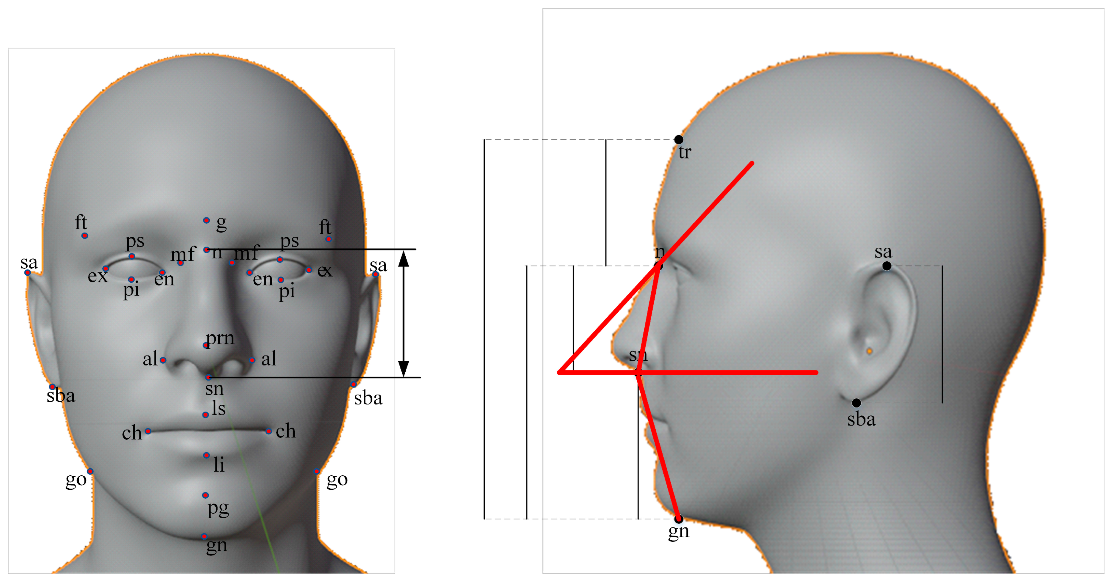
2.1. Facial Landmarks and Used Schemes

Medical landmarks are prominent in 3D facial reconstruction. In computer science, landmarks have different meanings in terms of intended use. The names and definitions of landmarks are presented in studies [29,30]. In nasal reconstruction, a subset of landmarks is used. In computational nasal reconstruction, landmarks can be determined by manual measurement, software, or artificial intelligence image processing. The nasal profile and shape are determined based on the interpolation and analytical methods depending on geometrical parameters and the statistical feature models to reconstruct the nose [31].

Landmarks are the anatomical features of each human face, and their relative positions defined on the soft-tissue surfaces [10] are used for anthropometric reconstruction by both manual and computational methodology (Figure 1). For example, Seshadri et al. [13] implemented the active shape model (denoted as ASM) for locating the landmarks on frontal faces and specified a total of 79 marks which are regarded as optimally and accurately annotated based on facial geometry. Additionally, Zhang, Jie, et al. [13] work on the coarse-to-fine auto-encoder networks (or CFAN) using the landmark’s relative positions for facial detection. Conclusively, the CFAN is superior to the existing DCNN, which is unable to handle fractional stoppage since the points are defined independently from the others [21]. The nasal shape has a geometric relationship with different facial dimensions, such as the distance between several landmark points, depending on some basic shapes with the golden ratio of the face, age, sex, and ethnicity. This study conducts research to evaluate its generalizability, efficiency, and accuracy.

However, for the scope of this research, landmarking is performed manually on images with a locating scheme that has proven efficiency in using denser geometry-based landmarks. There are 17 points used for the nasal reconstruction, and the glabella (denoted as g, Figure 2) is the origin of the coordinate system; thus, from its position of (0, 0, 0), the other points are determined, respectively. In facial surgery or reconstruction, it is necessary to consider the aesthetics of the face after surgery with suitable size and proportions, which ensures that social interaction is not affected. Based on the thickness and histology of the skin on the face, there are 14 cosmetic units, including forehead, right and left cheek, nose, right and left upper eyelid, right and left lower eyelid, right and left ear, upper lip, lower lip, mental area, and neck. Regions 4A and 5B in those affect the nasal shape and reconstruction. Region 4, called the cheek unit, includes a 4A being the medial subunit. Region 5 is the upper lip unit, which is bounded by the nasolabial folds and nasal pillars above, the nasolabial folds on the side, and the inter-lip space below. Sub-region 5B is the lateral subunit. The added points (denoted as int, Figure 3), which locates on the nasal alar, are defined by the intersections of the 3 subunits 2, 4A, and 5B reviewed from [22]. (see Appendix A shows the summary of landmark denotations and definitions)

2.2. How a Dimensional Shape of Nose Is Reconstructed Computationally

Because of the complexity of the nasal surface, it is divided ideally into aesthetic subunits as in [22,23]; hence, its surface is reconstructed sectionally based on the nasal subunit geometry. As the landmarks data are synthesized, interpolation algorithms are implemented; however, only one plane per process is used to generate the other points between chosen landmarks. Thus, for the 3 Cartesian coordinates, x, y, and z, it requires two or more algorithms. Figure 4 shows 2 different samples, the first one with the filled blue dot and the filled red for the second. Accordingly, there are not any blue points that cover the red ones, and vice versa, since the landmark set is distinguished from the others. Based on subunits, our recommended sections’ base splines consist of the mid-line, the alare–pronasale–alare, the mf–int–al, and the al’–int–ac. Sections are covered by the basis splines’ mathematical functions; thus, the surface is the combination of contours generated by points.

3. The Sectional Landmark-Based Reconstruction of Human Nose

Nasal reconstruction is based on two methods of anatomy or morphology to ensure accuracy for reconstruction. The reconstruction is the reproduction of an individual’s nose from facial landmarks. Reconstructing an organ on the face is very difficult, complicated, and time-consuming because its complex shape cannot apply any scientific rule. The reconstruction is a relationship between the virtual facial landmarks and the geometrical parameters of the nose. The image data of the faces are collected with different numbers of groups, such as the age and gender of Vietnamese. In reference to [13], the authors review nasal reconstruction techniques, which are based on plastic surgery to enhance facial shapes, generate organs damaged by accident or disease, and correct deformities… The reconstruction of organs helps patients restore basic functions and aesthetics, which helps improve health utilities.

3.1. The Side Interpolation of Landmarks on the Nasal Bridge (The Mid-Line)

3.1.1. The Polynomial Interpolation of the Nasal Baseline (The Mid-Line)

After the volunteers’ images are processed to erase the background and highlight the nasal baseline (as shown in Figure 5) with the landmarks on it, the shape provokes a polynomial to be applied. Nonetheless, it is impossible to directly use a high-order polynomial, to the naked eye that it does not fit the shape from point g (Glabella–Appendix A) to point k (Kyphion–Appendix A); thus, only the interpolation is implemented except for the g point.

The mathematical model would become a theoretical basis of computational study in complex systems [24]. As shown in Figure 6a, the use of a high-order polynomial causes a significant area error (lateral view–error area bounded by both red solid and dashed lines) that can even be evaluated visually. For Figure 6b, excluding the g-point to perform the interpolation improves over its counterpart; it is obvious that the line is approximately close to the nasal baseline. In this section, the Newton polynomial interpolation is implemented: for a set of k + 1 data points [(x₀, y₀); (x₁, y₂); …; (x_j, y_j); … (x_k, y_k)] without any repeated x_j values, the k-order Newton polynomial P(x) is a linear combination of Newton basis polynomials p_j(x) with their corresponding coefficients w_j.

$$P(x)={\displaystyle \sum _{j=0}^k{w}_j\cdot p_j(x)}$$

(1)

Every polynomial p_j(x) is computed as (2).

$$p_j(x)={\displaystyle \prod _{i=0}^{j-1}(x-x_i)}$$

(2)

where j > 0 and the p₀(x) = 1.

Each coefficient w_j is defined by (3), where every notation [y₀, y₁,…, y_j] denotes the divided differences like as

$$w_j=[y_0,y_1,\dots ,y_j]$$

(3)

In conclusion, the Newton polynomial can be expressed as

$$P(x)=[y_0]+[y_0,y_1]\cdot (x-x_0)+\dots +[y_0,y_1,\dots y_k]\cdot (x-x_0)\cdot (x-x_1)\dots \cdot (x-x_{k-1})$$

(4)

Figure 7 shows the calculation of terms called divided-differences based on the set of k + 1 data points (x_j, f(x_j)) (they can be denoted as (x_j, y_j) or (x_j, f(x_j))) (j is from 0 to k), but the P(x) coefficients only the first term of every stage of computation. The higher order, the more terms are required. For instance, a 2nd Newton polynomial (denoted by the subscript 2 of P₂(x)) is described as (5).

$$P_2(x)=f(x_0)+\frac{f(x_1)-f(x_0)}{(x_1-x_0)}\cdot (x-x_0)+\frac{\frac{f(x_2)-f(x_1)}{(x_2-x_1)}-\frac{f(x_1)-f(x_0)}{(x_1-x_0)}}{(x_2-x_0)}\cdot (x-x_0)\cdot (x-x_1)$$

(5)

3.1.2. The Modified Hyperbolic Function

In this section, the two mf–int–al baselines are interpolated (Figure 8). As the processed images are highlighted, the frontal view of each nose is bounded, and yellow markers ‘X’ locate the landmarks denoted sequentially with mf, int, and al (see Appendix A). The shape of each side boundary (solid red lines) corresponds to the hyperbolic sine; however, this spline should be on another reference system (the red coordinate system) rather than the base system whose origin is the g point (called the g base coordinate). There are two stages for each interpolation of the mf–int–al. The first stage is considered on the frontal view (i.e., the y and z coordinates) with a new reference system whose origin is the mf point (Maxillofrontale–Appendix A, called the mf base coordinate). Interpolating the mf–int–al baseline concerning the g reference system requires three parameters: the angle α between the mf and the g reference system and the center of the O₁ coordinate (Figure 9).

$$T_{mf}^{O_1}\left(\alpha ,d_x,d_y\right)=\left. [\begin{array}{cc}\overline{)\begin{array}{ccc}\cos \left(\alpha \right)& \sin \left(\alpha \right)& 0\\ -\sin \left(\alpha \right)& \cos \left(\alpha \right)& 0\\ 0& 0& 1\end{array}}& \begin{array}{c}{d}_x\\ d_y\\ 0\end{array}\\ \begin{array}{ccccc}0& & 0& & 0\end{array}& 1\end{array}\right]$$

(6)

$$T_{mf}^{O_1}\left(\alpha ,d_x,d_y\right)=\left. [\begin{array}{cc}\overline{)\begin{array}{ccc}\cos \left(\alpha \right)& \sin \left(\alpha \right)& 0\\ -\sin \left(\alpha \right)& \cos \left(\alpha \right)& 0\\ 0& 0& 1\end{array}}& \begin{array}{c}-d_x\cos \left(\alpha \right)-d_y\sin \left(\alpha \right)\\ -d_x\sin \left(\alpha \right)-d_y\cos \left(\alpha \right)\\ 0\end{array}\\ \begin{array}{ccccc}0& & 0& & 0\end{array}& 1\end{array}\right]$$

(7)

To computationally approximate, transposition matrices are used. The $T_{mf}^{O_1}(\alpha ,d_x,d_y)$ expresses the coordinate with the origin of O₁ respecting the system of mf; thus, the $T_{O_1}^{mf}(\alpha ,d_x,d_y)$ helps the mapping and vice versa based on three parameters of α, d_x, and d_y. The algorithm iterates on small step sizes to find the set of $T_{O_1}^{mf}(\alpha ,d_x,d_y)$ parameters that suit the landmarks as close as possible; however, there are such an extreme amount of options for varying the coordinates of the origin O₁ that cost time to find, even if there may be points that are not necessarily needed for the hyperbolic sine function. Hence, the range of search is bounded (see the blue area in Figure 9) based on the two points: int and al positions (related to the mf base coordinate system), and iterations are only stopped when the differences between the generated values and the real points are within the allowed errors (see the whole process in pseudocode of Algorithm 1).

Every iteration requires the calculation of the hyperbolic sine function (8)’s power coefficient β through one set of values (X, Y) respecting the O₁ reference system, and the mf values respecting the O₁ base reference system are recommended. The relation between the power coefficient β and a particular coordinate set is presented in (9).

$$\sinh (x)=\frac{e^{\beta x}-e^{-\beta x}}{2}$$

(8)

$$\beta =\frac{\log \left(y_j+\sqrt{y_j{}^2+1}\right)}{x_j}$$

(9)

where $\left(y_j+\sqrt{y_j{}^2+1}\right)>0$ is the condition for calculating the β.

Algorithm 1: The modified hyperbolic sine (considering points are mapped to the O1 coordinate system). Note: The denotations dx, dy, dx, and dy are only used when considering in two-dimensional space of a set of coordinates

in: The coordinates of 3 landmarks: (mfx, mfy), (intx, inty), and (alx, aly)       The allowed errors: allowed_err,       The step size: step_size.       The angle limits: max_angle, min_angle out: Angle parameter: alpha       The x position: dx       The y position: dy temp: Numerator value: numer            Denominator value: denom            The positional errors: E_int, E_al.            Generated value: gen_int, gen_al            Power coefficient: beta_value 1: dx ← intx; 2: dy ← inty; 3: FOR min_angle ≤ alpha ≤ max_angle 4:     FOR intx ≤ dx ≤ alx 5:            FOR inty ≥ dy ≥ aly 6: $⊳$ Calculating the power coefficient 7:                  numer ← log(mfy + sqrt(pow(mfy, 0.5) + 1)); 8:                  denom ← mfx; 9:                  beta_value ← numer/denom; 10:                   gen_int ← (exp(bet_value * intx) - exp(-                                        beta_value * intx))/2; 11:                   gen_al ← (exp(bet_value * alx) - exp(-                                        beta_value * alx))/2; 12: $⊳$ Calculating the errors 13:                   E_int ← abs(gen_int—inty) 14:                   E_al ← abs(gen_al—aly) 15: $⊳$ Stop the process when conditions are met 16:                    IF E_int ≤ allowed_error && E_al ≤ allowed_error 17:                                      return; 18:                    dy ← dy—step_size; 19:            ENDFOR 20:            dx ← dx + step_size; 21:            dy ← inty; 22:     ENDFOR 23:            alpha ← alpha + step_size; 24:            dx ← intx; 25: ENDFOR

The second stage of this section is to compute the x value for the landmarks; the coordinates of (x, y) of them are considered. For these three points, the Newton 2nd-order polynomial interpolation is recommended since there is not much information between them.

The generated values x, y, and z of the other points are re-mapped corresponding to the g base coordinate and synthesized to form the nasal baselines in Figure 10. In Figure 10 the 3D spatial interpolation results are depicted in Figure 10a, where the mid-line and the mf–int–al interpolation curves have generated the basic shape of the nose according to the desired landmarks. Figure 10b shows the comparison between the interpolation curves according to the modified hyperbolic function and the actual ones of the volunteers. They show that the errors in shape and in position are not large and acceptable.

3.2. The Reconstruction of Nasal Alare–Pronasale–Alare Baseline

3.2.1. The Three-Circle Connection Method

The baseline is formed by three circles that go through every three-point set: the left ac-al-al’, the al’ (left)–prn–al’ (right), and the right ac-al-al’. The computation of each circle is based on three points coordinates as in (10)–(14) by considering P₁, P₂, and P₃ with their corresponding coordinates (x₁, y₁), (x₂, y₂), and (x₃, y₃). The numerical attributes of a circle consisting of the center coordinates x_center, y_center, and the circle radius of R are as follows.

$$x_{center}=\frac{2\cdot A\cdot (y_1-y_3)-2\cdot B\cdot (y_1-y_2)}{4\cdot [(x_1-x_2)\cdot (y_1-y_3)-(x_1-x_3)\cdot (y_1-y_2)]}$$

(10)

$$y_{center}=\frac{2\cdot B\cdot (x_1-x_2)-2\cdot A\cdot (x_1-x_3)}{4\cdot [(x_1-x_2)\cdot (y_1-y_3)-(x_1-x_3)\cdot (y_1-y_2)]}$$

(11)

where:

$$A=(x_1{}^2-x_2{}^2)+(y_1{}^2-y_2{}^2)$$

(12)

$$B=(x_1{}^2-x_3{}^2)+(y_1{}^2-y_3{}^2)$$

(13)

For the computation of radius R, with the values of x_center, and y_center, one set of coordinates is chosen arbitrarily. In (14), P₁ is considered.

$$R=\sqrt{{(x_1-a)}^2+{(y_1-b)}^2}$$

(14)

The attributes are computed by (10)–(14), and the other points on each circle are generated by ranging the value of angle α; for instance, in the circle that goes through the ac-al-al’ set, is between the angle of the ac, and the al’ landmarks. Finally, the baseline is shown in Figure 11.

3.2.2. The Three-Dimensional Alare–Pronasale–Alare Baseline

On the lateral view, the polynomial interpolation is implemented for two four-point sets: the left and right ac-al-al’-prn. As shown in Figure 12 (Left), there is a gap between the two al points; thus, the two sides are distinguished.

3.2.3. The Alar Sidewall Baselines Reconstruction

In Figure 13, the upper curve going through each al’-int-ac set when considering the lateral view is recommended as a part of a circle, which is computed as in (10)–(14). For the top view with only three points, a 2nd order polynomial interpolation is implemented with three unknown coefficients, namely, a₂, a₁ and a₀. Consider three data points (x₀, f(x₀)), (x₁, f(x₁)), and (x₂, f(x₂)); each coefficient is computed (see Appendix B).

3.2.4. The Reconstruction of the Nasal Bottom Section

In Figure 14, the shape of the airflow entrances has sparse landmarks (i.e., only four consisting of the st, cw, la, and lc–Appendix C), which makes the exact shaping of the entrances impossible. Moreover, the ellipse boundary only matches the tilt angle of the entrance and still causes a significant area error (red striped region of Figure 13). Hence, only the surrounding regions are considered, except for the airflow entrances. The reconstruction is conducted along the nasal columella. For the side view, circular curves connecting the al’–st–cw are recommended to form the baselines along the nasal columella by implementing the computations of (10)–(14) (similar to the three-circle connection method–Section 3.2.1). For the frontal view with only 3 points, the 2nd order polynomial as (5) is used. The generated baselines of the columellar are shown in Figure 15.

3.3. The Computational Contouring of Nose

The fully generated three-dimensional nose is the combination of baselines and their contours made by the interpolated line connecting a set of three points on baselines. There are three separated regions to be contoured, namely, the C₁, C₂, and C₃, that are bounded with solid black lines, as shown in Figure 16. The first region of C₁ is contoured with every set of three points coming from the three baselines consisting of the middle line (the mid-line) and the two modified hyperbolic lines on the left and right of it. Considering the ideal nose with high symmetry, from the top view, a parabolic line going through the three points of each set creates a layer. Combining layers of parabolic lines forms a fully contoured region C₁. The interpolation function for each parabolic line is implemented in (5) mentioned previously. For the region of C₂, to remain the shape of the alare–pronasale–alare, the layers are contoured with the same method as their baseline by shifting a d unit step and re-mapping the baseline to fit the continuous solid line of the three baselines: the mid-line and the two hyperbolic shaped lines shown in Figure 17.

Finally, for the region of C₃, with the three baselines of the mid-line and the columellar sidelines, a similar contouring method to the C₁ region is implemented until reaching the endpoints of the columellar sidelines. Combining the points cloud of each region C₁, C₂, and C₃ forms the fully contoured nose, as shown in Figure 18.

4. Evaluations and Discussions

Experiments are conducted with volunteers of different genders based on nasal anthropometric features. The evaluations focus on matching area errors of the generated and the original samples on captured images. There are four samples generated from four volunteers shown in Figure 19. As mentioned in Section 3.3, a contoured nose contains three sections of C₁, C₂, and C₃, which are then continued to be used to evaluate differences in the area between the original and generated noses of each volunteer; however, at this time, each section is separated into subunits (considered as Type in

Table 1. Area errors of samples (Area values are in sq. mm).

View	Section	Type	Sample 1	Sample 2	Sample 3	Sample 4
Frontal	C1	LC1	18.98	15.51	20.98	18.49
Frontal	C1	RC1	25.55	19.39	24.80	26.22
Frontal	C2	AL	−4.50	−3.95	−7.48	−2.09
Frontal	C2	AR	−5.40	−3.53	−4.16	−2.45
Frontal	C3	CL	−99.24	−86.15	−85.35	−75.17
Frontal	C3	CR	−53.39	−73.68	−60.64	−65.23
Lateral	C2	TAL-R	−30.88	−25.54	21.34	−35.48
Lateral	C2	BALR	20.37	15.23	17.34	15.04

Note: The sign of “−” means an uncovered area.

). Errors are summarized in Table 1, and subunits are defined in Appendix D. Table 1 shows the area errors of sub-units within each section, with the highest absolute errors coming from the section of C₃ since this section contains sparse landmarks with less geometry connection between them as mentioned previously in Section 3.3. Those sparse connections of each sample lead to the large, uncovered region below the nose (from the nasal alar to the columellar). For the case of evaluations of both left and right subunits’, area errors are second only to the ones in C₃, which are also caused by the fewer number of points along the mf–int–al baselines. Area errors of sub-units of regions C₁, C₂, and C₃ varied depending on the morphology of the nose as well as ethnicity, sex, and age [32]. The surface of the nose is divided into three regions with different surfaces. The nasal reconstruction depends on the complexity of the nasal regions, which have different errors. In the left and right subunits of section C₁, the range of area errors is from 15.51 to 26.22 mm². In the left and right alare of section C₂, the area error is negative from −7.48 to −2.09 mm² and quite small because the reconstructed surface is within uncovered areas and can be predicted. In the columellar of section C₃ area, the error is negative and larger than that in other sub-regions because landmarks are not labeled to this area. The surface in this region is complex and difficult to describe by mathematical equations for computational discretization. The area errors in the columellar region range from −99.24 to −60.64 mm². In the sub-region of the top of alare, both left and right, the comparison error is both positive and negative depending on the shape of the nose, and the absolute errors are in the range of 21.34 to 35.48 mm². The errors of the bottom of alare both left and right sides are between 15.04 to 20.37 mm². In Table 1, the area errors of sample 1 are the highest due to the complexity of the volunteer’s nose. Based on experiments and measurements, the computational model is quite suitable for the reconstruction of Vietnamese noses with high compatibility. The computational reconstruction as an analytical model would validate with proper experimental results [33,34,35]. Validation is needed to prove the results of a mathematical model in real cases. In this study, computational nasal reconstruction has been developed, and the experimental results have shown that the mathematical model can be used for nasal reconstruction. However, in-depth studies need to confirm the research results as well as be compatible with the morphology of the Vietnamese. In the evaluation between the reconstruction model and reality, the results do not fully reflect the actual value because most of the landmarks on the human face for reconstruction are through frontal and lateral images. Thus, the locations of landmarks, their sizes, and nasal shapes have errors leading to losses in computational reconstruction results.

5. Conclusions

In this paper, a nasal reconstruction model based on facial anthropometrics was researched. However, the study used mainly the anthropometry database of the Vietnamese. Furthermore, several relationships between the dimensional and geometrical shapes of the facial parts were described. However, the study is only preliminary steps based on the experimental regression method. The shape and size of the nose change over time; therefore, the study mainly used data from people under 50 years old, resulting in incomplete reflection of the anthropometric factors to reconstruct the nose by a calculation method. This study presented a mathematical approach directly to facial anthropometrics (e.g., the nasal landmarks) to reconstruct the shape of the nose. Despite the high errors in some regions between the generated and the original nose, we believe that more relations of points from considering a greater number of landmarks can improve the precision of generated baselines and contours.

References

1. Quatrehomme, G.; Gérard, S. Classical non-computer-assisted craniofacial reconstruction. In Computer Graphic Facial Reconstruction; Elsevier: Amsterdam, The Netherlands, 2005; pp. 15–32. [Google Scholar]
2. Clement, J.G.; Marks, M.K. Computer-Graphic Facial Reconstruction; Elsevier: Amsterdam, The Netherlands, 2005. [Google Scholar]
3. Putra, R.U.; Basri, H.; Prakoso, A.T.; Chandra, H.; Ammarullah, M.I.; Akbar, I.; Syahrom, A.; Kamarul, T. Level of Activity Changes Increases the Fatigue Life of the Porous Magnesium Scaffold, as Observed in Dynamic Immersion Tests, over Time. Sustainability 2023, 15, 823. [Google Scholar] [CrossRef]
4. Prakoso, A.T.; Basri, H.; Adanta, D.; Yani, I.; Ammarullah, M.I.; Akbar, I.; Ghazali, F.A.; Syahrom, A.; Kamarul, T. The Effect of Tortuosity on Permeability of Porous Scaffold. Biomedicines 2023, 11, 427. [Google Scholar] [CrossRef] [PubMed]
5. Zhang, Y.; Sim, T.; Tan, C.L.; Sung, E. Anatomy-based face reconstruction for animation using multi-layer deformation. J. Vis. Lang. Comput. 2006, 17, 126–160. [Google Scholar] [CrossRef]
6. Deutsch, C.K.; Shell, A.R.; Francis, R.W.; Bird, B.D. The Farkas System of Craniofacial Anthropometry: Methodology and Normative Databases. In Handbook of Anthropometry: Physical Measures of Human Form in Health and Disease; Springer: Berlin/Heidelberg, Germany, 2012; pp. 561–573. [Google Scholar] [CrossRef]
7. Jayaratne, Y.S.N.; Zwahlen, R.A. Application of Digital Anthropometry for Craniofacial Assessment. Craniomaxillofac. Trauma Reconstr. 2014, 7, 101–107. [Google Scholar] [CrossRef] [PubMed]
8. He, Z.-J.; Jian, X.-C.; Wu, X.-S.; Gao, X.; Zhou, S.-H.; Zhong, X.-H. Anthropometric Measurement and Analysis of the External Nasal Soft Tissue in 119 Young Han Chinese Adults. J. Craniofacial Surg. 2009, 20, 1347–1351. [Google Scholar] [CrossRef]
9. Lazovic, G.D.; Daniel, R.K.; Janosevic, L.B.; Kosanovic, R.M.; Colic, M.M.; Kosins, A.M. Rhinoplasty: The nasal bones–anatomy and analysis. Aesthetic Surg. J. 2015, 35, 255–263. [Google Scholar] [CrossRef]
10. Yang, A.C.Y.; Kretzler, M.; Sudarski, S.; Gulani, V.; Seiberlich, N. Sparse reconstruction techniques in MRI: Methods, applications, and challenges to clinical adoption. Investig. Radiol. 2016, 51, 349. [Google Scholar] [CrossRef] [PubMed]
11. Choi, J.; Medioni, G.; Lin, Y.; Silva, L.; Regina, O.; Pamplona, M.; Faltemier, T.C. 3D face reconstruction using a single or multiple views. In Proceedings of the 2010 20th International Conference on Pattern Recognition, Istanbul, Turkey, 23–26 August 2010; IEEE: New York, NY, USA, 2010; pp. 3959–3962. [Google Scholar]
12. Kemelmacher-Shlizerman, I.; Basri, R. 3D Face Reconstruction from a Single Image Using a Single Reference Face Shape. IEEE Trans. Pattern Anal. Mach. Intell. 2010, 33, 394–405. [Google Scholar] [CrossRef] [PubMed]
13. Vu, N.H.; Trieu, N.M.; Tuan, H.N.A.; Khoa, T.D.; Thinh, N.T. Review: Facial Anthropometric, Landmark Extraction, and Nasal Reconstruction Technology. Appl. Sci. 2022, 12, 9548. [Google Scholar] [CrossRef]
14. Seshadri, K.; Savvides, M. Robust Modified Active Shape Model for Automatic Facial Landmark Annotation of Frontal Faces. In Proceedings of the 2009 IEEE 3rd International Conference on Biometrics: Theory, Applications, and Systems, Washington, DC, USA, 28–30 September 2009; pp. 1–8. [Google Scholar]
15. Zhang, Y.; Prakash, E.C. Face to Face: Anthropometry-Based Interactive Face Shape Modeling Using Model Priors. Int. J. Comput. Games Technol. 2009, 2009, 1–15. [Google Scholar] [CrossRef]
16. Egelhoff, K.; Idzi, P.; Bargiel, J.; Wyszyńska-Pawelec, G.; Zapała, J.; Gontarz, M. Implementation of Cone Beam Computed Tomography, Digital Sculpting and Three-Dimensional Printing in Facial Epithesis—A Technical Note. Appl. Sci. 2022, 12, 11974. [Google Scholar] [CrossRef]
17. Mamsen, F.P.W.; Kiilerich, C.H.; Hesselfeldt-Nielsen, J.; Saltvig, I.; Remvig, C.L.-N.; Trøstrup, H.; Schmidt, V.-J. Risk Stratification of Local Flaps and Skin Grafting in Skin Cancer-Related Facial Reconstruction: A Retrospective Single-Center Study of 607 Patients. J. Pers. Med. 2022, 12, 2067. [Google Scholar] [CrossRef] [PubMed]
18. Saraswathula, A.; Porras, J.L.; Mukherjee, D.; Rowan, N.R. Quality of Life Considerations in Endoscopic Endonasal Management of Anterior Cranial Base Tumors. Cancers 2023, 15, 195. [Google Scholar] [CrossRef]
19. Huang, C.-C.; Wu, P.-W.; Huang, C.-C.; Chang, P.-H.; Fu, C.-H.; Lee, T.-J. Identifying Residual Psychological Symptoms after Nasal Reconstruction Surgery in Patients with Empty Nose Syndrome. J. Clin. Med. 2023, 12, 2635. [Google Scholar] [CrossRef] [PubMed]
20. Larimi, M.; Babamiri, A.; Biglarian, M.; Ramiar, A.; Tabe, R.; Inthavong, K.; Farnoud, A. Numerical and Experimental Analysis of Drug Inhalation in Realistic Human Upper Airway Model. Pharmaceuticals 2023, 16, 406. [Google Scholar] [CrossRef] [PubMed]
21. Li, H.; Wang, J.; Song, T. 3D Printing Technique Assisted Autologous Costal Cartilage Augmentation Rhinoplasty for Patients with Radix Augmentation Needs and Nasal Deformity after Cleft Lip Repair. J. Clin. Med. 2022, 11, 7439. [Google Scholar] [CrossRef]
22. Martín-Jiménez, M.; Pérez-García, A. Neuroanatomical Study and Three-Dimensional Cranial Reconstruction of the Brazilian Albian Pleurodiran Turtle Euraxemys essweini. Diversity 2023, 15, 374. [Google Scholar] [CrossRef]
23. Guevara, C.; Matouk, M. In-office 3D printed guide for rhinoplasty. Int. J. Oral Maxillofac. Surg. 2021, 50, 1563–1565. [Google Scholar] [CrossRef]
24. Tauviqirrahman, M.; Jamari, J.; Susilowati, S.; Pujiastuti, C.; Setiyana, B.; Pasaribu, A.H.; Ammarullah, M.I. Performance Comparison of Newtonian and Non-Newtonian Fluid on a Heterogeneous Slip/No-Slip Journal Bearing System Based on CFD-FSI Method. Fluids 2022, 7, 225. [Google Scholar] [CrossRef]
25. Gordon, A.R.; Schreiber, J.E.; Patel, A.; Tepper, O.M. 3D Printed Surgical Guides Applied in Rhinoplasty to Help Obtain Ideal Nasal Profile. Aesthetic Plast. Surg. 2021, 45, 2852–2859. [Google Scholar] [CrossRef]
26. Paysan, P.; Knothe, R.; Amberg, B.; Romdhani, S.; Vetter, T. A 3D Face Model for Pose and Illumination Invariant Face Recognition. In Proceedings of the IEEE International Conference on Advanced Video and Signal Based Surveillance, Genova, Italy, 2–4 September 2009; pp. 296–301. [Google Scholar]
27. Ammarullah, M.I.; Hartono, R.; Supriyono, T.; Santoso, G.; Sugiharto, S.; Permana, M.S. Polycrystalline Diamond as a Potential Material for the Hard-on-Hard Bearing of Total Hip Prosthesis: Von Mises Stress Analysis. Biomedicines 2023, 11, 951. [Google Scholar] [CrossRef] [PubMed]
28. Jamari, J.; Ammarullah, M.I.; Santoso, G.; Sugiharto, S.; Supriyono, T.; Permana, M.S.; Winarni, T.I.; van der Heide, E. Adopted walking condition for computational simulation approach on bearing of hip joint prosthesis: Review over the past 30 years. Heliyon 2022, 8, e12050. [Google Scholar] [CrossRef] [PubMed]
29. Tauviqirrahman, M.; Ammarullah, M.I.; Jamari, J.; Saputra, E.; Winarni, T.I.; Kurniawan, F.D.; Shiddiq, S.A.; van der Heide, E. Analysis of contact pressure in a 3D model of dual-mobility hip joint prosthesis under a gait cycle. Sci. Rep. 2023, 13, 3564. [Google Scholar] [CrossRef] [PubMed]
30. Tuan, H.N.A.; Hai, N.D.X.; Thinh, N.T. Shape prediction of nasal bones by digital 2D-photogrammetry of the nose based on convolution and back-propagation neural network. Comput. Math. Methods Med. 2022, 2022, 5938493. [Google Scholar] [CrossRef]
31. Trieu, N.M.; Thinh, N.T. The Anthropometric Measurement of Nasal Landmark Locations by Digital 2D Photogrammetry Using the Convolutional Neural Network. Diagnostics 2023, 13, 891. [Google Scholar] [CrossRef]
32. Diac, M.M.; Earar, K.; Damian, S.I.; Knieling, A.; Iov, T.; Shrimpton, S.; Castaneyra-Ruiz, M.; Wilkinson, C.; Iliescu, D.B. Facial Reconstruction: Anthropometric Studies Regarding the Morphology of the Nose for Romanian Adult Population I: Nose Width. Appl. Sci. 2020, 10, 6479. [Google Scholar] [CrossRef]
33. Salaha, Z.F.M.; Ammarullah, M.I.; Abdullah, N.N.A.A.; Aziz, A.U.A.; Gan, H.-S.; Abdullah, A.H.; Kadir, M.R.A.; Ramlee, M.H. Biomechanical Effects of the Porous Structure of Gyroid and Voronoi Hip Implants: A Finite Element Analysis Using an Experimentally Validated Model. Materials 2023, 16, 3298. [Google Scholar] [CrossRef]
34. Hsu, W.-C.; Chou, L.-W.; Chiu, H.-Y.; Hsieh, C.-W.; Hu, W.-P. A Study on the Effects of Lateral-Wedge Insoles on Plantar-Pressure Pattern for Medial Knee Osteoarthritis Using the Wearable Sensing Insole. Sensors 2023, 23, 84. [Google Scholar] [CrossRef]
35. Lamura, M.D.P.; Hidayat, T.; Ammarullah, M.I.; Bayuseno, A.P.; Jamari, J. Study of contact mechanics between two brass solids in various diameter ratios and friction coefficient. Proc. Inst. Mech. Eng. Part J J. Eng. Tribol. 2023, 14657503221144810. [Google Scholar] [CrossRef]
36. Zhang, J.; Shan, S.; Kan, M.; Chen, X. Coarse-to-Fine Auto-Encoder Networks (cfan) for Real-Time Face Alignment. In Proceedings of the Computer Vision–ECCV 2014: 13th European Conference, Zurich, Switzerland, 6–12 September 2014; Proceedings, Part II 13. Springer International Publishing: New York, NY, USA, 2014; pp. 1–16. [Google Scholar]
37. Fattahi, T.T. An overview of facial aesthetic units. J. Oral Maxillofac. Surg. 2003, 61, 1207–1211. [Google Scholar] [CrossRef]
38. Based, A.D.; Ilankovan, V.; Ethunandan, M.; Seah, T.E. Local Flaps in Facial Reconstruction; Springer: Berlin/Heidelberg, Germany, 2007. [Google Scholar]
Figure 1. Basic facial landmarks and their anthropometric characteristics located on soft tissues.
Mathematics 11 02456 g001
Figure 2. Depiction of landmarks used in research: (a) Frontal view; (b) Lateral view.
Mathematics 11 02456 g002
Figure 3. The facial aesthetic units.
Mathematics 11 02456 g003
Figure 4. Synthesized 3 coordinates data of 2 different landmark-set from 2 volunteers: (a) Perspective view; (b) Frontal view; and (c) Lateral view (blue for the first and red for the second volunteers).
Mathematics 11 02456 g004
Figure 5. Volunteers and their corresponding processed images of the nasal bridge (on the left of each image).
Mathematics 11 02456 g005
Figure 6. Interpolation of the nasal bridge of a particular volunteer, (a): The high-order polynomial with dashed lines (both red and blue color) and the nasal baseline with a solid red line; (b): Interpolation except for g point (solid orange line).
Mathematics 11 02456 g006
Figure 7. The calculation of divided differences in Newton polynomial interpolation, (a) The tabular calculation method; (b): Pseudo code for computer program.
Mathematics 11 02456 g007
Figure 8. The volunteers and their processed images of nasal frontal view (to the left of each portrait).
Mathematics 11 02456 g008
Figure 9. The coordinate systems depict the algorithm (at a particular instance). Note: The y and z values become X and Y correspondingly when considering them in two dimensions; thus, an applied transposition matrix contains a rotation about the Z axis.
Mathematics 11 02456 g009
Figure 10. The interpolated results of the mid-line and the mfintal: (a) The three-dimensional model; (b) The shape comparison.
Mathematics 11 02456 g010
Figure 11. The connected alare–pronasale–alare baseline.
Mathematics 11 02456 g011
Figure 12. The three-dimensional model of the alare–pronasale–alare baseline. (left): Isometric view; (right): Lateral view.
Mathematics 11 02456 g012
Figure 13. The three-dimensional model of the nose with generated baselines, (a): Isometric view, (b): Frontal view, and (c): Side view.
Mathematics 11 02456 g013
Figure 14. The bottom view of nose and its landmarks.
Mathematics 11 02456 g014
Figure 15. The three-dimensional baselines of the nose, (a): Frontal view, and (b): Side view.
Mathematics 11 02456 g015
Figure 16. The three regions of contouring C1, C2, and C3.
Mathematics 11 02456 g016
Figure 17. The contouring process of the C2 region.
Mathematics 11 02456 g017
Figure 18. The fully contoured three-dimensional nose shape based on landmarks: (a) Frontal view, (b) Lateral view.
Mathematics 11 02456 g018
Figure 19. Nose samples from volunteers used in evaluation: (A) Sample 1; (B) Sample 2; (C) Sample 3, and (D) Sample 4.
Mathematics 11 02456 g019