Article

Swarm Robots Search for Multiple Targets Based on Historical Optimal Weighting Grey Wolf Optimization

Software College, Northeastern University, Shenyang 110169, China
*
Author to whom correspondence should be addressed.
Mathematics 2023, 11(12), 2630; https://doi.org/10.3390/math11122630
Submission received: 28 April 2023 / Revised: 29 May 2023 / Accepted: 7 June 2023 / Published: 8 June 2023

Abstract

:
This study investigates the problem of swarm robots searching for multiple targets in an unknown environment. We propose the Historical Optimal Weighting Grey Wolf Optimization (HOWGWO) algorithm based on an improved grouping strategy. In the HOWGWO algorithm, we gather and update every individual grey wolf’s historical optimal position and rank grey wolves based on the merit of their historical optimal position. The position of the prey is dynamically estimated by the leader wolf, and all grey wolves move towards the prey’s estimated position. To solve the multi-target problem of swarm robots search, we integrate the HOWGWO algorithm with an improved grouping strategy and divide the algorithm into two stages: the random walk stage and the dynamic grouping stage. During the random walk stage, grey wolves move randomly and update their historical optimal positions. During the dynamic grouping stage, the HOWGWO algorithm generates search auxiliary points (SAPs) by adopting an improved grouping strategy based on individual grey wolves’ historical optimal positions. These SAPs are then utilized for grouping grey wolves to search for different prey. The SAPs are re-generated using the optimum historical positions of every single grey wolf after positions have been updated, rather than just those belonging to a specific group. The effectiveness of the proposed HOWGWO algorithm is extensively assessed in 30 dimensions using the CEC 2017 test suite, which simulates unimodal, multimodal, hybrid, and composition problems. Then, the obtained results are compared with competitors, including GWO, PSO and EGWO, and the results are statistically analyzed through Friedman’s test. Ultimately, simulations are performed to simulate the problem of searching multiple targets by swarm robots in a real environment. The experimental results and statistical analysis confirm that the proposed HOWGWO algorithm has a fast convergence speed and solution quality for solving global optimization problems and swarm robots searching multiple targets problems.

1. Introduction

Swarm intelligence represents an interdisciplinary field in AI technology. In this field, swarm individuals detect and recognize targets, independently decide about the environment, interact with other swarm information, and evolve in a manner that demonstrates self-organization, collaboration, stability, flexibility, and adaptability to the environment [1]. A swarm robot network consists of interconnected robotic devices with relatively simple functions that collaborate in clusters to accomplish tasks [2,3]. Swarm robots, compared to individual robots, can explore unknown environments collaboratively through parallel processing, task distributivity, information redundancy, flexibility, and fault tolerance capabilities. These capabilities enable efficient and reliable task completion in complex environments [4,5]. Swarm robot technology can be widely used in uncharted space exploration (such as planet exploration) [6,7,8], environmental monitoring [9,10,11], post-disaster human search and rescue [12,13,14], target roundup [15], hazard detection [16], and other tasks, and it has a wide range of applications in military, industrial, and civil fields [17,18].
Swarm robotics systems have a key role in target search, which is crucial in various domains, such as search and rescue, natural resource exploration, detecting signal sources, and locating enemies [19]. Many researchers have utilized swarm intelligence strategies to develop effective search capabilities in swarm robotics systems. Ref. [20] proposed a hybrid evolutionary algorithm that combines an evolutionary local search (ELS) with a heuristic based on the Randomized Extended Clarke and Wright Algorithm (RECWA) to create feasible solutions. Tan et al. [21] proposed a robot target tracking algorithm based on a group search strategy, which can self-adaptively divide populations according to environmental characteristics to solve problems related to obstacle avoidance in complex search environments. In [22], a particle swarm algorithm based on a clustering method was proposed for solving the problem of searching for multi-robot dynamic targets. Ref. [23] investigated the issue of searching for multiple targets by swarm robots in unknown environments and presented a distributed algorithm called A-RPSO (Adaptive Robotic PSO) based on particle swarm optimization (PSO). This algorithm considers obstacle avoidance and possesses a mechanism to avoid local optima, which gives it good performance in large-scale environments with few robots. However, it is only applicable to scenarios where a single target is being searched for. Tang et al. in [24] combined fruit fly optimization with particle swarm optimization to address issues of population diversity and local optima avoidance in target search by swarm robots. In [25], a Lévy-walk and firefly-based algorithm (LFA) was proposed, where the former focuses on exploration, and the latter emphasizes exploitation. Ref. [26] discussed a hybrid optimization approach combining an evolutionary method and a gradient-based method using an efficient weighting function to obtain a deterministic solution for a real-world problem. Ref. [27] proposed an improved Moth Flame Optimization (MFOSFR) algorithm that addresses the local optimum entrapment and premature convergence common in MFO algorithms by introducing an effective stagnation, finding, and replacing (SFR) strategy to maintain population diversity. Ref. [28] introduced a grouping strategy and random walk phase into the Constriction Factors Particle Swarm Optimization (CFPSO) and considered obstacle avoidance, mutual avoidance of robots, and the influence range of the target, which are more realistic. However, this method relies on the number of random wandering phases to adjust the number of groups using the advantages of group robots, and it cannot dynamically change the number of groups.
This paper presents a novel approach to optimizing the updating mechanism of Searching Auxiliary Points (SAPs) within the grouping strategy [28] using the Grey Wolf Optimization (GWO) [29] algorithm, which is a swarm intelligence algorithm inspired by the hunting habits of grey wolves. Our method combines the SAP optimization with the improved Grey Wolf Optimization algorithm, that utilizes a historical optimal position updating strategy to enhance information retrieval from the robot’s position history. We introduce a novel algorithm termed Historical Optimal Weighting Grey Wolf Optimization (HOWGWO), which integrates the historical positional information prior to optimizing the weight function in the grouping strategy. Overall, the following are the primary contributions of this work.
(a) We present the HOWGWO algorithm based on an enhanced grouping strategy, which improves the performance and enriches the diversity of canonical GWO;
(b) We introduce a historical optimal weighting strategy to rank the grey wolves according to the historical optimal positions and guide the update of all grey wolf positions to improve the search performance;
(c) We introduce a grouping strategy to divide the populations into groups in order to increase diversity.
The performance of the proposed HOWGWO algorithm is assessed with the CEC 2017 test functions in 30 dimensions. Then, the HOWGWO algorithm is compared with the grey wolf optimization algorithm (GWO) [29], the particle swarm optimization algorithm (PSO) [30], and the enhanced grey wolf optimization algorithm (EGWO) [31]. Furthermore, the results obtained using the proposed algorithms are statistically analyzed using the Wilcoxson test. Finally, an application problem in a simulation scenario is considered, and the HOWGWO algorithm is compared with the grouping-based CFPSO algorithm. Statistical results show that the proposed HOWGWO algorithm was superior to the contender algorithms.
The remainder of this paper is structured as follows. In Section 2, we introduce the problem that is the focus of our investigation. Then, Section 3 offers a detailed presentation of the historical optimal weight and grouping strategy, which serves as the basis for our proposed solution. In Section 4, we conduct a Wilcoxson rank sum test and comparative experiments and provide the convergence curve analysis. In Section 5, we present our simulations, comparisons, and a discussion of our results, and we provide an overview of the evaluation criteria used. Finally, Section 6 concludes the paper by summarizing our findings and discussing their implications, as well as potential avenues for future research.

2. Problem Statement

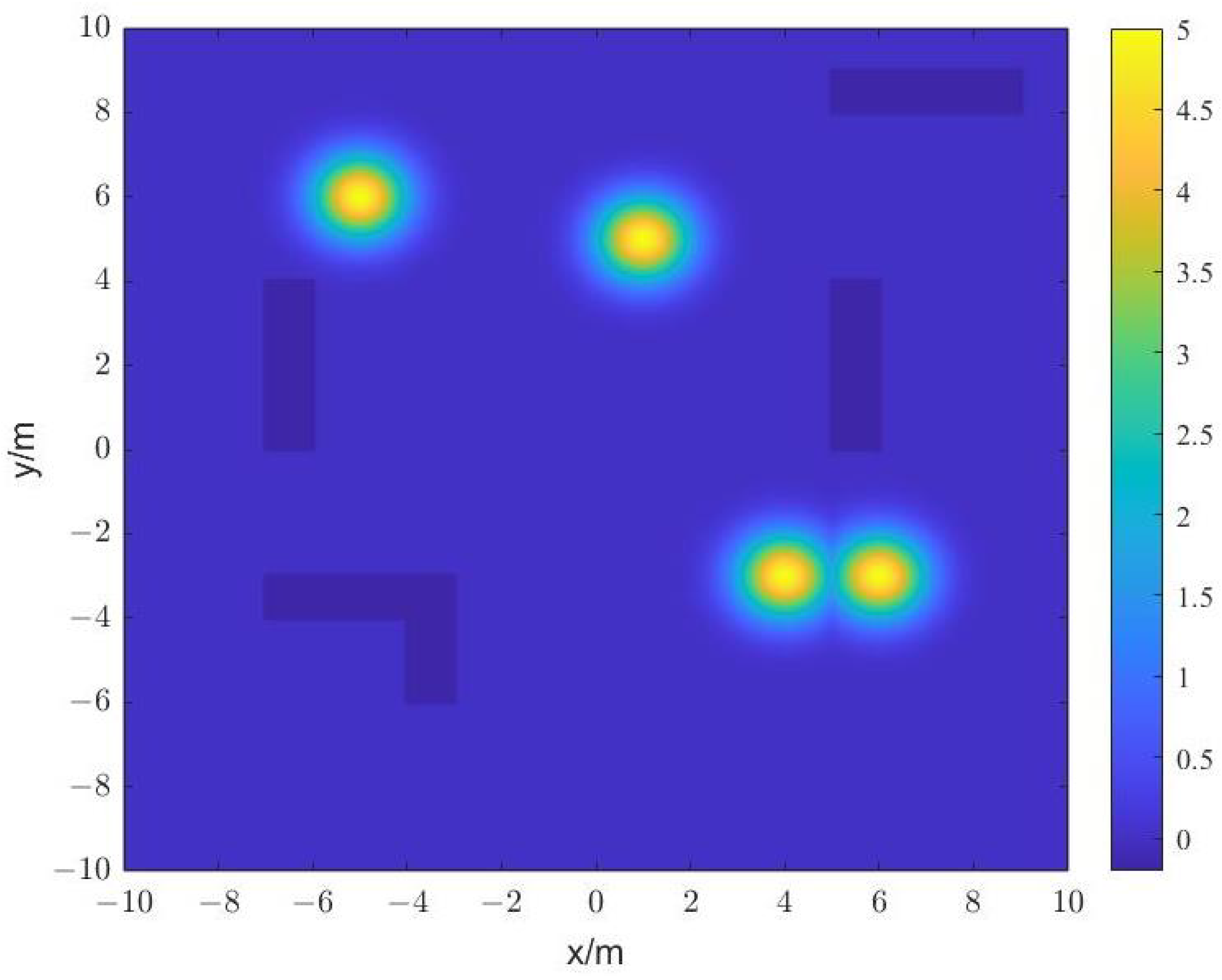
In this paper, we investigate a rectangular search area of dimensions L x × L y containing obstacles represented by polygons, as illustrated in Figure 1. It is assumed that all targets are randomly dispersed throughout the search area and emit light or radiation as a signal that decreases gradually with increasing distance from the target, rendering it invisible beyond a certain range. The signal strength encompasses a range of 0 to 5, as shown in the chromatic scale in Figure 2 (the signal type is decided by the actual situation, and the value represents the relative size).
The robot is designed to be an omnidirectional mobile robot that can move in any direction without turning. The robots are required to independently plan their path toward their pre-programmed destination while avoiding obstacles and collisions with other robots. Each of the robots is equipped with sensors to detect the signal strength of the target and share the collected information through the network module. During each search iteration, the robot detects the signal strength of its current location and shares it with other robots when it moves to a new location and stops moving.

3. Algorithm Statement

3.1. Grey Wolf Optimization Based on Historical Optimal Weight Estimation

The Grey Wolf Optimization is based on the hierarchical social structure and hunting behavior of grey wolves, where the top-ranking α -wolf makes decisions for the population’s hunting activities, and the intermediate-level β -wolf and δ -wolf assist with decision-making by presenting the second- and third-best solutions found. The grey wolf population’s hunting behavior is guided cooperatively by the first three ranks of wolves:
D α = C 1 · X α X , D β = C 2 · X β X , D δ = C 3 · X δ X
X 1 = X α A 1 · D α , X 2 = X β A 2 · D β , X 3 = X δ A 3 · D δ
X t + 1 = X 1 + X 2 + X 3 3
where t indicates the current iteration, A 1 , 2 , 3 are C 1 , 2 , 3 coefficient vectors, X α , β , δ is the position vector of the prey, and X 1 , 2 , 3 indicates the position vector of a grey wolf. The vectors A 1 , 2 , 3 and C 1 , 2 , 3 are calculated as follows:
A 1 , 2 , 3 = 2 a · r 1 a
C 1 , 2 , 3 = 2 · r 2
where components of a linearly decrease from 2 to 0 over the course of iterations and r 1 , r 2 are random vectors in [ 0 , 1 ] .
The proposed approach differs from the original grey wolf optimization by incorporating a dynamic estimation process to determine the prey’s location based on its weight [31]:
X p = ω α · X α t + ω β · X β t + ω δ · X δ t + ϵ t
where X p indicates the estimated position of the prey.
To leverage the past position information of grey wolf individuals, we store the historical optimal positions of all grey wolf individuals at the t-th iteration using P i t . We then update P α , β , δ t , which replaces X α , β , δ t , in the following way:
P i ( t ) = P i ( t 1 ) , f X i ( t ) f P i ( t 1 ) X i ( t ) , f X i ( t ) > f P i ( t 1 ) .
Here, X i t represents the position vector of grey wolf individual i at the t-th iteration, and it is a feasible solution to the solved problem within the range [ X m a x , X m a x ] . f X i t denotes the fitness value of the feasible solution; in this paper, it represents the signal intensity magnitude of the target detected by the swarm robot at a specific position. The variable t spans over iterations 1 m . Thus, Equation (6) can be reformulated as:
X p = ω α · P α t + ω β · P β t + ω δ · P δ t + ϵ t
where ω α , β , δ represents the weight of the grey wolves in estimating the prey’s location, and the term ϵ t denotes the random tolerance. It conforms to the normal distribution N ( 0 , σ ( t ) ) where σ t > σ ( t + 1 ) and σ t = 1 t / G for G being the maximum number of iterations. The weight ω reflects the grey wolf’s dominance in position guidance.
The weight relationship between different levels of grey wolves is determined by the following inequalities:
1 ω α ω β ω δ 0
ω α + ω β + ω δ = 1 ,
and weight values are updated based on the fitness functions by using the following equations. More precisely, if the fitness function f ( · ) is maximized,
ω α = f P α f P α + f P β + f P δ
ω β = f P β f P α + f P β + f P δ
ω δ = f P δ f P α + f P β + f P δ
otherwise,
ω α = 0.5 * 1 f i t P α f i t P α + f i t P β + f i t P δ
ω β = 0.5 * 1 f i t P β f i t P α + f i t P β + f i t P δ
ω δ = 0.5 * 1 f i t P δ f i t P α + f i t P β + f i t P δ
where f ( · ) represents the fitness function.
Each wolf in the population is directed by the leader towards the estimated position of the prey, which is denoted by X p . The estimated position is calculated using the equation:
X i t + 1 = X p t r · X p t P i t
where the i-th grey wolf’s historical optimal position vector at the t-th iteration is denoted by P i , and r is a uniformly distributed random number on the interval [ 2 , 2 ] . If r > 1 , the proposed algorithm will explore new local optima; otherwise, it will continue to exploit a local optimal solution around the estimated location of the prey. Thus, the population behavior of grey wolves can be characterized in terms of r > 1 indicating prey hunting and r < 1 indicating prey attack. It is worth noting that the variation range of random number r does not decrease linearly from 2 to 0 throughout the sequence of iterations. Otherwise, in the latter half of the iterations, the algorithm will continuously exploit a local optimal solution because r 2 * 1 t / G if t > G / 2 . Moreover, the fundamental difference is that the base χ p j t in the proposed operation is a dynamically integrated point rather than an existing solution in the current population.
If an individual grey wolf exceeds the search boundary limit, the algorithm will rectify this by causing it to move spontaneously towards the boundary crossed. This movement is determined by Equation (18), which characterizes the random walking behavior of grey wolves during the hunting process
X i ( t + 1 ) = X i ( t ) + u · U X i ( t ) , i f X i ( t + 1 ) > U X i ( t ) + u · L X i ( t ) , i f X i ( t + 1 ) < L
where U and L are boundary vectors, and the random number u is uniformly distributed from −2 to 2. This arbitrary movement can characterize, to some extent, the random walking behavior of the wolf in the process of hunting for prey.

3.2. Random Walk Stage—First Stage

The initial positions of the robots are randomly generated throughout the search area, with the exception of areas that were occupied by obstacles, and then their positions are updated by
X i t + 1 = X i t + U · 1 + 2 r · t
where t is the number of iterations, r is a random value in [0, 1], X i ( t ) represents the position of the i-th grey wolf individual at the tth time, and U is the boundary vector.
In this stage, the robots move randomly to explore the search area as much as possible for the purpose of gathering information. This collected information is used in the second stage of decision-making. It is of the utmost importance, in this stage, that the entire search area is explored in the shortest possible time. The number of iterations in the initial stage is calculated as η · N i , where η is the percentage factor, and N i is the total number of iterations across both stages.

3.3. Dynamic Grouping Stage—Second Stage

The dynamic grouping strategy divides a large population into multiple tiny subgroups to hunt for different prey, while ensuring some information exchange between every subgroup. This information exchange is reflected in the regrouping after each position update, i.e., dynamic grouping, while each group searches for different targets separately. Combining the grouping strategy with the historical optimal weighted grey wolf optimization algorithm not only exploits but also extends the optimization algorithm’s powerful optimizing ability, allowing the combined optimization algorithm to search multiple target points simultaneously.

3.3.1. Searching Auxiliary Points (SAPs) Generation

This paper employs the searching auxiliary points (SAPs) generation strategy proposed in [28]. The term SAPs refers to points in the target area that demonstrate a high signal strength. These positions guide the robots to the precise locations of the targets. The closer SAPs are to the center of the target, the stronger the signal strength becomes, which makes them exceptionally significant. The second stage involves the grouping of robots based on the SAPs, with each one being assigned a group. Typically, the number of groups is equal to the number of SAPs and target points.
The identification of suitable historical optimal positions H i for generating SAPs is crucial for the performance of the algorithm. However, not all historical optimal positions are equally effective as reference points for generation of SAPs. This is because, in most cases, regions far from the target display weak signal strengths. Therefore, historical optimal positions generated in those areas do not provide relevant information for determination of SAPs. To solve this issue, we define a threshold value f t h to filter out these positions. Only the historical optimal positions with high signal strength, which individual robots retain, are considered as candidate positions C p for generation of SAPs. We then sort the candidate positions C p in descending order of signal strength and select the position with the greatest signal strength S p 1 as the SAP. The remaining candidate positions C p are evaluated based on:
S p M s m a k e d s p , C p > l d
where S p denotes any known SAP, M s is the set containing all known SAPs, C p is the candidate position to be judged, and d s p , C p is the distance between S p and C p . If the distance between a candidate location and all known SAPs is larger than l d , then it can be considered as SAP, otherwise, the following judgment should be further executed:
p r M r m a k e f p r < f ( S p ) , f p r < f ( C p ) w h e r e d S p , C p l d
where f ( S p ) denotes the fitness of the SAP, and f ( C p ) is the fitness of the candidate position. Moreover, M r is the set of uniformly distributed points on the line between S p and C p , and p r is any reference position in M r . Equation (21) guarantees that each target point is followed by at least one SAP.
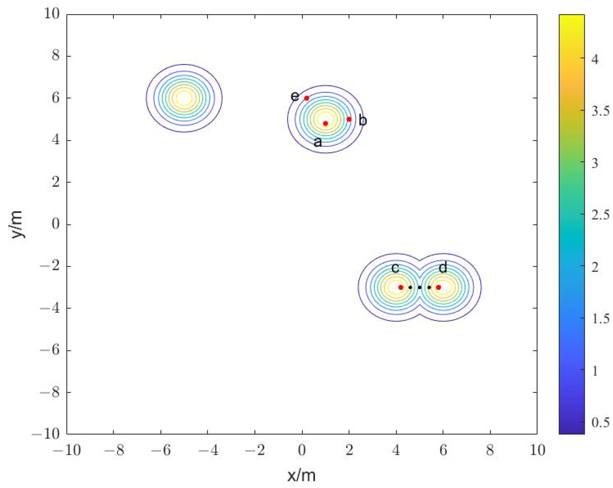
The following paragraph provides an overview of the process employed to select SAPs using a specific algorithm. Figure 3 depicts five candidate positions, represented by a, b, c, d, and e, ranked by signal strength as f ( a ) > f ( c ) > f ( d ) > f ( b ) > f ( e ) , and highlights SAPs a and c based on the applied Equation (20). However, position d, despite not satisfying Equation (20), is proximate to a distinct target compared to the one approached by c and should also be identified as a SAP. In this case, reference positions between position c and d are illustrated by black dots, and their signal strength is compared to f ( S p ) and f ( C p ) . Equation (21) is used to determine whether position d approaches a different target from the known SAPs. If Equation (21) is satisfied, position d is annotated as a new SAP. Positions b and e are not considered as SAPs because they fail to satisfy either Equation (20) or (21).

3.3.2. Dynamic Grouping and Searching

After examining all possible candidate points, we can group the robots based on the generated SAPs. The robots will adhere to the "proximity" principle when being grouped. This principle states that each robot should join the group containing the SAP closest to their current position. There should be an equal number of groups of robots and SAPs available. Robot i will be assigned to the m-th group according to:
S k M s m a k e d r i , s k = min d r i , s 1 , d r i , s 2 , , d r i , s k
where S k is any SAP, r i is the position of robot i, d r i , s k represents the distance between robot i and the m-th SAP, and M s is the set of SAPs. After robots are grouped, any interaction between them can only occur within the group, and each group’s robot’s position is updated via Equations (8) and (17).
Compared with the dynamic grouping strategy in [28], the improved dynamic grouping strategy has superior adaptability in this study. The grouping strategy ought to be able to adjust not only in structure but also in the number of groups, which is not satisfied by the original grouping strategy. In the second stage, once all search agents’ locations have been updated, the previous search auxiliary points would no longer be used, and the algorithm will then regenerate new search auxiliary points using Equations (20) and (21) and regroup all search agents using Equation (22). This increases the likelihood of finding all targets by increasing the consistency among the number of groupings and the actual number of targets.
The signal strength in the majority of the simulated experimental regions exhibits values close to zero. Thus, Equation (7), which updates the historical optimal positions of each robot, has been adjusted as follows:
P i ( t ) = P i ( t 1 ) , f X i ( t ) < f P i ( t 1 ) X i ( t ) , f X i ( t ) f P i ( t 1 ) .
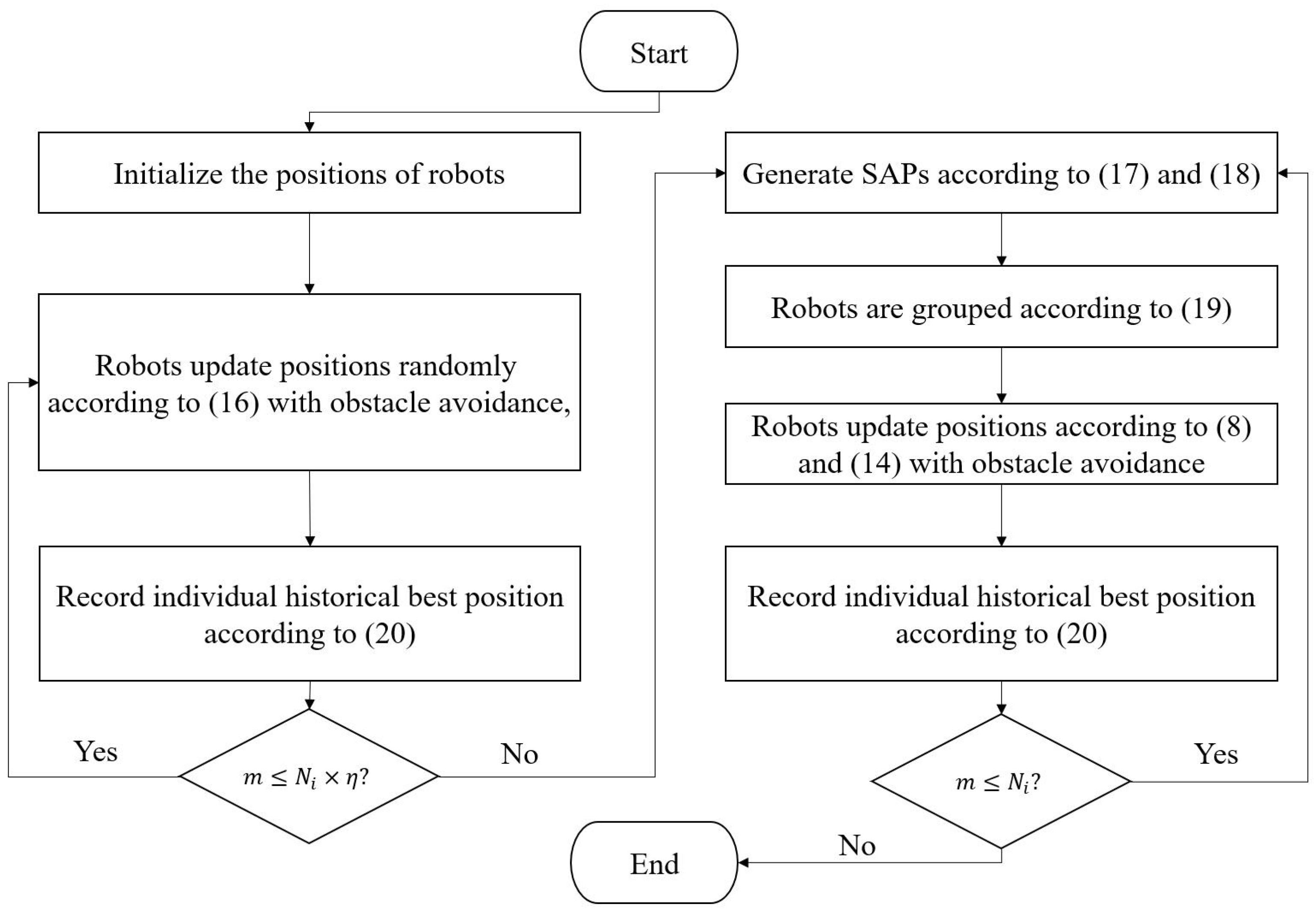
At the end of each iteration, the historical optimal positions of each robot are updated using Equation (23). Subsequently, based on Equations (20) and (21), the positions of SAPs are regenerated. Using the new SAPs, the robots are regrouped before moving on to the next search iteration. The objective of this step is to ensure that the SAPs are positioned near each designated target during the dynamic grouping stage. Our approach continually updates the number of SAPs during the robots’ search process as opposed to the fixed approach in [25]. This is to prevent situations where the number of targets exceeds the set number of SAPs, which provides the robots with a search strategy that can locate all targets. Finally, each group of robots is assigned to a different target, and the entire environment is searched for all targets. The flowchart of the algorithm is shown in Figure 4. The procedure is described by Algorithm 1.
Algorithm 1 Position update strategies in HOWGWO
1:
Start;
2:
Initialize a grey wolf population(robots), Iteration times: N i , Percentage factor of iteration: η ;
3:
Evaluate each individual using the fitness function f ( x ) and initialize individual robot’s historical optimal position, denoted as P t ;
4:
while  t < N i   do
5:
    if  t < N i · η  then
6:
        Update the position of wolf (robot) by Equation (19);
7:
        Update the historical optimal position of wolf by Equation (23);
8:
    else
9:
        Generate ‘Searching Auxiliary Points(SAPs)’, donated as S p , by Equations (20) and (21);
10:
       Group the grey wolf (robot) by Equation (22);
11:
       Update the position of grey wolf (robot) in each group by Equations (8), (11), (12), (13) and (17);
12:
       Update the historical optimal position of grey wolf (robot) by Equation (23);
13:
    end if
14:
end while
15:
Output the locations of targets;
16:
End.

3.4. Obstacle Avoidance Strategy

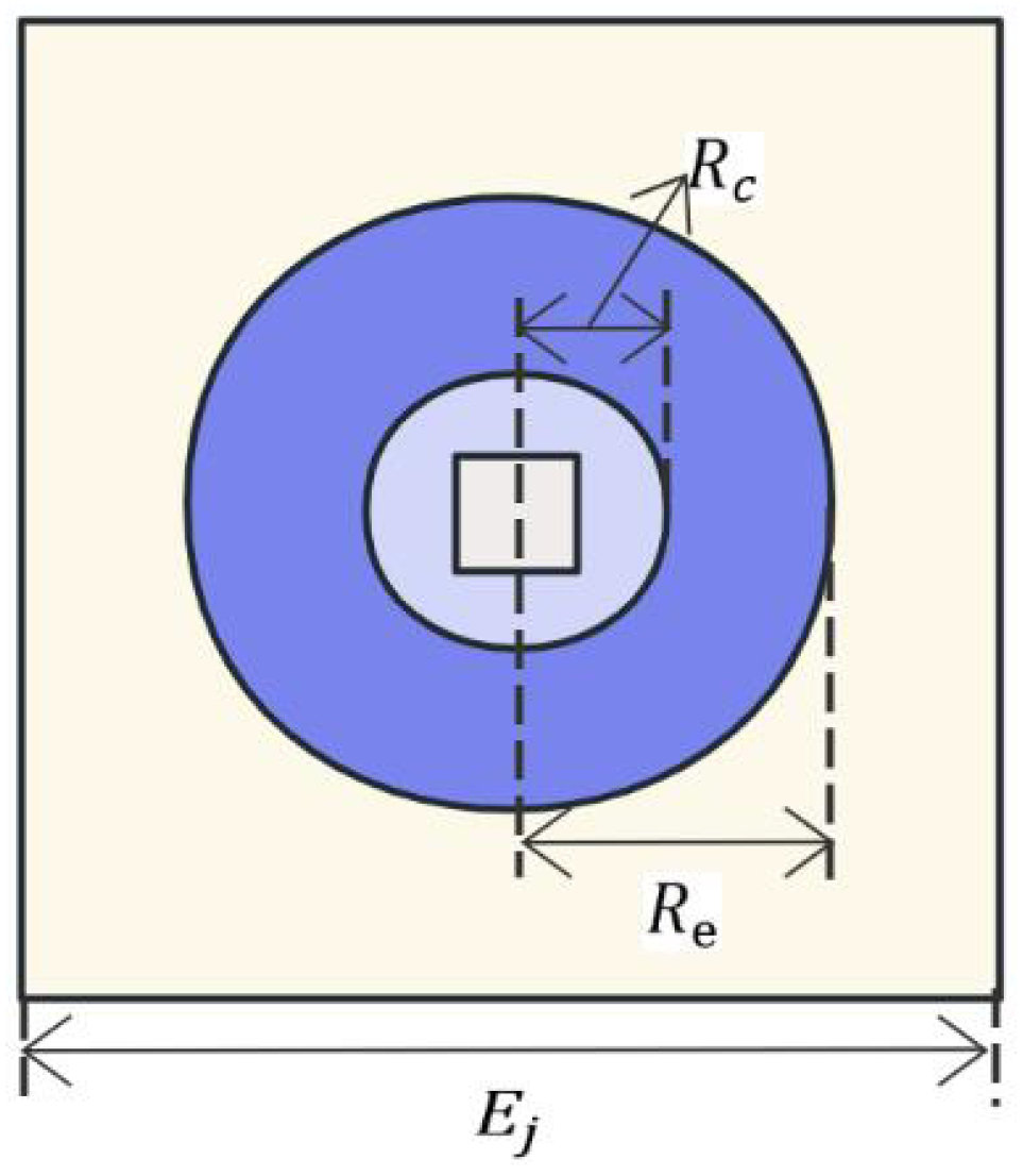
During search movement, the robot must maneuver around obstacles and other robots. Each robot maintains a local map centered on itself and continuously updates this map as it moves. The size of the local map is determined by E j . The robot and obstacle create a collision zone that extends outward, denoted by R c . An expansion area is established outside of the robot’s collision zone, and its size determined by R e , as illustrated in Figure 5 and Figure 6. To avoid obstacles, the robot plans its path by referencing its local map and adjusting to changes in the expansion zone as obstacles emerge. Unreachable positions occur if they fall within the robot’s collision zone. Throughout the simulation process, the local map size for E j is set to 3 m, the collision zone is set to 0.15 m with R c , while the expansion radius is adjusted to 1 m with R e . Figure 7 displays the simulation’s impact on the environment. The local map size maintained by each robot appears as a red boxed area.

3.5. Evaluation Index

The introduced concept here is the smallest enclosing circle, which refers to the smallest circle that can enclose a group of points on the plane. Once robots are grouped, the center and radius of the smallest enclosing circle are calculated for each robot group. If there is only one robot in the current group, the radius of the smallest circle is set to the robot’s radius. The average radius, denoted by R a , is then calculated using the radius of the smallest enclosing circle for all groups, and is only calculated when it has been found. A target is deemed found when the distance tolerance d t between the actual target position and final convergence position of the robots is within 0.5 m. Another evaluation index is the success rate, which is calculated as the ratio of the number of successful experiments to the total number of experiments, and it is indicated by the variable S R . An experiment is marked as successful if the robot population successfully searches all targets.

4. Wilcoxson Rank Sum Test and Comparative Experiment

4.1. Wilcoxson Rank Sum Test

Three representative benchmark test questions and their variants are given in Table 1. The historical optimal weight grey wolf optimization algorithm solves the aforementioned representative benchmark problems to test whether the proposed algorithm has search bias.
In the test, each problem is repeatedly solved over 30 times by 1000 iterations with 30 search agents. The shifting of the global optimal point is taken as the test factor. Table 2 reports the Wilcoxon rank sum test results. In the table, the middle two columns show the average error of each original benchmark function and its shifted variants, respectively; the last column shows the corresponding p-values. As shown in the table, all p-values are well above the 5% level of significance. The comprehensive p-value, p = P r e j e c t H 0 | H 0 i s t r u e = 1 1 0.9512 * 1 0.6894 * 1 0.2213 = 0.9882 > 0.5 . Therefore, we cannot reject the null hypothesis (H0) that the average error of the original benchmark function is equal to the average error of the shifted variants. In other words, the test results statistically verify that the historical optimal weight grey wolf optimization algorithm has no search bias for the origin of the coordinate system.

4.2. Experimental Environment

In the comparative experiment, the CEC 2017 test suite is employed. This test suite includes 3 unimodal functions, 7 simple multi-modal functions, 10 hybrid functions, and 10 compositional functions, and all are randomly shifted, with the first 10 functions also rotated. For the sake of fairness, all comparison algorithms were stopped after reaching the maximum number of functions evaluated; NFE = 1000. Other original parameter settings for competing algorithms were adopted in the experiment. Each comparative group was independently run over 30 times on a computer with a 2.3 GHz CPU and 32 GB of RAM.

4.3. Results and Discussion

Table 3 shows the average error and standard deviation of these competing algorithms when solving the 30-dimensional CEC 2017 test function using 30 search agents. In Table 3, the first column lists the sequence of 30 benchmark functions in the CEC 2017 test suite; the next four columns show the results obtained by the four competing algorithms, GWO, PSO, EGWO, and HOWGWO, respectively. The minimum average error in each comparison group is highlighted in bold.
As shown in Table 3, the EGWO algorithm obtained slightly better results for solving functions 6, 7, 9, 12, 16, 20, 25, and 26. However, the GWO and PSO algorithms failed to obtain smaller errors for all functions, and this poor performance can be attributed to the fact that both algorithms have search bias for the coordinate origin, while the functions in the CEC 2017 test suite are randomly shifted. If we rank these competing algorithms in ascending order of the average error of each test function and then sum these ranks, we obtain 90(GWO), 120(PSO), 51(EGWO), and 39(HOWGWO), respectively, where we can see that the summation of the HOWGWO algorithm is minimal. This also shows that the performance of the algorithm proposed in this paper is excellent in solving real-parameter numerical optimization problems in the CEC 2017 suite.
Multiple comparison tests were conducted to test the significance of the difference between the performance of the proposed HOWGWO algorithm and other competing algorithms. The p-value of Friedman’s test is equal to 3.89 × 10 17 on the 30-dimensional suite. This indicates that the efficiency of all competing algorithms differs significantly. Furthermore, Bonferroni’s test was performed to detect concrete performance differences between the compared algorithms. The post-hoc test results of the proposed HOWGWO algorithm against algorithms GWO, PSO, and EGWO are 1.91 × 10 6 , 2.59 × 10 7 , and 6.1 × 10 3 , which are less than the 0.05 significance level. The statistical results show that the proposed HOWGWO algorithms all significantly outperform the competing algorithms for solving the 30-dimensional benchmark suite.
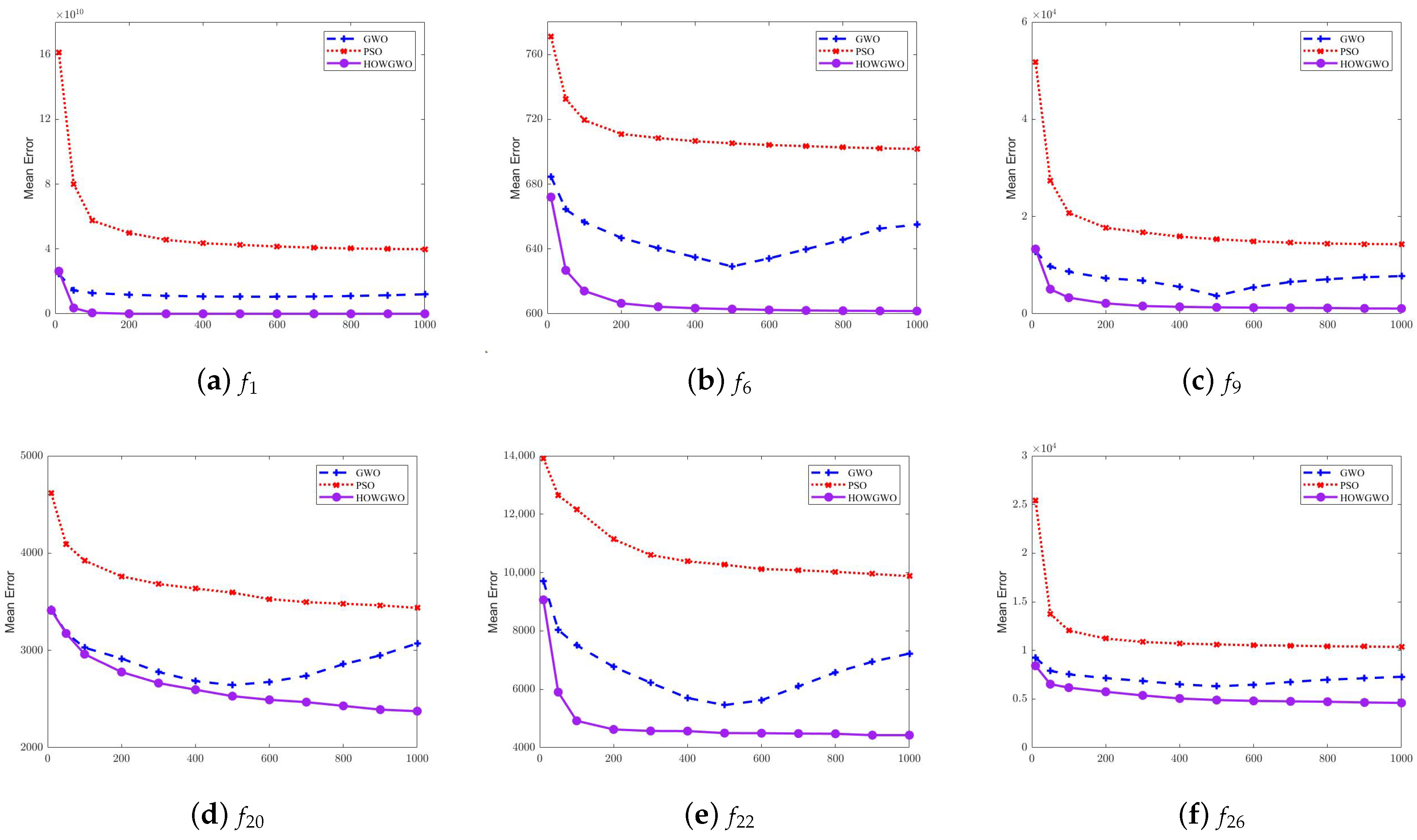
Figure 8 visually displays the performance differences between the algorithms. The figure plots the average convergence of each competing algorithm over 30 independent runs for a number of selected functions. The horizontal axis is the number of times the function was evaluated, and the vertical axis is the average of the errors. In Figure 8, the algorithms GWO, PSO, and HOWGWO are indicated by the blue dashed line marked with a plus sign, the red dashed line with the cross mark, and the purple solid line with the circle mark, respectively. The x-axis records the number of times the function was evaluated, and the y-axis is the average error. To reduce the complexity of the figure, we show the average error of these convergence curves at the points [0.01, 0.05, 0.1, 0.2, 0.3, 0.4, 0.5, 0.6, 0.7, 0.8, 0.9, 1.0]*NFE, where NFE is the maximum number of function evaluations. Thus, each curve has 12 marked points. As illustrated in the figure, the average convergence speed of the HOWGWO algorithm is significantly better than that of its competitors, especially in solving certain functions (e.g., 6 and 22), where the proposed algorithm can converge to the optimal solution faster. This superior performance can mainly be attributed to the fact that the leader wolf uses the historical optimal positions of all individual grey wolves through Equation (17) to make an effective estimate of the location of the prey, and this estimated position is closer to the global optimal solution.

5. Simulation and Discussion of Results

5.1. Description of Relevant Parameters and Objective Function

Assuming that swarm robots search for four static unknown targets within a confined plane area, the targets’ positions are 5 , 6 , 4 , 3 , 1 , 5 , and 6 , 3 with a signal strength radius around 1.5 m. The simulation parameters are shown in Table 4. The objective function is given as follows:
f ( x ) = 1 , c o u n t ( P ) N r 0 , c o u n t ( P ) < N r
where P denotes the set of targets that the algorithm finally determines, c o u n t ( · ) is a function that finds the number of elements in the set, and N r denotes the actual number of targets.
P = p i r j P r , d p i , r j < d t
where P r denotes the set of real targets, d ( p i , r j ) represents the Euclidean distance between the real targets and the targets determined by the algorithm, and d t is the distance threshold.

5.2. Search Process of Robots

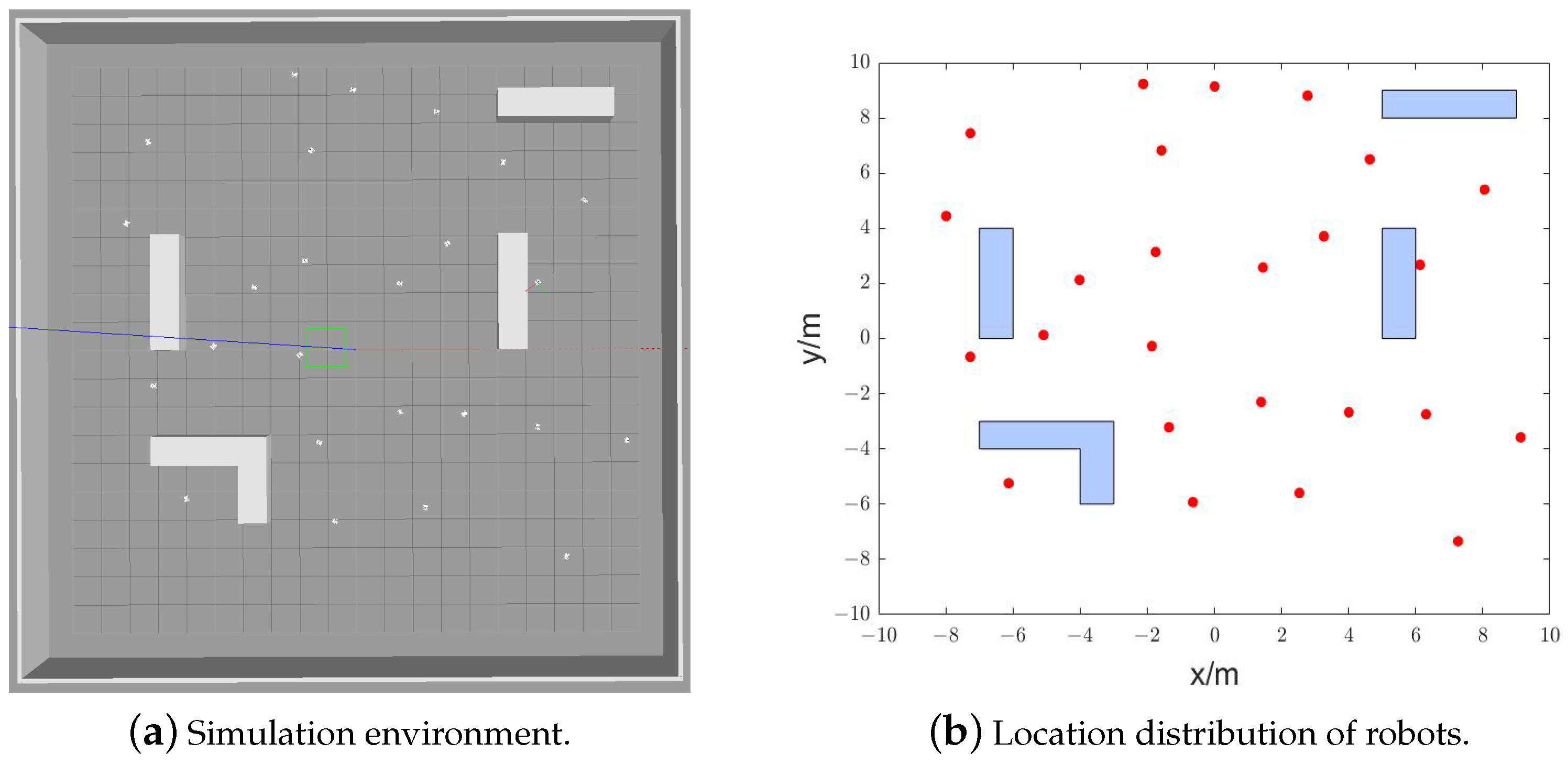
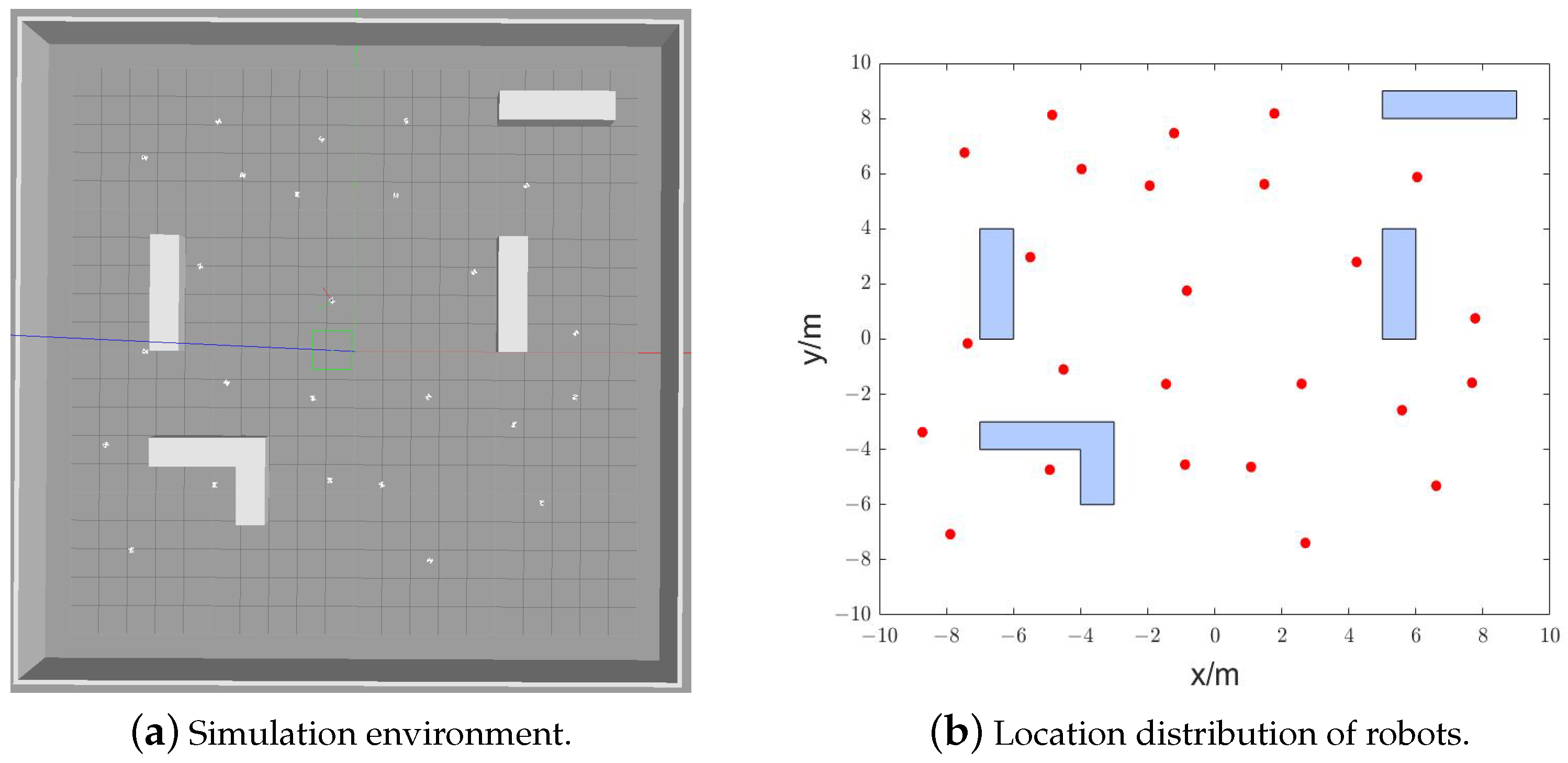
The process of searching for targets in an unknown environment with the help of 25 robots is illustrated in Figure 9, Figure 10, Figure 11 and Figure 12. In Figure 9, the robots were initialized with random positions outside the obstacle occupancy. Figure 10 depicts the search behaviors of the robots in the first stage, and Figure 11 illustrates various groups of robots by employing distinct symbols, such as ▴, ▾, ★ and •, in the second stage. Finally, the outcome of the search is illustrated in Figure 12. Here, ‘◯’ denotes the actual positions of the targets, while ‘▽’ represents the aggregated positions of the grouped robots (i.e., the positions of the targets determined by the robots). It is apparent from the figure that the aggregated positions of the grouped robots overlap closely with the actual positions of the targets.

5.3. Results and Discussion

Here, 50 independent runs were conducted for every parameter group, and the percentage of the targets found and the average radius, R a , for the smallest enclosing circle are documented. The outcomes of the parameter adjustments on simulation results are presented in Table 5, Table 6 and Table 7.
The data presented in Table 5 indicate a positive correlation between the number of iterations and the success rate of the robots in locating all targets. The average value of R a exhibits minimal changes throughout the process. The success rate of the target search tends to increase and decrease with the percentage factor η , despite keeping the total number of iterations constant. This suggests that appropriately adjusting η for the first stage iterations can improve the success rate. To expand, robots randomly explore and gather information during the first stage, and the grey wolf optimization utilizes these data to create optimal historical weights in the second stage, which eventually become the foundation for grouping. Unfortunately, as η increases, the robots in the second stage do not go through enough iterations to converge to the target’s vicinity. Consequently, the robots fail to locate the target, and the success rate shows a trend of increasing, then decreasing.
Table 6 presents the findings of our simulation experiments conducted with varying threshold values of f t h . The findings reveal that a higher f t h results in a significant decrease in the success rate of the target search. This outcome is due to the robots’ grouping strategy during the second stage, which relies on SAPs’ direction. In this strategy, the initial SAPs’ accuracy depends on data collected in the first stage. A high f t h value leads to the filtering of most target data collected in the first stage, resulting in generating inaccurate SAPs that deviate from the actual targets. Therefore, the absence of SAPs leads to the failure to locate all targets. Alternatively, a smaller f t h value enables the use of more data on the historical optimal position of the robots, which facilitates generating accurate SAPs around all targets, resulting in the increased success rate of the target search.
The results presented in Table 5 and Table 6 indicate that both parameters η and f t h have significant effects on the outcomes of the experiment. Between them, the parameter η controls the ratio of iterations of the two stages that comprise the algorithm. A smaller η means that the second stage has enough iterations for a group search, but the first stage might not offer effective global information for the second stage; a larger η will result in the second stage not having enough iterations to converge to the targets, thus failing to obtain accurate target locations. Parameter f t h , on the other hand, mostly influences the algorithm’s performance in the second stage. A smaller f t h retains more historical location information, which can be beneficial to SAP generation but which increases the computation; a larger f t h may filter out more useful location information, resulting in the algorithm’s inability to generate valid SAPs and decreasing its accuracy.
Table 7 shows the success rates of the Historical Optimal Weighting Grey Wolf Optimization (HOWGWO) and the Constriction Factor Particle Swarm Optimization (CFPSO) based on a grouping strategy [25] for target search in the same simulation environment. In this context, S R g represents the success rate of target search in HOWGWO, and S R p represents the success rate of target searching in CFPSO.
The success rate of the proposed algorithm, S R g , is significantly higher than that of the previous algorithm, S R p . Particularly when the number of robots is less than 30, S R g is more than three times higher than S R p . This indicates that the proposed algorithm lowers the required number of robots while maintaining a high success rate. Consequently, the proposed algorithm improves the search efficiency.

6. Conclusions

In this paper, we propose a Historical Optimal Weighing Grey Wolf Optimization (HOWGWO) algorithm based on an improved grouping strategy. In comparison with the original Grey Wolf Optimization (GWO) algorithm, the proposed algorithm emphasizes the wolf leadership hierarchy using the historical optimal weight, dynamically estimates the potential location of prey, and guides each wolf to move toward the estimated location of prey. Then, the improved grouping strategy allows the algorithm to dynamically adjust the number of groups during the grouping stage. The results of statistical analysis show that this position updating strategy produces no substantial search bias on the coordinate origin. Furthermore, the CEC 2017 test suite comparison findings reveal that the algorithm has considerable advantages in terms of convergence speed and solution quality. Meanwhile, the test results in the simulation environment show that varied parameter settings have a significant impact on the success rate of solving the multiple targets search problems. Within a suitable range of parameters, the algorithm proposed in this research can successfully be applied to the optimization of multiple target search problems for swarm robots. Future study will concentrate on making the strategy applicable to more complex situations and for real physical robots. Furthermore, solving the problem of boosting the exploitation capability of HOWGWO without compromising its exploration capability is an important research path. Moreover, the improved grouping strategy could be considered as a reference for developing the multi-objective version of the metaheuristic algorithm.

Author Contributions

Y.L.: Conceptualization, methodology, software, validation, formal analysis, investigation, data curation, writing—original draft preparation, writing—review and editing, visualization; Q.Z.: Conceptualization, methodology, resources, supervision, funding acquisition; Z.Z.: data curation. All authors have read and agreed to the published version of the manuscript.

Funding

National Natural Science Foundation of China (61902057, 62276058, 41774063), Fundamental Research Funds for the Central Universities (N2317003, N2217003).

Institutional Review Board Statement

Not applicable.

Informed Consent Statement

Not applicable.

Data Availability Statement

Not applicable.

Acknowledgments

We would like to thank the anonymous reviewers for their careful reading and useful comments that helped us improve the final version of this paper.

Conflicts of Interest

There are no conflicts of interest regarding the publication of this paper.

References

  1. Chen, J.R.; Wang, J.J.; Hou, X.W.; Fang, Z.R.; Du, J.; Ren, Y. Advance into ocean: From bionic monomer to swarm intelligence. Acta Electron. Sin. 2021, 49, 2458–2467. [Google Scholar]
  2. Prelec, D.; Seung, H.S.; McCoy, J. A solution to the single-question crowd wisdom problem. Nature 2017, 541, 532–535. [Google Scholar] [CrossRef]
  3. Berdahl, A.; Torney, C.J.; Ioannou, C.C.; Faria, J.J.; Couzin, I.D. Emergent sensing of complex environments by mobile animal groups. Science 2013, 339, 574–576. [Google Scholar] [CrossRef] [Green Version]
  4. Eiben, A.E.; Smith, J. From evolutionary computation to the evolution of things. Nature 2015, 521, 476–482. [Google Scholar] [CrossRef] [PubMed]
  5. Deng, L.X. Study on multiple mobile robots coordinated planning algorithms. Ph.D. Thesis, Shandong University, Jinan, China, 2016. [Google Scholar]
  6. Sharma, S.; Shukla, A.; Tiwari, R. Multi robot area exploration using nature inspired algorithm. Biol. Inspired Cogn. Archit. 2016, 18, 80–94. [Google Scholar] [CrossRef]
  7. Mehfuz, F. Recent implementations of autonomous robotics for space exploration. In Proceedings of the 2018 International Conference on Sustainable Energy, Electronics, and Computing Systems (SEEMS), Greater Noida, India, 26–27 October 2018; pp. 1–6. [Google Scholar]
  8. St-Onge, D.; Kaufmann, M.; Panerati, J.; Ramtoula, B.; Cao, Y.J.; Coffey, E.B.J.; Beltrame, G. Planetary exploration with robot teams: Implementing higher autonomy with swarm intelligence. IEEE Robot. Autom. Mag. 2020, 27, 159–168. [Google Scholar] [CrossRef]
  9. Duarte, M.; Gomes, J.; Costa, V.; Rodrigues, T.; Silva, F.; Lobo, V.; Marques, M.M.; Oliveira, S.M.; Christensen, A.L. Application of swarm robotics systems to marine environmental monitoring. In Proceedings of the OCEANS 2016, Shanghai, China, 10–13 April 2016; pp. 1–8. [Google Scholar]
  10. Pan, J.f.; Zi, B.; Wang, Z.Y.; Qian, S.; Wang, D.M. Real-time dynamic monitoring of a multi-robot cooperative spraying system. In Proceedings of the 2019 IEEE International Conference on Mechatronics and Automation (ICMA), Tianjin, China, 4–7 August 2019; pp. 862–867. [Google Scholar]
  11. Elwin, M.L.; Freeman, R.A.; Lynch, K.M. Distributed environmental monitoring with finite element robots. IEEE Trans. Robot. 2020, 36, 380–398. [Google Scholar] [CrossRef]
  12. Bakhshipour, M.; Ghadi, M.J.; Namdari, F. Swarm robotics search & rescue: A novel artificial intelligence-inspired optimization approach. Appl. Soft Comput. 2017, 57, 708–726. [Google Scholar]
  13. Din, A.; Jabeen, M.; Zia, K.; Khalid, A.; Saini, D.K. Behavior-based swarm robotic search and rescue using fuzzy controller. Comput. Electr. Eng. 2018, 70, 53–65. [Google Scholar] [CrossRef]
  14. Cardona, G.A.; Calderon, J.M. Robot swarm navigation and victim detection using rendezvous consensus in search and rescue operations. Appl. Sci. 2019, 9, 1702. [Google Scholar] [CrossRef] [Green Version]
  15. Yang, B.; Ding, Y.S.; Jin, Y.C.; Hao, K.R. Self-organized swarm robot for target search and trapping inspired by bacterial chemotaxis. Robot. Auton. Syst. 2015, 72, 83–92. [Google Scholar] [CrossRef]
  16. Megalingam, R.K.; Nagalla, D.; Kiran, P.R.; Geesala, R.T.; Nigam, K. Swarm based autonomous landmine detecting robots. In Proceedings of the 2017 International Conference on Inventive Computing and Informatics (ICICI), Coimbatore, India, 23–24 November 2017; pp. 608–612. [Google Scholar]
  17. Tarapore, D.; Gross, R.; Zauner, K.-P. Sparse robot swarms: Moving swarms to real-world applications. Front. Robot. AI 2020, 57, 83. [Google Scholar] [CrossRef] [PubMed]
  18. Albiero, D.; Pontin Garcia, A.; Kiyoshi Umezu, C.; Leme de Paulo, R. Swarm robots in mechanized agricultural operations: A review about challenges for research. Comput. Electron. Agric. 2022, 193, 106608. [Google Scholar] [CrossRef]
  19. Senanayake, M.; Senthooran, I.; Barca, J.C.; Chung, H.; Kamruzzaman, J.; Murshed, M. Search and tracking algorithms for swarms of robots: A survey. Robot. Auton. Syst. 2016, 75, 422–434. [Google Scholar] [CrossRef]
  20. Prodhon, C. A hybrid evolutionary algorithm for the periodic location-routing problem. Eur. J. Oper. Res. 2011, 210, 204–212. [Google Scholar] [CrossRef]
  21. Zheng, Z.; Tan, Y. Group explosion strategy for searching multiple targets using swarm robotic. In Proceedings of the 2013 IEEE Congress on Evolutionary Computation, Cancun, Mexico, 20–23 June 2013; pp. 821–828. [Google Scholar]
  22. Liu, R.C.; Niu, X.; Jiao, L.C.; Ma, J.J. A multi-swarm particle swarm optimization with orthogonal learning for locating and tracking multiple optimization in dynamic environments. In Proceedings of the 2014 IEEE Congress on Evolutionary Computation (CEC), Beijing, China, 6–11 July 2014; pp. 754–761. [Google Scholar]
  23. Dadgar, M.; Jafari, S.; Hamzeh, A. A PSO-based multi-robot cooperation method for target searching in unknown environments. Neurocomputing 2016, 177, 62–74. [Google Scholar] [CrossRef]
  24. Tang, H.W.; Sun, W.; Yu, H.S.; Lin, A.P.; Xue, M.; Song, Y.X. A novel hybrid algorithm based on PSO and FOA for target searching in unknown environments. Appl. Intell. 2019, 49, 2603–2622. [Google Scholar] [CrossRef]
  25. Zedadra, O.; Guerrieri, A.; Seridi, H. LFA: A Lévy Walk and Firefly-Based Search Algorithm: Application to Multi-Target Search and Multi-Robot Foraging. Big Data Cogn. Comput. 2022, 6, 22. [Google Scholar] [CrossRef]
  26. Ariyarit, A.; Kanazaki, M.; Bureerat, S. An Approach Combining an Efficient and Global Evolutionary Algorithm with a Gradient-Based Method for Airfoil Design Problems. Smart Sci. 2020, 8, 14–23. [Google Scholar] [CrossRef]
  27. Nadimi-Shahraki, M.H.; Zamani, H.; Fatahi, A.; Mirjalili, S. MFO-SFR: An Enhanced Moth-Flame Optimization Algorithm Using an Effective Stagnation Finding and Replacing Strategy. Mathematics 2023, 11, 862. [Google Scholar] [CrossRef]
  28. Tang, Q.R.; Ding, L.; Yu, F.C.; Zhang, Y.; Li, Y.H.; Tu, H.B. Swarm robots search for multiple targets based on an improved grouping strategy. IEEE/ACM Trans. Comput. Biol. Bioinform. 2018, 15, 1943–1950. [Google Scholar] [CrossRef] [PubMed]
  29. Mirjalili, S.; Mirjalili, S.M.; Lewis, A. Grey wolf optimizer. Adv. Eng. Softw. 2014, 69, 46–61. [Google Scholar] [CrossRef] [Green Version]
  30. Kennedy, J.; Eberhart, R. Particle swarm optimization. In Proceedings of the ICNN’95-International Conference on Neural Networks, Perth, Australia, 27 November–1 December 1995; pp. 1942–1948. [Google Scholar]
  31. Luo, K.P. Enhanced grey wolf optimizer with a model for dynamically estimating the location of the prey. Appl. Soft Comput. 2019, 77, 225–235. [Google Scholar] [CrossRef]
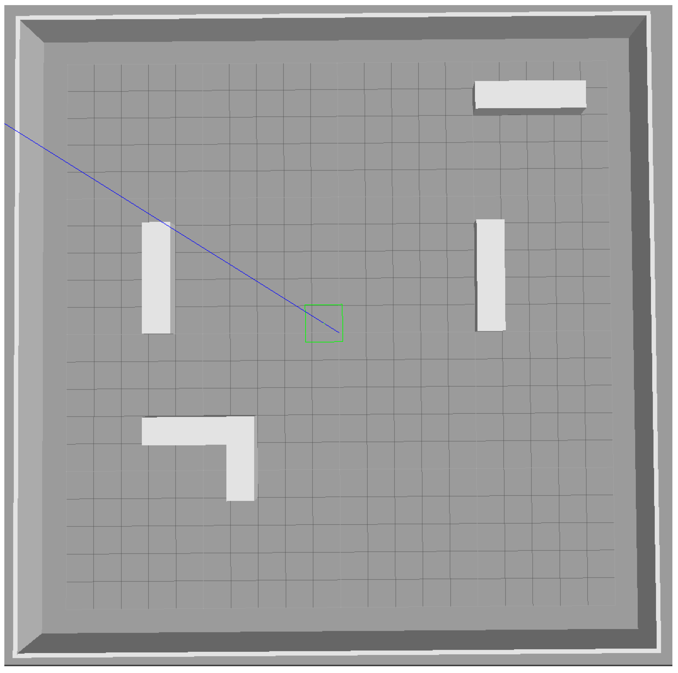
Figure 1. The search area and polygon obstacles.
Mathematics 11 02630 g001
Figure 2. Target signal strength distribution.
Mathematics 11 02630 g002
Figure 3. Five separate candidate positions generated by the random walk stage.
Mathematics 11 02630 g003
Figure 4. The complete algorithm flow chart.
Mathematics 11 02630 g004
Figure 5. Expansion zone and collision zone local map of the robot.
Mathematics 11 02630 g005
Figure 6. Collision area of obstacle.
Mathematics 11 02630 g006
Figure 7. Local map of the robot in simulation.
Mathematics 11 02630 g007
Figure 8. Average convergence graphs of competing algorithms: GWO, PSO, and HOWGWO on some selected 30-dimensional functions over 30 independent runs.
Mathematics 11 02630 g008
Figure 9. Iteration = 1, robots are distributed randomly.
Mathematics 11 02630 g009
Figure 10. Iteration = 20, robots move randomly.
Mathematics 11 02630 g010
Figure 11. Iteration = 40, robots are grouped.
Mathematics 11 02630 g011
Figure 12. Iteration = 100, robots converge near the target points.
Mathematics 11 02630 g012
Table 1. Three representative benchmark functions.
FunctionRange
f a x = i = 1 n x i 2 [ 10 , 100 ]
f a s x = i = 1 n x i 0.0001 2 [ 10 , 100 ]
f b x = i = 1 n j = 1 i x i 2 [ 100 , 10 ]
f b s x = i = 1 n j = 1 i x i 0.01 2 [ 100 , 10 ]
f c x = i = 1 n x i 2 10 cos 2 i + 10 [ 5.12 , 5.12 ]
f c s x = i = 1 n x i 1 2 10 cos 2 π x i 1 + 10 [ 6.12 , 4.12 ]
Table 2. Wilcoxon rank sum test of the function shifting effect on the performances of the historical optimal weighting grey wolf optimization.
FunctionMean Error—OriginalMean Error—Shiftedp-Value
Sphere 1.47 × 10 14 1.17 × 10 14 0.9512
Schwdfel 1.2 3.41 × 10 1 3.61 × 10 1 0.6894
Rastrign 4.27 × 10 1 3.79 × 10 1 0.2213
Table 3. Mean errors and standard deviations (±std) on CEC 2017 test functions with dimension n = 30.
Func.GWOPSOEGWOHOWGWO
1 1.20 × 10 10 ( 4.33 × 10 9 ) 3.98 × 10 10 ( 1.47 × 10 10 ) 4.76 × 10 3 ( 5.48 × 10 3 ) 2 . 83 × 10 3 ( 3 . 47 × 10 3 )
2 4.73 × 10 35 ( 1.85 × 10 36 ) 1.26 × 10 53 ( 6.89 × 10 53 ) 1.78 × 10 18 ( 6.04 × 10 18 ) 1 . 56 × 10 18 ( 5 . 95 × 10 18 )
3 2.81 × 10 5 ( 8.60 × 10 5 ) 1.20 × 10 5 ( 1.71 × 10 4 ) 5.10 × 10 4 ( 1.53 × 10 4 ) 5 . 94 × 10 4 ( 1 . 29 × 10 4 )
4 1.90 × 10 3 ( 1.30 × 10 3 ) 9.60 × 10 3 ( 5.36 × 10 3 ) 4.92 × 10 2 ( 2.10 × 10 1 ) 4 . 88 × 10 2 ( 1 . 78 × 10 1 )
5 8.10 × 10 2 ( 2.51 × 10 1 ) 9.35 × 10 2 ( 2.83 × 10 1 ) 6.68 × 10 2 ( 6.80 × 10 1 ) 6 . 46 × 10 2 ( 6 . 62 × 10 1 )
6 6.55 × 10 2 ( 8.95 × 10 0 ) 7.01 × 10 2 ( 1.10 × 10 1 ) 6 . 01 × 10 2 ( 1 . 10 × 10 0 ) 6.02 × 10 2 ( 1.17 × 10 0 )
7 1.16 × 10 3 ( 7.07 × 10 1 ) 1.43 × 10 3 ( 8.99 × 10 1 ) 9 . 06 × 10 2 ( 6 . 82 × 10 1 ) 9.11 × 10 2 ( 6.79 × 10 1 )
8 1.04 × 10 3 ( 2.48 × 10 1 ) 1.17 × 10 3 ( 2.10 × 10 1 ) 9.60 × 10 2 ( 6.10 × 10 1 ) 9 . 59 × 10 2 ( 6 . 84 × 10 1 )
9 7.75 × 10 3 ( 2.46 × 10 3 ) 1.43 × 10 4 ( 1.37 × 10 3 ) 1 . 08 × 10 3 ( 2 . 79 × 10 2 ) 1.08 × 10 3 ( 2.84 × 10 2 )
10 8.32 × 10 3 ( 7.40 × 10 2 ) 1.02 × 10 4 ( 2.52 × 10 2 ) 8.43 × 10 3 ( 5.16 × 10 2 ) 8 . 33 × 10 3 ( 8 . 21 × 10 2 )
11 5.18 × 10 3 ( 1.36 × 10 3 ) 9.37 × 10 3 ( 2.45 × 10 3 ) 1.23 × 10 3 ( 5.25 × 10 1 ) 1 . 21 × 10 3 ( 6 . 15 × 10 1 )
12 1.31 × 10 9 ( 1.23 × 10 9 ) 1.05 × 10 10 ( 6.79 × 10 9 ) 5 . 04 × 10 5 ( 6 . 00 × 10 5 ) 7.02 × 10 5 ( 6.19 × 10 5 )
13 6.16 × 10 8 ( 4.94 × 10 8 ) 7.88 × 10 9 ( 1.01 × 10 10 ) 1.51 × 10 4 ( 1.55 × 10 4 ) 1 . 51 × 10 4 ( 1 . 43 × 10 4 )
14 2.29 × 10 6 ( 1.27 × 10 6 ) 8.12 × 10 6 ( 1.10 × 10 7 ) 3.80 × 10 4 ( 3.19 × 10 4 ) 2 . 68 × 10 4 ( 2 . 47 × 10 4 )
15 2.27 × 10 7 ( 2.27 × 10 7 ) 3.31 × 10 8 ( 2.86 × 10 8 ) 9.66 × 10 3 ( 8.23 × 10 3 ) 8 . 68 × 10 3 ( 7 . 95 × 10 3 )
16 3.97 × 10 3 ( 3.93 × 10 2 ) 6.03 × 10 3 ( 1.15 × 10 3 ) 2.98 × 10 3 ( 5.03 × 10 2 ) 2 . 89 × 10 3 ( 5 . 66 × 10 2 )
17 2.84 × 10 3 ( 2.49 × 10 2 ) 5.99 × 10 3 ( 9.58 × 10 3 ) 1 . 97 × 10 3 ( 2 . 02 × 10 2 ) 2.05 × 10 3 ( 1.92 × 10 2 )
18 2.18 × 10 7 ( 2.52 × 10 7 ) 7.26 × 10 7 ( 8.67 × 10 7 ) 9.16 × 10 5 ( 1.19 × 10 6 ) 8 . 38 × 10 5 ( 8 . 34 × 10 5 )
19 9.13 × 10 7 ( 1.37 × 10 8 ) 4.71 × 10 8 ( 7.90 × 10 8 ) 1.41 × 10 4 ( 1.55 × 10 4 ) 1 . 10 × 10 4 ( 1 . 00 × 10 4 )
20 3.07 × 10 3 ( 2.10 × 10 2 ) 3.44 × 10 3 ( 7.65 × 10 1 ) 2 . 30 × 10 3 ( 2 . 43 × 10 2 ) 2.37 × 10 3 ( 2.54 × 10 2 )
21 2.58 × 10 3 ( 2.99 × 10 1 ) 2.73 × 10 3 ( 5.21 × 10 1 ) 2.47 × 10 3 ( 6.20 × 10 1 ) 2 . 46 × 10 3 ( 4 . 77 × 10 1 )
22 7.23 × 10 3 ( 2.78 × 10 3 ) 9.88 × 10 3 ( 9.28 × 10 2 ) 5.85 × 10 3 ( 3.63 × 10 3 ) 4 . 43 × 10 3 ( 3 . 32 × 10 3 )
23 3.10 × 10 3 ( 4.85 × 10 1 ) 3.62 × 10 3 ( 2.32 × 10 2 ) 2.76 × 10 3 ( 6.81 × 10 1 ) 2 . 75 × 10 3 ( 6 . 45 × 10 1 )
24 3.27 × 10 3 ( 5.07 × 10 1 ) 4.01 × 10 3 ( 4.41 × 10 2 ) 3.01 × 10 3 ( 3.68 × 10 1 ) 3 . 00 × 10 3 ( 5 . 38 × 10 1 )
25 3.30 × 10 3 ( 1.93 × 10 2 ) 4.44 × 10 3 ( 8.86 × 10 2 ) 2 . 90 × 10 3 ( 1 . 44 × 10 1 ) 2.89 × 10 3 ( 1.78 × 10 1 )
26 7.29 × 10 3 ( 7.90 × 10 2 ) 1.04 × 10 4 ( 1.08 × 10 3 ) 4 . 24 × 10 3 ( 5 . 66 × 10 2 ) 4.60 × 10 3 ( 6.86 × 10 2 )
27 3.48 × 10 3 ( 1.10 × 10 2 ) 4.65 × 10 3 ( 4.68 × 10 2 ) 3.23 × 10 3 ( 1.44 × 10 1 ) 3 . 23 × 10 3 ( 1 . 43 × 10 1 )
28 4.15 × 10 3 ( 4.30 × 10 2 ) 6.55 × 10 3 ( 1.49 × 10 3 ) 3.22 × 10 3 ( 1.96 × 10 1 ) 3 . 22 × 10 3 ( 3 . 03 × 10 1 )
29 5.07 × 10 3 ( 3.84 × 10 2 ) 1.30 × 10 4 ( 3.05 × 10 4 ) 3.65 × 10 3 ( 2.20 × 10 2 ) 3 . 64 × 10 3 ( 1 . 52 × 10 2 )
30 1.31 × 10 8 ( 6.35 × 10 7 ) 1.31 × 10 9 ( 1.84 × 10 9 ) 9.20 × 10 3 ( 3.04 × 10 3 ) 8 . 51 × 10 3 ( 3 . 02 × 10 3 )
Table 4. Simulation parameters.
NameDescriptionValue
NSum of the Robots25
N i Maximum Iterations100
η Percentage Factor of Iterations0.4
f t h Grouping Threshold0.09
l d Distance Threshold3
L x × L y Search Range 20 × 20 ( m 2 )
Table 5. Effects of parameter ( N i , η ) change.
N N i η f th SR ( % ) Average of R a
251000.20.09940.55
251000.40.09980.47
251000.60.091000.53
251000.80.09960.65
251000.90.09882.29
25800.20.09900.46
25800.40.09940.50
25800.60.091000.58
25800.80.09940.94
25800.90.09762.10
25500.20.09880.79
25500.40.09920.53
25500.60.09960.44
25500.80.09882.27
25500.90.09643.17
Table 6. Effects of parameter f t h change.
N N i η f th SR ( % ) Average of R a
25800.40.09960.50
25800.40.50960.49
25800.41.00940.52
25800.41.50940.49
25800.42.00920.48
25800.42.50920.65
25800.43.00900.83
25800.43.50822.35
25800.44.00682.92
Table 7. Success rate in HOWGWO and CFPSO.
N N i η f th SR g ( % ) SR p ( % )
25800.10.099224
25800.20.099214
25800.30.099630
25800.40.099632
25800.40.209824
25800.40.309218
25800.40.409420
25800.40.509226
20800.40.099222
30800.40.099840
35800.40.099860
40800.40.0910064
Disclaimer/Publisher’s Note: The statements, opinions and data contained in all publications are solely those of the individual author(s) and contributor(s) and not of MDPI and/or the editor(s). MDPI and/or the editor(s) disclaim responsibility for any injury to people or property resulting from any ideas, methods, instructions or products referred to in the content.