
Dispatch for a Continuous-Time Microgrid Based on a Modified Differential Evolution Algorithm


1
School of Mathematics and Statistics, Chongqing Jiaotong University, Chongqing 400074, China
2
School of Mathematics, Southeast University, Nanjing 211189, China
*
Author to whom correspondence should be addressed.
Mathematics 2023, 11(2), 271; https://doi.org/10.3390/math11020271
Submission received: 5 December 2022
/
Revised: 1 January 2023
/
Accepted: 2 January 2023
/
Published: 4 January 2023
(This article belongs to the Special Issue Advances in Analysis and Application of Mathematical Optimization Algorithms)
Abstract
:The carbon trading mechanism is proposed to remit global warming and it can be considered in a microgrid. There is a lack of continuous-time methods in a microgrid, so a continuous-time model is proposed and solved by differential evolution (DE) in this work. This research aims to create effective methods to obtain some useful results in a microgrid. Batteries, microturbines, and the exchange with the main grid are considered. Considering carbon trading, the objective function is the sum of a quadratic function and an absolute value function. In addition, a composite electricity price model has been put forward to conclude the common kinds of electricity prices. DE is utilized to solve the constrained optimization problems (COPs) proposed in this paper. A modified DE is raised in this work, which uses multiple mutation and selection strategies. In the case study, the proposed algorithm is compared with the other seven algorithms and the outperforming one is selected to compare two different types of electricity prices. The results show the proposed algorithm performs best. The Wilcoxon Signed Rank Test is also used to verify its significant superiority. The other result is that time-of-use pricing (ToUP) is economic in the off-peak period while inclining block rates (IBRs) are economic in the peak and shoulder periods. The composite electricity price model can be applied in social production and life. In addition, the proposed algorithm puts forward a new variety of DE and enriches the theory of DE.
Keywords:
microgrid; carbon trading mechanism; electricity prices; constrained optimization problems (COPs); differential evolution (DE); constraint handling techniquesMSC:
90-08; 90-101. Introduction
Global warming leads to the rising of sea levels and the reduction of biological diversity. To cope with climate change, many countries have taken action, such as the promulgation of the Kyoto Protocol and the Paris Agreement. In addition, in the 21st century, carbon neutrality may become the leading global environmental goal [1]. However, in some countries, power system carbon emissions are still at a high level. Carbon emission is one of the main causes of global warming. Carbon is the fuel of microgrides, so it is required for microgrids to reduce carbon emissions. Many kinds of energy have been considered to generate electricity, including solar energy [2], wind energy [3] and nuclear energy [4].
Now, a lot of researchers have studied the optimization problems in microgrids. These articles have various objectives. The aim of [2] is to minimize the electricity cost and the battery operational cost. In addition, Ref. [3] intends to optimize the energy cost, carbon trading cost, and operational cost. Gholian et al. [5] is to maximize the profit. However, nearly all existing works use discrete-time models. Though they are effective for some problems, they can only give approximate results in some specific time points. There are some kinds of electricity prices, such as the time-of-use pricing in [2,3] and critical peak pricing in [6,7]. The time-of-use pricing changes the price depending on the load and critical peak pricing is similar to time-of-use pricing. Nevertheless, there is a deficiency summary in the studies of microgrids.
For optimization, there are various methods to deal with them. In [8], simulated annealing (SA) is applied to cope with the optimization problem in a smart grid. Ref. [9] utilizes mixed-integer linear programming (MILP) and genetic algorithm (GA) to optimize the unit commitment and economic dispatch in microgrids.
Differential evolution is also an ideal method to solve optimization problems. DE proved to be one of the most successful evolutionary algorithms for solving global optimization problems over continuous space during the past two decades [10]. In addition, Ref. [2] applied DE in the optimal dispatch of microgrids and made a great effect. Therefore, it is applied in this work. It has many modified types, such as MADE [11], MSIQDE [12], EMMSIQDE [13], C2oDE [14], ANDE [15], MVDE [16], FSTDE [17], UDE [18] and AGDE [19]. Mohamed et al. combine novel mutation methods with fitness-adaptive DE and adaptive guided DE in [20] and [21], respectively. Ref. [22] uses a shift mechanism in adaptive multiple-elites-guided composite DE. Hadi et al. propose success history-based differential evolution with linear population size reduction and semi-parameter adaptation (LSHADE-SPA) in [23] and find that this algorithm is competitive among other algorithms. Furthermore, [24] combines DE with Convolutional Neural Networks (CNNs). Numerical experiments indicate this method is vigorously competitive with the other 12 methods and it has high accuracy. In terms of mutation, [25] introduces many kinds of mutation strategies. Mohamed et al. propose new mutation strategies in [10,26].They estimate the proposed methods by some numerical experiments and find the superiority of the proposed methods. Moreover, in [2], DE/rand/1 and DE/current-to-best/1 are used for mutation. These research works are based on theoretical analysis and the results of case studies. They use valid methods, interpreting and presenting the results effectively. The authors’ perspectives are even-handed and they make use of all usable data. Therefore, their arguments and conclusions are convincing, and these works contribute to an understanding of the subject in a significant way. Nonetheless, nearly no research considers continuous-time models and algorithms in the optimal dispatch of microgrids, so their consequences will inevitably have some errors or deviations when considering the time points they do not select.
A DE algorithm needs to consider the constraints. There are three common methods: add constraints when it is initialization; use if statement after mutation and crossover; add penalty terms. In addition, using constraint handling techniques in selection is also optional. To deal with constraints, [2] use stochastic ranking (SR) and superiority of feasible solutions (SF) when selecting.
This work aims to build a continuous-time model and process different kinds of electricity prices. Then, design an effective algorithm to solve it. According to the above present situation, carbon trading is considered in this paper to build a continuous-time optimization model on a convex set. Then, a modified DE is proposed. Compared with [2], it uses DE/pbest/1 and DE/current-to-best/1 in mutation, and uses stochastic ranking (SR) and ε-constraint (EC) in selection. After that, eight kinds of DE algorithms are compared and it shows that the proposed algorithm is better than other algorithms. The Wilcoxon Signed Rank Test also demonstrates this result. Then, this algorithm is applied to study different electricity prices. We find that ToUP is economic in the off-peak period, but IBRs are economic in peak time and shoulder time. The main contributions of this study are as follows.
- Different from these existing works, this paper uses a continuous-time optimization model and uses the integral of time to replace the summation in existing works. Then the model is converted to an equivalent form that is easier to address. Compared to the discrete-time model, the constraint-time model is closer to reality and can give precise results at arbitrary required time points;
- Composite electricity price model is raised in this work. In this model, 5 types of electricity prices in [5] are summarized and represented by one equation in this work, so that future works can use this model to represent nearly all common types of electricity prices. Furthermore, it can provide convenience when comparing different electricity prices in simulation experiments;
- The mutation and the selection strategies of the DE algorithm in [2] are modified in this study. The simulation experiments suggest the proposed algorithm achieves more ideal results than the other seven mentioned algorithms. It converges fast and avoids premature convergence.
2. Modeling
2.1. Structure of Microgrid
Microgrids are usually equipped with batteries, microturbines, photovoltaic power generations, and wind power generations. They also exchange electricity with the main grid. It is a process by which they obtain energy. In addition, microgrids sell excess energy to the main grid. There are three types of load, which are industrial load, commercial load, and residential load. Demand response (DR) means that customers change their loads according to the electricity price or incentive mechanism. Microgrids reduce pollution and they use renewable energy such as solar and wind [27]. In this study, we mainly consider batteries, microturbines, and the exchange with the main grid. The structure of this microgrid is represented in Figure 1.
2.2. Thermal Power Units Operation
The fuel of the thermal power units is natural gas in this paper. The cost of natural gas is quadratic function of units output [16,28].
where denotes the power output of the thermal power units at time t and denote the fuel cost coefficients; and denote the minimum and maximum of the thermal power units’ power output, respectively; in addition, T is the end point of time.
2.3. Electricity Purchase
According to [28], the cost of electricity sold to the main grid can be ignored to simplify the model. These are five kinds of prices of electricity that are introduced in [5]. They are day-ahead pricing (DAP), time-of-use pricing (ToUP), peak pricing (PP), inclining block rates (IBRs), and critical peak price (CPP) [5]. In this work, they can be concluded as (3).
where is a Riemann integrable vector function which respresents the power of purchasing electricity at time t. Different components of mean different ranges of the power. In addition, is also a Riemann integrable vector function, respresenting the price of electricity and its different components mean different prices. The “·” operator means the inner product of two vectors.
In fact, as for five kinds of electricity prices, DAP is shown in (4), which is the simplest form of electricity prices. ToUP is a type of DAP [5]. In addition, CPP is a type of ToUP and the quantity of purchasing electricity and the price of electricity both can be considered as piecewise functions which are both in three segments. PP can be written as (5) and it has one more term than DAP. Furthermore, IBRs are introduced in (6).
where is the power of purchasing electricity at time t and is the threshold value at time t; , , and denote 3 kinds of electricity prices.
The quantity of purchasing electricity and the price of electricity for the first 3 kinds of electricity costs mentioned above are all one dimension, but for PP and IBRs, they become two dimensions. (5) can be written as (7).
where is equal to and is equal to . (6) can be written as (8).
where denotes the step function, which is
In (8), is equal to and is equal to , . Therefore, the first component is the part of power which is less than , while the last component is the part of power which is more than . For the reason that for every t in , it guarantees that the last component of equals to 0 until the first component reaches its upper bound in the optimization problem without adding extra constraints. If there are three or more kinds of electricity prices, the analogous method can be used.
Furthermore, the power of purchasing electricity should also be limited to a specific range.
where and denote the minimum and maximum of the ith component of , respectively.
2.4. Carbon Emission
The carbon emission quota is judged by the provincial carbon emissions trading authority, issued and allowed to include carbon emissions trading enterprises within a specific period of carbon dioxide emissions. The carbon emission quota at time t can be calculated as
where is the carbon emission coefficient per unit power.
Thermal power units are the major resource of carbon emission. The actual carbon emission at time t can be calculated as
where is the carbon emission intensity per unit output.
The carbon trading cost is
where is the carbon trading market price.
2.5. Battery Operation
The cost of the battery contains maintenance cost and depreciation cost.
where and denote the maintenance price and depreciation price, respectively. is the power of the battery at time t where indicates discharging while indicates charging. and denote the minimum and maximum of the battery’s power, respectively. is less than 0 while is more than 0.
2.6. Optimization Problem
The power researched in this work concludes the power output of the thermal power units, the power of purchasing electricity and the power of the battery.
where denotes the ith component of ; n denotes the dimension of ; denotes the load at time t.
In conclusion, the optimization problem is expressed as
where C is the total cost; denotes the cost of natural gas and ; denotes the cost of electricity bought from the main grid and ; denotes the fixed cost, which is the sum of other costs, including operating and maintenance costs, start-up and shut-down costs, and so on [28]. To be simplicity, is regarded as a constant. Furthermore, can equal to 0 without affecting the model.
To solve the optimization problem (17), we can solve (18) for all at first, unless the electricity price is peak pricing. In the following article, it is assumed that prices are all not PP.
where is equal to 0. In fact, if (18)’s objective function reaches its minimum for every , (17)’s will also reach its minimum, so (18)’s solution is (17)’s solution.
In addition, optimizing (18) almost everywhere on is equivalent to optimizing (17). In fact, it is assumed that (17)’s objective function reaches its optimum , but there is at least one period and ’s Lebesgue measure , such that the objective functions of (18) not reaches their optimum values. Let them reach their optimum values on , the corresponding set of solution is S. Then, as to (17), replace the original solution on to S. After that, the objective function of (17) is small than before without breaking any constraints, so it is paradoxical. Therefore, (17)’s solution is also (18)’s solution on , where is a subset of measure zero.
In (18), the objective function is the sum of a quadratic function and an absolute value function. In addition, the feasible region is a convex set.
Furthermore, can be calculated as
where .
3. Optimization Method
The main method used in this study is DE. This algorithm contains 4 main steps: initialization, mutation, crossover, and selection [13,14,25].
3.1. Initialization
The approximate range is given and an initial population is generated randomly within this range.
where is the ith component of the jth individual; rand is a uniformly distributed number in (0, 1). That is to say , where is uniform distribution in (0, 1). d denotes the dimension of the optimization problem and np denotes the number of individuals in the population.
3.2. Mutation
There are many ways to generate every dimension of the kth mutant individual . The basic one is DE/rand/1:
where , and are the ith components of the 3 individuals randomly selected from the population. In addition, and i are different from each other. F is the scaling factor, which is usually a constant in . It affects the convergence rate. The higher the F is the more slowly the algorithm converges. However, F is no longer a constant in some study. In this work, different generations have different scaling factors. It is shown in (22).
where denotes the initial scaling factor; gm denotes the maximum number of generations.
Other population mutation methods are listed as follows.
DE/best/1:
DE/pbest/1:
DE/current-to-best/1:
DE/current-to-pbest/1:
where denotes the ith component of the best individual in the current population; denotes the ith component of the individual randomly chosen from the top p individuals in the current population () [25]. Compared to DE/best/1, DE/pbest/1 makes use of other good individuals imformation and avoid converging too early. In this work, and are obtained based on the objective function value and the degree of constraint violation of the kth generation.
3.3. Crossover
Crossover is to improve the diversity of the population. There are two kinds of crossover methods. One is the binomial crossover. The other is the exponential crossover.
Binomial crossover:
Exponential crossover:
where is an integer randomly selected from ; the crossover rate CR is a constant on .
3.4. Selection
The process of selection is choosing the better individuals. In this study, the ways to estimate individuals are constraint handling methods, and they will be introduced in the next part.
where denotes the jth individual of the kth generation; denotes the trial one (the one after crossover).
3.5. Constraint Handling Techniques
In optimization problems, constraint handling techniques are significant aspects. The no free lunch theorem [29] says that it is impossible that for each optimization problem, a single state-of-art constraint technique is better than all other techniques [30]. Therefore, two constraint handling techniques are introduced in this paper, which are stochastic ranking (SR) and ε-constraint (EC) [30].
3.6. Algorithm Procedure
The procedure of DE is represented in Algorithm 1. Its flowchart is in Figure 2. This work raises a mixed DE algorithm. The framework of it is shown in Figure 3.
| Algorithm 1: Differential evolution algorithm. |
| Input:: gm, F0, np, CR, d Output: Optimal solution Set k = 1; Initiation: initialize a random population; while k <= gm do Generate a mutant population; Generate a trial population; Select the better individuals; k = k + 1; end while |
The population is divided into two groups, like [2]. In this work, an individual contains the power of the battery at time t, thermal power units’ power output at time t and the power of purchasing electricity from the main grid at time t. is an arbitrary individual in group 1, and is an arbitrary individual in group 2. The algorithm uses DE/pbest/1 for , and uses DE/current-to-pbest/1 for . After that, all of the individuals experience binomial crossover. Then, is obtained by SR, and is obtained by EC. Finally, the minimal cost is obtained based on the objective function value and the degree of constraint violation of the last generation. Different from the algorithm in [2], the proposed algorithm processes the selection in larger groups in order to improve the quality of populations.
The main difference of this algorithm from the algorithm in [2] is in mutation. The algorithm in [2] uses DE/rand/1 for , and uses DE/current-to-best/ for . DE/rand/1 is one of the most common methods, but the algorithm usually explores slowly if the information of the best-so-far solution is not used in mutation [18].
In addition, the algorithm in [2] uses SR within and uses SF within . EC is similar to SF, but EC views a solution as feasible if its degree of constraint violation is smaller than a given number [30]. Therefore, EC achieves a better tradeoff between the optimization of the objective function and the minimization of the degree of constraint violation compared to SF which attaches great importance to feasible solutions. EC used more information about infeasible solutions. Therefore, SF in [2] is replaced by EC in the proposed algorithm. Compared to [2], our paper involves more individuals for selection, which is more possible to select between individuals without consuming much computing time.
4. Case Study
4.1. Experiment Set Up
To obtain the fuel cost coefficients, after referring [32], a = 0.00324, b = 7.74, c = 240. In addition, [33] introduces a system with seven distributed generators. However, in this work, the generators are viewed as an entity, so the minimum and maximum thermal power units’ power are the sums of the ones in [33], which are equal to 0.05 MW and 0.33 MW, respectively. The carbon emission coefficient per unit power is 0.57 t/(MW·h) [3]. The carbon emission intensity per unit output is 0.61 t/(MW·h) [3]. The carbon trading market price is equal to 37 USD /t. The upper bound is set at 2.5 MW and the lower bound is set at 0 MW. To be simple, in this work, δ in the degree of constraint violation is equal to 0. The sampling range is one day and the sampling interval is set to 0.5 h. All programs are implemented with AMD Core R5-5600H [email protected] GHz.
The time-of-use electricity price is shown in Table 1 and Figure 4. In peak hours, the price is 103.11 USD/(MW·h). In addition, in shoulder hours, the price is 66.59 USD/(MW·h). Furthermore, in off-peak hours, the price reduces to 36.21 USD/(MW·h). It is evident that the electricity price fluctuates during the day. In this case, and are both one dimension. The range of purchasing power is
In addition, here is another electricity price, which is inclining block rates. If the power of purchasing electricity is less than 1 MW, the price is 36.21 USD/(MW·h), or the excess part is 83.17 USD/(MW·h). and are both two dimensions vector functions.
The range of purchasing power from the main grid is
The load can be found in [3]. To be simple, it is assessed that the load is a piecewise function. It is shown in Figure 5. In peak hours, it can be seen as a quadratic function, and be viewed as a constant function at other time, except 08.00–09.00.
To compare different algorithms, 3 representative experiment scenarios are selected. They are represented in Table 3.
Scenarios 1 and 2 use ToUP, so the cost of electricity is the product of real-valued functions. Scenario 3 uses IBRs electricity price, and the cost of electricity is the inner product of two vector functions that have two dimensions.
Some DE algorithms are listed in Table 4. The proposed algorithm (PCBSE) uses DE/pbest/1 and DE/current-to-pbest/1 for mutation, uses binomial crossover, and uses SR and EC for selection. To make comparisons, these 2 mutation strategies and 2 selection strategies are solely used in PBS, PBE, CBS, and CBE. RCBSE is similar to the algorithm in [2]. The main difference from the algorithm in [2] is that all parent vectors are involved in the selection to obtain the best vector more quickly. Six algorithms that used binomial crossover are studied at first. Ref. [34] says that exponential crossover has some weaknesses compared to binomial crossover. To verify this conclusion, two of the best algorithms used binomial crossover would be chosen to replace the crossover method with exponential crossover.
4.2. Simulation Results
In the comparison of algorithms, are taken as 10, 0.5, 100, 0.9, respectively. The results are shown in Table 5.
In Table 5, the optimal values are the means of the results of several experiments. gm is lower than normal to distinguish different algorithms. When gm is large enough, the exact optimal value can be achieved, which is (296.2717, 352.0413, 331.1119). The distance is the Euclidean distance between the algorithm’s optimal value and the exact optimal value. The rank is based on the distance and a small rank means the algorithm is ideal. It is shown that the proposed algorithm is the best among these algorithms.
For the algorithms that used binomial crossover, PBE and PCBSE perform better. Although PBE is acceptable, PCBSE is the best one in the algorithms that used binomial crossover. The results also verify that no single method can perform well all the time.
After that, to study exponential crossover, the crossover methods of PBE and PCBSE are changed. They become PEE and 8, respectively. PEE and PCESE both perform not better than PBE and PCBSE, which verifies that binomial crossover is better than exponential crossover in this situation.
To make the differences between these algorithms clear, representative algorithms are visualized in scenario 2 whose decision variable is three dimensions, and scenario 3 whose decision variable is 4 dimensions. The decision variable in scenario 1 is also three dimensions, so it is similar to scenario 1. Figure 6 presents the situation in 3 dimensions. The algorithms are denoted by their numbers in Table 4. From the local amplification of it, which is in Figure 7, it shows that PCBSE converges the most quickly in them while algorithms 5, 7, and 8 perform not very well. Figure 8 presents the situation in four dimensions. When it comes to four dimensions, this phenomenon becomes much more obvious, so it is unnecessary to obtain the local amplification.
The convergence graph of the proposed algorithm shows in Figure 9. They are the three scenarios in one of our experiments. In Figure 9, the values of the objective function all fluctuate wildly within the first 50 generations. Then, they remain stable and do not vary in the end. This indicates that the proposed algorithm convergence ideally in all of the three scenarios.
To compare different electricity prices, gm is large enough to obtain exact solutions and other parameters do not change. Figure 10 demonstrates the cost at different kinds of electricity prices, which are obtained by PCBSE. The profiles of Figure 10 is like the profile of electricity load during a day. In off-peak time, the cost at ToUP is always lower than the one at IBRs electricity price. Nevertheless, the cost at ToUP is much higher than the one at IBRs in peak and shoulder periods.
Figure 11 and Figure 12 demonstrate the power of each piece of equipment at the two types of prices. The output of the thermal power unit keeps the maximum value both at ToUP and IBRs electricity price. At ToUP, the output of the battery is 0 MW during the off-peak time and maintains the maximum value at other times. However, at the IBRs, the output of the battery is 0.1 MW during the whole day. In fact, in (19), the quadratic coefficient is extremely small, so it can be ignored when cursorily estimating. After that, the equipment with a small coefficient in the objective function is preferred. Therefore, the thermal power unit always works with maximal power no matter what kind of electricity price is. Furthermore, at ToUP, part of the load of purchasing electricity converts to the load on the battery with the coefficient of purchasing electricity surpassing the one of the battery.
5. Discussion
Wilcoxon Signed Rank Test [35] is applied to display the significant superiority of the algorithm proposed in this work (PCBSE). It is compared with the second best algorithm (PBE) in Table 6 at first. The null hypothesis is PCBSE is not better than PBE, i.e., distance 2 ≤ distance 6 and the alternative hypothesis is PCBSE is better than PBE, i.e., distance 2 > distance 6.
The samples are the results of 10 times experiments. The distance is the absolute value distance from the exact optimal value. Then, the differences between the two distances are calculated and ranked by their absolute values.
The Wilcoxon rank sum test statistic is 49, so the null hypothesis is rejected when the significance level equals 0.05. The Wilcoxon Signed Rank Test shows that PCBSE is significantly superior to PBE.
RCBSE uses the same mutation strategy as the algorithm proposed in [2]. They use DE/rand/1 and DE/current-to-best/1 in mutation. DE/best/1 is a mutation method that considers the best solution in the current population. Nonetheless, it might converge too early when solving some problems. To overcome this shortcoming, DE/pbest/1 uses the information of the top 100p% individuals () to keep the diversity of the population. The difference between DE/current-to-best/1 and DE/current-to-pbest/1 is similar to the difference between DE/best/1 and DE/pbest/1. Therefore, the DE/rand/1 and DE/current-to-best/1 in [2] is replaced by DE/pbest/1 and DE/current-to-pbest/1, respectively in the proposed algorithm. Table 6 shows that PBE is not better than PCBSE, so PCBSE also has significant superiority compared with RCBSE, and so are other algorithms mentioned in Table 5.
Then, the stability and reliability of PCBSE are studied in Table 7. Scenario 2 is selected as an example. The results do not change obviously when , np or CR has been changed. It means the algorithm does not depend on how the parameters are selected. However, Table 7 also shows the result is slightly sensitive to high , so lower is recommended.
IBRs is economic in the off-peak period while ToUP is economic in other period. This is explained by the fact that that part of the electricity load is at a high electricity price during the off-peak period when the electricity price is IBRs. Therefore, the cost is higher. On the other hand, part of the electricity load is at low electricity price during the peak and shoulder period when using the IBRs, so the cost is lower.
These results can simplify further research on various types of demand response and continuous-time DE of this model.
6. Conclusions
This article successfully builds a continuous-time model of a microgrid, which contains batteries, microturbines, and the electricity exchange with the main grid. In addition, the carbon trading mechanism is taken into consideration to cope with climate change. The optimal model in this work is a minimization problem on a convex set. Furthermore, the composite electricity price model is implemented in the simulation experiments ideally. Modified differential evolution algorithms are proposed to solve this problem.
According to the simulation, the proposed DE algorithm outperforms other algorithms. This algorithm uses DE/pbest/1 and DE/current-to-pbest/1 mutation methods, binomial crossover method, stochastic ranking and ε-constraint selection methods.
For electricity prices, ToUP and IBRs electricity price are studied in this work. ToUP is economic in the off-peak period, and IBRs electricity price is economic in the peak period and the shoulder period.
The composite electricity price model can be used in social production and life. In addition, the proposed algorithm enriches the theory of DE and can be applied in future research.
Future work will consider various types of demand responses in this system and will propose a continuous-time differential evolution algorithm. In addition, the stability of high needs to strengthen.
Author Contributions
Algorithm and methodology, R.T.; writing—original draft preparation, R.T.; writing—review and editing, L.Z.; supervision, L.Z. All authors have read and agreed to the published version of the manuscript.
Funding
This work was partially supported by the National Natural Science Foundation of China under Grants (62276034), Group Building Scientific Innovation Project for Universities in Chongqing (CXQT21021), and Joint Training Base Construction Project for Graduate Students in Chongqing (JDLHPYJD2021016).
Data Availability Statement
The data used to support the findings of the study are available from the corresponding author upon request. The author’s email address is [email protected].
Conflicts of Interest
The authors declare that there are no conflict of interest regarding the publication of this paper.
Abbreviations
The following abbreviations are used in this manuscript:
| MADE | Memetic adaptive differential evolution |
| MSIQDE | Improved quantum-inspired differential evolution |
| EMMSIQDE | Enhanced improved quantum-inspired differential evolution with multistrategies |
| C2oDE | Constrained composite differential evolution |
| ANDE | Adaptive niching difffferential evolution |
| MVDE | Mixed-variable differentiate evolution |
| FSTDE | Fuzzy self-tuning differential evolution |
| UDE | Unifified differential evolution algorithm |
| AGDE | Adaptive guided differential evolution |
References
- Grainger, A.; Smith, G. The role of low carbon and high carbon materials in carbon neutrality science and carbon economics. Curr. Opin. Environ. Sustain. 2021, 49, 164–189. [Google Scholar] [CrossRef]
- Huang, C.; Zhang, H.C.; Song, Y.H.; Wang, L.; Ahmad, T.; Luo, X. Demand response for industrial micro-grid considering photovoltaic power uncertainty and battery operational cost. IEEE Trans. Smart Grid 2021, 12, 3043–3055. [Google Scholar] [CrossRef]
- Wei, Z.B.; Ma, X.R.; Guo, Y.; Wei, P.A.; Lu, B.W.; Zhang, H.T. Optimized operation of integrated energy system considering demand rsponse under carbon trading mechanism. Electr. Power Constr. 2022, 43, 1–9. [Google Scholar]
- Abdussami, M.R.; Gabbar, H.A. Flywheel-based micro energy grid for reliable emergency back-up power for nuclear power plant. In Proceedings of the 2019 International Conference on Smart Energy Systems and Technologies (SEST), Porto, Portugal, 9–11 September 2019; pp. 1–6. [Google Scholar]
- Gholian, A.; Mohsenian-Rad, H.; Hua, Y.B. Optimal industrial load control in smart grid. IEEE Trans. Smart Grid 2015, 7, 2305–2316. [Google Scholar] [CrossRef] [Green Version]
- Cappers, P.; Spurlock, C.A.; Todd, A.; Jin, L. Are vulnerable customers any di ff erent than their peers when exposed to critical peak pricing: Evidence from the U.S. Energy Policy 2018, 123, 421–432. [Google Scholar] [CrossRef] [Green Version]
- Li, Y.; Gao, W.; Ruan, Y.; Ushifusa, Y. Demand response of customers in Kitakyushu Smart Community project to critical peak pricing of electricity. Energy Build. 2018, 168, 251–260. [Google Scholar] [CrossRef]
- Dababneh, F.; Li, L. Integrated electricity and natural gas demand response for manufacturers in the smart grid. IEEE Trans. Smart Grid 2018, 10, 4164–4174. [Google Scholar] [CrossRef]
- Nemati, M.; Braun, M.; Tenbohlen, S. Optimization of unit commitment and economic dispatch in microgrids based on genetic algorithm and mixed integer linear programming. Appl. Energy 2018, 210, 944–963. [Google Scholar] [CrossRef]
- Mohamed, A.W.; Hadi, A.A.; Mohamed, A.K. Differential evolution mutations: Taxonomy, comparison and convergence analysis. IEEE Access 2021, 9, 68629–68662. [Google Scholar] [CrossRef]
- Li, S.; Gong, W.; Yan, X.; Hu, C.; Bai, D.; Wang, L. Parameter estimation of photovoltaic models with memetic adaptive differential evolution. Sol. Energy 2019, 190, 465–474. [Google Scholar] [CrossRef]
- Deng, W.; Liu, H.L.; Xu, J.J.; Zhao, H.M.; Song, Y.J. An improved quantum-inspired differential evolution algorithm for deep belief network. IEEE Trans. Instrum. Meas. 2020, 69, 7319–7327. [Google Scholar] [CrossRef]
- Deng, W.; Xu, J.J.; Gao, X.Z.; Zhao, H.M. An enhanced MSIQDE algorithm with novel multiple strategies for global optimization problems. IEEE Trans. Syst. Man Cybern. Syst. 2022, 52, 1578–1587. [Google Scholar] [CrossRef]
- Wang, B.C.; Li, H.X.; Li, J.P.; Wang, Y. Composite differential evolution for constrained evolutionary optimization. IEEE Trans. Syst. Man Cybern. Syst. 2019, 49, 1482–1495. [Google Scholar] [CrossRef]
- Huang, T.; Duan, D.T.; Gong, Y.J.; Ye, L.; Ng, W.W.Y.; Zhang, J. Concurrent optimization of multiple base learners in neural network ensembles: An adaptive niching differential evolution approach. Neurocomputing 2020, 396, 24–38. [Google Scholar] [CrossRef]
- Liu, W.L.; Gong, Y.J.; Chen, W.N.; Liu, Z.; Wang, H.; Zhang, J. Coordinated charging scheduling of electric vehicles: A mixed-variable differential evolution approach. IEEE Trans. Intell. Transp. Syst. 2020, 21, 5094–5109. [Google Scholar] [CrossRef]
- Tsafarakis, S.; Zervoudakis, K.; Andronikidis, A. Fuzzy self-tuning differential evolution for optimal product line design. Eur. J. Oper. Res. 2020, 287, 1161–1169. [Google Scholar] [CrossRef]
- Trivedi, A.; Sanyal, K.; Verma, P.; Srinivasan, D. A unified differential evolution algorithm for constrained optimization problems. In Proceedings of the 2017 IEEE Congress on Evolutionary Computation (CEC), Donostia, Spain, 5–8 June 2017; pp. 1231–1238. [Google Scholar]
- Mohamed, A.K.; Mohamed, A.W. Real-parameter unconstrained optimization based on enhanced AGDE algorithm. In Machine Learning Paradigms: Theory and Application; Springer: Berlin/Heidelberg, Germany, 2019; pp. 431–450. [Google Scholar]
- Mohamed, A.W.; Suganthan, P.N. Real-parameter unconstrained optimization based on enhanced fitness-adaptive differential evolution algorithm with novel mutation. Soft Comput. 2018, 22, 3215–3235. [Google Scholar] [CrossRef]
- Mohamed, A.W.; Mohamed, A.K. Adaptive guided differential evolution algorithm with novel mutation for numerical optimization. Int. J. Mach. Learn. Cybern. 2019, 10, 253–277. [Google Scholar] [CrossRef]
- Cui, L.; Li, G.; Zhu, Z.; Lin, Q.; Wong, K.C.; Chen, J.; Lu, N.; Lu, J. Adaptive multiple-elites-guided composite differential evolution algorithm with a shift mechanism. Inf. Sci. 2018, 422, 122–143. [Google Scholar] [CrossRef]
- Hadi, A.A.; Mohamed, A.W.; Jambi, K.M. LSHADE-SPA memetic framework for solving large-scale optimization problems. Complex Intell. Syst. 2019, 5, 25–40. [Google Scholar] [CrossRef] [Green Version]
- Wang, B.; Sun, Y.; Xue, B.; Zhang, M. A hybrid differential evolution approach to designing deep convolutional neural networks for image classification. In Proceedings of the AI 2018: Advances in Artificial Intelligence 31st Australasian Joint Conference, Wellington, New Zealand, 11–14 December 2018; pp. 237–250. [Google Scholar]
- Opara, K.; Arabas, J. Comparison of mutation strategies in Differential Evolution—A probabilistic perspective. Swarm Evol. Comput. 2018, 39, 53–69. [Google Scholar] [CrossRef]
- Mohamed, A.W.; Hadi, A.A.; Jambi, K.M. Novel mutation strategy for enhancing SHADE and LSHADE algorithms for global numerical optimization. Swarm Evol. Comput. 2019, 50, 100455. [Google Scholar] [CrossRef]
- Mohamed, A.A.; Kamel, S.; Hassan, M.H.; Mosaad, M.I.; Aljohani, M. Optimal power flow analysis based on hybrid gradient-based optimizer with moth–flame optimization algorithm considering optimal placement and sizing of FACTS/wind power. Mathematics 2022, 10, 361. [Google Scholar] [CrossRef]
- Wei, Z.B.; Zhang, H.T.; Wei, P.A.; Liang, Z.; Ma, X.R.; Sun, Z.B. Two-stage optimal dispatching for microgrid considering dynamic incentive-based demand response. Power Syst. Prot. Control. 2021, 49, 1–10. [Google Scholar]
- Kang, J.W.; Park, H.J.; Ro, J.S.; Jung, H.K. A strategy-selecting hybrid optimization algorithm to overcome the problems of the no free lunch theorem. IEEE Trans. Magn. 2018, 54, 1–4. [Google Scholar] [CrossRef]
- Mallipeddi, R.; Suganthan, P.N. Ensemble of constraint handling techniques. IEEE Trans. Evol. Comput. 2010, 14, 561–579. [Google Scholar] [CrossRef]
- Pham, T.H.; Magistris, G.D.; Tachibana, R. Optlayer-practical constrained optimization for deep reinforcement learning in the real world. In Proceedings of the 2018 IEEE International Conference on Robotics and Automation (ICRA), Brisbane, QLD, Australia, 21–25 May 2018; pp. 6236–6243. [Google Scholar]
- Coelho, L.D.S.; Mariani, V.C. Combining of chaotic differential evolution and quadratic programming for economic dispatch optimization with valve-point effect. IEEE Trans. Power Syst. 2006, 21, 989–996. [Google Scholar]
- Hu, J.Q.; Chen, M.Z.Q.; Cao, J.D.; Guerrero, J.M. Coordinated active power dispatch for a microgrid via distributed lambda iteration. IEEE J. Emerg. Sel. Top. Circuits Syst. 2017, 7, 250–261. [Google Scholar] [CrossRef] [Green Version]
- Lin, C.; Qing, A.Y.; Feng, Q.Y. A comparative study of crossover in differential evolution. J. Heuristics 2011, 17, 675–703. [Google Scholar] [CrossRef]
- Zheng, C.; Kasihmuddin, M.S.M.; Mansor, M.A.; Chen, J.; Guo, Y. Intelligent multi-strategy hybrid fuzzy k-nearest neighbor using improved hybrid sine cosine algorithm. Mathematics 2022, 10, 3368. [Google Scholar] [CrossRef]
Figure 1.
Structure of Microgrid.
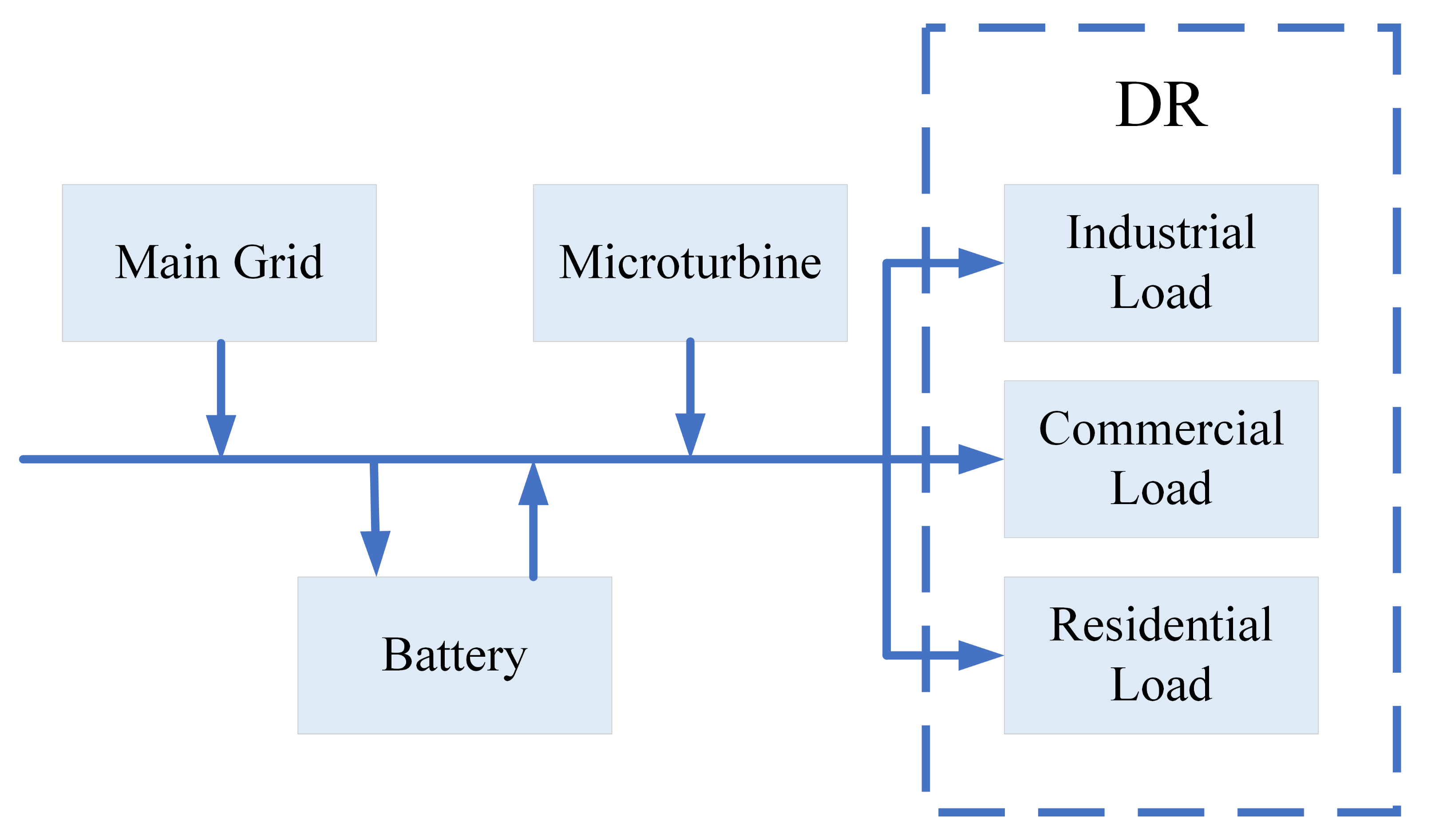
Figure 2.
The flowchart of the DE algorithm.

Figure 3.
The framework of the mixed differential evolution algorithm.

Figure 4.
ToUP during a day.

Figure 5.
Electric load during a day.

Figure 6.
Comparsion of algorithms in three dimensions.

Figure 7.
Local amplification.

Figure 8.
Comparsion of algorithms in 4 dimensions.

Figure 9.
Convergence graph of PCBSE in three scenarios.

Figure 10.
Cost at ToUP and IBRs.

Figure 11.
Power of each equipment at ToUP.

Figure 12.
Power of each equipment at IBRs electricity price.


Table 1.
Time-of-use pricing.
| Period Type | Period | Electricity Price (USD/(MW·h)) |
|---|---|---|
| Peak | 09.00–12.00 | 103.11 |
| 19.00–22.00 | ||
| Shoulder | 08.00–09.00 | 66.59 |
| 12.00–19.00 | ||
| 22.00–24.00 | ||
| Off-peak | 00.00–08.00 | 36.21 |
Table 2.
The parameters of the battery.
| Parameters | Values |
|---|---|
| maintenance price ($/(MW·h)) | 13.08 |
| depreciation price ($/(MW·h)) | 31.44 |
| minimum power (MW) | −0.1 |
| maximum power (MW) | 0.1 |
Table 3.
The scenarios studied in the experiments.
| Scenario | Period | Type of Electricity Price | Load (MW) |
|---|---|---|---|
| 1 | 00.00–08.00 | ToUP | 1.8 |
| 2 | 12.00–19.00 | ToUP | 2 |
| 3 | 12.00–19.00 | IBRs | 2 |
Table 4.
The design of the algorithms.
| Number | Name | Mutation | Crossover | Selection | Time Complexity |
|---|---|---|---|---|---|
| 1 | PBS | DE/pbest/1 | bin | SR | |
| 2 | PBE | DE/pbest/1 | bin | EC | |
| 3 | CBS | DE/current -to-pbest/1 | bin | SR | |
| 4 | CBE | DE/current -to-pbest/1 | bin | EC | |
| 5 | RCBSE | DE/rand/1 + DE/current -to-best/1 | bin | SR + EC | |
| 6 | PCBSE | DE/pbest/1 + DE/current -to-pbest/1 | bin | SR + EC | |
| 7 | PEE | DE/pbest/1 | exp | EC | |
| 8 | PCESE | DE/pbest/1 + DE/current -to-pbest/1 | exp | SR + EC |
Table 5.
The comparison of the algorithms.
| Algorithm | Scenario 1 ($/h) | Scenario 2 ($/h) | Scenario 3 ($/h) | Distance ($/h) | Rank |
|---|---|---|---|---|---|
| PBS | 297.0841 | 350.9401 | 315.3181 | 15.8529 | 6 |
| PBE | 297.7589 | 350.6436 | 322.9923 | 8.3722 | 2 |
| CBS | 296.5217 | 350.6883 | 314.4773 | 16.6914 | 7 |
| CBE | 297.2674 | 350.2056 | 319.1222 | 12.1702 | 4 |
| RCBSE | 296.5088 | 353.0914 | 316.4333 | 14.7180 | 5 |
| PCBSE | 296.3159 | 352.5341 | 325.1002 | 6.0320 | 1 |
| PEE | 298.8343 | 349.2507 | 306.3789 | 25.0215 | 8 |
| PCESE | 296.8377 | 348.3407 | 321.7752 | 10.0592 | 3 |
Table 6.
Wilcoxon Signed Rank Test.
| Sample | PBE | Distance | PCBSE | Distance | Difference | Rank |
|---|---|---|---|---|---|---|
| 1 | 320.8570 | 10.2549 | 326.2325 | 4.8794 | 5.3754 | 4 |
| 2 | 319.1282 | 11.9837 | 333.2710 | 2.1591 | 9.8246 | 6 |
| 3 | 318.8662 | 12.2457 | 330.5337 | 0.5782 | 11.6674 | 7 |
| 4 | 314.2184 | 16.8935 | 328.6028 | 2.5091 | 14.3844 | 8 |
| 5 | 331.7966 | 0.6847 | 323.2957 | 7.8162 | −7.1315 | 5 |
| 6 | 306.2662 | 24.8457 | 335.3584 | 4.2465 | 20.5992 | 10 |
| 7 | 328.3875 | 2.7244 | 331.4038 | 0.2919 | 2.4326 | 2 |
| 8 | 325.4941 | 5.6178 | 328.5918 | 2.5201 | 3.0977 | 3 |
| 9 | 308.4960 | 22.6159 | 324.2066 | 6.9053 | 15.7106 | 9 |
| 10 | 322.5186 | 8.5933 | 321.6220 | 9.4899 | −0.8966 | 1 |
Table 7.
Stability and Reliability Study.
| Parameters | Values | Results |
|---|---|---|
| F0 | 0.3 | 352.0413 |
| 0.5 | 352.0413 | |
| 0.7 | 352.0452 | |
| np | 50 | 352.0413 |
| 100 | 352.0413 | |
| 150 | 352.0414 | |
| CR | 0.8 | 352.0415 |
| 0.9 | 352.0413 | |
| 1 | 352.0413 |
Disclaimer/Publisher’s Note: The statements, opinions and data contained in all publications are solely those of the individual author(s) and contributor(s) and not of MDPI and/or the editor(s). MDPI and/or the editor(s) disclaim responsibility for any injury to people or property resulting from any ideas, methods, instructions or products referred to in the content. |
© 2023 by the authors. Licensee MDPI, Basel, Switzerland. This article is an open access article distributed under the terms and conditions of the Creative Commons Attribution (CC BY) license (https://creativecommons.org/licenses/by/4.0/).
Share and Cite
MDPI and ACS Style
Zhang, L.; Tang, R. Dispatch for a Continuous-Time Microgrid Based on a Modified Differential Evolution Algorithm. Mathematics 2023, 11, 271. https://doi.org/10.3390/math11020271
AMA Style
Zhang L, Tang R. Dispatch for a Continuous-Time Microgrid Based on a Modified Differential Evolution Algorithm. Mathematics. 2023; 11(2):271. https://doi.org/10.3390/math11020271
Chicago/Turabian StyleZhang, Lei, and Rui Tang. 2023. "Dispatch for a Continuous-Time Microgrid Based on a Modified Differential Evolution Algorithm" Mathematics 11, no. 2: 271. https://doi.org/10.3390/math11020271
Note that from the first issue of 2016, this journal uses article numbers instead of page numbers. See further details here.