Eulerian–Eulerian RSTM-PDF Modeling of Turbulent Particulate Flow

Abstract

A novel 3D computational model was developed for the turbulent particulate two-phase flow simulation in the rectangular channel. The model is based on the Eulerian approach applied to 3D Reynolds-averaged Navier–Stokes modeling and statistical Probability Distribution Function method. The uniqueness of the method lies in the direct calculation of normal and transverse components of the Reynolds stresses for both gas and particles. Two cases were examined: a conventional channel flow and grid-generated turbulence flow. The obtained numerical results have been verified and validated by the experimental data, received from the turbulent particle dispersion test. The computed values of the particles’ turbulent dispersion and the maximum value of the particulate concentration distribution show good agreement with the experimental results. The examples are ranged from coal and other bulk material pneumatic transport, vertical fluidized beds, coal gasifiers, and chemical reactors.

1. Introduction

Turbulent channel particulate flows are relevant to various branches of industry. Examples range from coal and other bulk material pneumatic transport, vertical fluidized beds, coal gasifiers, and chemical reactors. The complexity of the physical phenomena modeling is explained by particle–turbulence and particle–particle interactions, wall interactions and deposition, gravitational and viscous drag forces, particle rotation and lift forces, and turbulent dispersion. It becomes much more complex with the additional inclusion of coupling mechanisms and inter-particle collisions. The 2D simulation cannot comprehensively catch the whole process; therefore, only the 3D simulation model can explain the process in detail. In the two-fluid model, both the gas and the particles are considered as two coexisting phases that span the entire flow domain, each flowing with its mass fraction. In the case of polydispersed solid mixtures, each solid fraction is characterized by its mass fraction. Momentum interactions between the two phases are characterized by the drag and lift forces, which appear as a source term in the numerical computations.

There are several successful particulate flow simulation techniques in the practice of Computational Fluid Dynamics (CFD). Phenomenological models for particulate flows in pipes have been developed in the past [1,2]. The turbulence plays an important role in such flows, where the particles are often controlling the carrier fluid turbulence structure [3,4,5,6]. One of the most common ways of modeling the turbulent particulate flow is the Reynolds-averaged Navier–Stokes (RANS) approach. With this approach, the phase-averaged conservation of mass and momentum equations are solved by coupling with a statistical model proposed by Zaichik [7,8,9,10,11]. However, the method is using the k-ε model and does not describe flows in complex geometries with precise accuracy, for example, in rectangular or square channels. These flows are considerably anisotropic for the components of the turbulence energy, which are vividly expressed near the channel walls and corners and notable for the secondary flows. In addition, the presence of particles aggravates anisotropy. Such flows are studied with the Reynolds Stresses Turbulence Model (RSTM) approach, which is based on describing the transport equations for all components of the Reynolds stress tensor and the turbulence dissipation rate. The RSTM approach allows for completely analyzing the influence of particles on the longitudinal, radial, and azimuthal components of the turbulence kinetic energy, including possible modifications of the cross-correlation velocity moments. Several studies based on the RSTM approach produced accurate results and demonstrated the ability of the method to simulate complex flows [12,13], as well as turbulent transonic [14], supersonic [15], and viscoelastic flows [16]. Taulbee et al. [12] used the RSTM approach to calculate the particle-laden shear flow by applying the direct numerical simulation (DNS) and the small Reynolds number was used in their simulation, Re = 952. The recent investigation of particle-laden flows by numerical means with the DNS method is presented in [17]. The authors established correlations in interfacial terms in the dissipation equation and Reynolds stresses equations of carrier fluid with the DNS resolved method with a Reynolds number below 250. This is barely applicable to the real turbulent flows, characterized by considerably higher Reynolds numbers. The Probability Distribution Function (PDF) approach is widely applied for numerical modeling of the particulate flows. The PDF method [18,19] offers reasonable formalism in governing mass and momentum equations. It uses more complete differential transport equations for the particulate suspension. The mesh is defined for each particle–velocity variation and all process mechanisms of particle–turbulence and particle–particle interactions. The transport equations are written in terms of various velocity correlations, which may consider either the fluid turbulence augmentation or attenuation caused by the presence of the particles [10,11,20,21,22]. Zaichik [7] introduced a new PDF approach and they used Boussinesq approximation for the particulate motion equations and algebraic expressions for particle-phase turbulent viscosity and diffusion coefficients. This approach was also used by Kartushinsky et al. [23], who applied the RSTM closures to the carrier phase and, simultaneously, the closures from the Boussinesq hypothesis for the particulate phase. Mukin and Zaichik [7] proposed a nonlinear algebraic Reynolds stress model based on the PDF approach to solve a gas flow loaded by small heavy particles. The equations were written for each Reynolds stress component and reduced to their general form in terms of the turbulence energy and turbulence dissipation rate. This way considered additional impact from the particulate phase. However, this model does not solve the differential transport equations and requires use of an additional model for the solution. There are different approaches and numerical models that describe the mutual effect of gas turbulence and particles. The k-ε models are considered turbulence attenuation only by the additional terms of the turbulence kinetic energy and its dissipation rate equations [3,24,25,26,27]. The simulation of the inter-particle collisions in the case of the turbulent dense particulate flows are considered in [28]. However, the model becomes over-complicated and takes a huge amount of computational time, especially for a long channel case. Thus, there is room for improvement. As opposed to the k-ε models, Schwarzkopf, Crowe and Dutta [29] and Crowe [30] considered both the turbulence augmentation caused by the velocity slip between gas and particles and the turbulence attenuation due to the change of the turbulence macroscale, which occurred in the particulate flow as compared to the unladen flow. The flow of mass loading and the Stokes number play a crucial role in modeling. The given approach was successfully tested for various pipe and channel particulate flows. Later, a statistical PDF model was elaborated on, covering the solution for each particle Reynolds stress component [9] and making a solution much easier. The mutual effect of particles and flow turbulence has been a subject of numerous theoretical studies for several decades. These studies have reported the influence of gas turbulence on particles, called one-way coupling. The influence of the particles on the turbulence of a carrier gas flow is called two-way coupling. Four-way coupling will occur in the case of high flow mass loading. The impact of particles on gas turbulence consists of turbulence attenuation or augmentation, which in turn depend on the relationship between the gas and particle parameters. Stojanovic et al. [31] and Geiss et al. [32] experimentally investigated the effect of grid-generated turbulence modification using solid particles of two sizes: 120 and 480 microns. Their model showed that smaller-size particles have attenuated turbulence, whereas larger-size particles have additionally generated turbulence. Hussainov et al. [33] have shown that for up to 0.07 (kg dust/kg air) mass loading, the 700 micron glass particles were attenuated turbulence in the initial period of turbulence decay. The experimental test had two Reynolds numbers (ReM = 3040 and 6300) determined for two grid sizes (4.8 and 10 mm). Additional turbulence generation by the same-size particles was noticed in the case of twice-increased mass loading [34]. Von Karman [35] studied the homogeneous turbulence configuration. Here, the interactions between the turbulence and mean flow are sustained by a mean shear constant. In one of the earliest experiments, Champagne et al. [36] showed that even when the turbulent intensities and stresses are both effectively homogeneous, the turbulent length–scale grows downstream. Subsequently, Harris et al. [37] found that for a given sufficient time of the flow development, the turbulence intensities are also monotonically increasing downstream. Later, Ahmed and Elghobashi [38] showed that the fluctuations of the longitudinal velocity component grow monotonically downstream, whereas the fluctuations of two other velocity components remain constant. New two-phase particulate flow computational model development is the main objective of this paper. Additionally, the simulation should track the particles’ influence on the carrier flow and compute the carrier flow turbulence. Finally, the model should apply to the high Reynolds numbers and track the particles’ influence on the carrier fluid flow. For this reason, the paper is presented as follows. The Numerical Method and Assumptions section is explaining the new model equations with applicability constraints. Then, the Results and Discussions section introduces an application of a new elaborated 3D model for three types of turbulent horizontal channel particulate flows:(1) grid-generated turbulence, (2) classical channel turbulence, and (3) shear flow. The new model allows direct calculation of the normal and shear components of the Reynolds stresses for both the gas flow and particles. The present numerical simulation extends the model to apply to Reynolds numbers up to 70,000. The numerical calculation results have been validated with a set of experimental data presented in this paper.

2. Numerical Method and Assumptions

2.1. Scale of the Investigation

This article presents a theoretical three-dimensional flow model with a dilute mixture of particles moving in a carrier gas. The particulate phase was treated as a continuous medium, where the inter-particle collisions were ignored. This work examined two main cases: (1) grid-generated turbulence flow and (2) usual turbulent channel flow. For comparison purposes, the plots have a shear flow along the y-direction. The numerical results were borrowed from [20]. The simulation model used a Cartesian coordinate system, where x is the streamwise coordinate, y is the transverse coordinate, and z is the bottom–normal (azimuthal) coordinate; u, v, and w are the associated velocity components, respectively. Figure 1 shows the directions of the channel flow of the 2 m long and 0.4 × 0.2 m² cross-sectional area.

2.2. Computational Method

The control volume method was applied to solve three-dimensional partial differential equations for the particle-loaded flow. The governing equations were solved using the implicit lower and upper (ILU) matrix decomposition method with the flux-blending differed-correction and upwind-differencing schemes [39,40]. The calculations were performed in the dimensional form for all flow conditions. The simulation mesh contained 1,120,000 control volumes.

2.3. Governing Equations for the Carrier Fluid

Continuity equation:

$$\frac{\partial \rho }{\partial t}+\frac{\partial \rho u_i}{\partial x_i}=0$$

(1)

Momentum equation:

$$\frac{\partial u_i}{\partial t}+u_k\frac{\partial u_i}{\partial x_k}=\frac{\partial }{\partial x_i}\left(\nu \frac{\partial u_i}{\partial x_j}\right)-\frac{\partial \overline{u_i^{\prime }{u}_j^{\prime }}}{\partial x_j}-\frac{\partial p}{\rho \partial x_i}-\alpha \frac{\left(u_i-u_{si}\right)}{{\tau }_p}$$

(2)

Reynolds stresses transport equations:

$$\begin{array}{c}\frac{\partial \overline{u_i^{\prime }{u}_j^{\prime }}}{\partial t}+u_k\frac{\partial \overline{u_i^{\prime }{u}_j^{\prime }}}{\partial x_k}=\nu \frac{\partial \overline{u_i^{\prime }{u}_j^{\prime }}}{{\partial }_k}+C_s\left(\overline{u_i^{\prime }{u}_l^{\prime }}\frac{\partial \overline{u_j^{\prime }{u}_k^{\prime }}}{\partial x_l}+\overline{u_j^{\prime }{u}_l^{\prime }}\frac{\partial \overline{u_i^{\prime }{u}_k^{\prime }}}{\partial x_l}+\overline{u_k^{\prime }{u}_l^{\prime }}\frac{\partial \overline{u_i^{\prime }{u}_j^{\prime }}}{\partial x_l}\right)\\ +P_{ij}+R_{ij}-\frac{2}{3}\epsilon {\delta }_{ij}\end{array}$$

(3)

Dissipation transport equation:

$$\frac{\partial \epsilon }{\partial t}+u_k\frac{\partial \epsilon }{\partial x_k}=\frac{\partial }{\partial x_i}\left(\nu +C_s\frac{k}{\epsilon }\overline{u_i^{\prime }{u}_j^{\prime }}\frac{\partial \epsilon }{\partial x_j}\right)+C_{\epsilon 1}\frac{P\epsilon }{k}-C_{\epsilon 2}\frac{{\epsilon }^2}{k}$$

(4)

The above-written RSTM equations were given from the LRR (Laouner, Rodi, Reece)turbulence model [41].

2.4. Governing Equations for the Particulate Phase

The particle mass conservation equation [20]:

$$\frac{\partial \alpha }{\partial t}+\frac{\partial \alpha u_{sk}}{\partial x_k}=-\frac{\partial \overline{{\alpha }^{\prime }{u}_{sk}^{\prime }}}{\partial x_k}$$

(5)

The momentum equation of the dispersed phase:

$$\frac{\partial u_{si}}{\partial t}+u_{sk}\frac{\partial u_{sk}}{\partial x_k}=-\frac{\partial \overline{u_{si}^{\prime }{u}_{sk}^{\prime }}}{\partial x_k}+\frac{u_i-u_{si}}{{\tau }_p}+F_i-\frac{D_{pki}}{{\tau }_p}\frac{\partial \alpha }{\partial x_k}$$

(6)

In the above equations, u, v, and w are the axial-, transverse-, and span-wise time-averaged velocity components of the gas, respectively; $u_s$, $v_s$, and $w_s$ are the axial-, transverse-, and span-wise time-averaged velocity components of the particulate phase, respectively; $\rho$ is the material density of gas; ${\rho }_p$ is the material density of the particles; α is the particle concentration; $g_x$ and $g_y$ are the components of the gravitational acceleration in the x and y directions; and ${C^{\prime }}_D$ is the friction coefficient based on the relative velocity between the phases. The turbulent dispersion coefficient, $D_s$, has been calculated using a PDF model calculating closures for the transport coefficients of the particulate phase. The momentum equation of the dispersed phase in the Cartesian coordinates is given in Appendix A Equations (A1)–(A4) and Reynolds stresses’ components of the dispersed phase are also given in Appendix A Equations (A5)–(A10).

The PDF approach was used to write the second-order moment equations of the fluctuating velocity (turbulent stresses) of the particulate phase. The equations describe the convective and diffusive transfer, the generation of particle velocity fluctuations due to the velocity gradients, the generation of fluctuations resulting from the entrainment of particles into the fluctuating motion of the carrier gas flow, and the dissipation of turbulent stresses in the particulate phase caused by interfacial forces. The equation for the x-component of the Reynolds stress is as follows:

The equations for the particle-phase Reynolds stresses:

$$\begin{array}{l}\frac{\partial \overline{u_{si}^{\prime }{u}_{sj}^{\prime }}}{\partial t}+u_{sk}\frac{\partial \overline{u_{si}^{\prime }{u}_{sj}^{\prime }}}{\partial x_k}-\frac{1}{3\alpha }\frac{\partial }{\partial x_k}\alpha \left(D_{pin}\frac{\partial \overline{u_{sj}^{\prime }{u}_{sk}^{\prime }}}{\partial x_n}+D_{pjn}\frac{\partial \overline{u_{si}^{\prime }{u}_{sk}^{\prime }}}{\partial x_n}+D_{pkn}\frac{\partial \overline{u_{si}^{\prime }{u}_{sj}^{\prime }}}{\partial x_n}\right)\\ =-\left(\overline{u_{si}^{\prime }{u}_{sk}^{\prime }}+{\mu }_{ik}\right)\frac{\partial u_{sj}}{\partial x_k}-\left(\overline{u_{sj}^{\prime }{u}_{sk}^{\prime }}+{\mu }_{jk}\right)\frac{\partial u_{si}}{\partial x_k}+{\lambda }_{ij}{\lambda }_{ji}-\frac{2}{{\tau }_p}\overline{u_{si}^{\prime }{u}_{sj}^{\prime }}\end{array}$$

(7)

where the tensor of the turbulent diffusion of particles is defined as:

$$D_{pij}={\tau }_p\left(\overline{u_{si}^{\prime }{u}_{sj}^{\prime }}+{\mu }_{ij}\right)={\tau }_p\left(\overline{u_{si}^{\prime }{u}_{sj}^{\prime }}+\overline{u_i^{\prime }{u}_k^{\prime }}{g}_{kj}\right)+O\left({\tau }_p^2\right),$$

$${\lambda }_{ij}=\overline{u_i^{\prime }{u}_k^{\prime }}\left(\frac{f_{ukj}}{{\tau }_p}+l_{ukn}\frac{\partial u_j}{\partial x_n}+{\tau }_p{m}_{ukl}\frac{\partial u_n}{\partial x_l}\frac{\partial u_j}{\partial x_n}\right),{\mu }_{ij}=\overline{u_i^{\prime }{u}_k^{\prime }}\left(g_{ukj}+{\tau }_p{h}_{ukn}\frac{\partial u_j}{\partial x_n}\right)$$

The values ${\lambda }_{ij}$ and ${\mu }_{ij}$ are integrals having second correlation moments of the carrier fluid along the trajectory of the particles.

The coefficients $g_u^l$, $g_u^n$, and $g_u^k$ characterize the entrainment of particles into the fluctuating motion of the flow along the x, y, and z directions, respectively. The Fick’s approach has been used for the closure of the particle mass concentration fluctuation correlations and particle velocity components in three directions.

2.5. Boundary Conditions

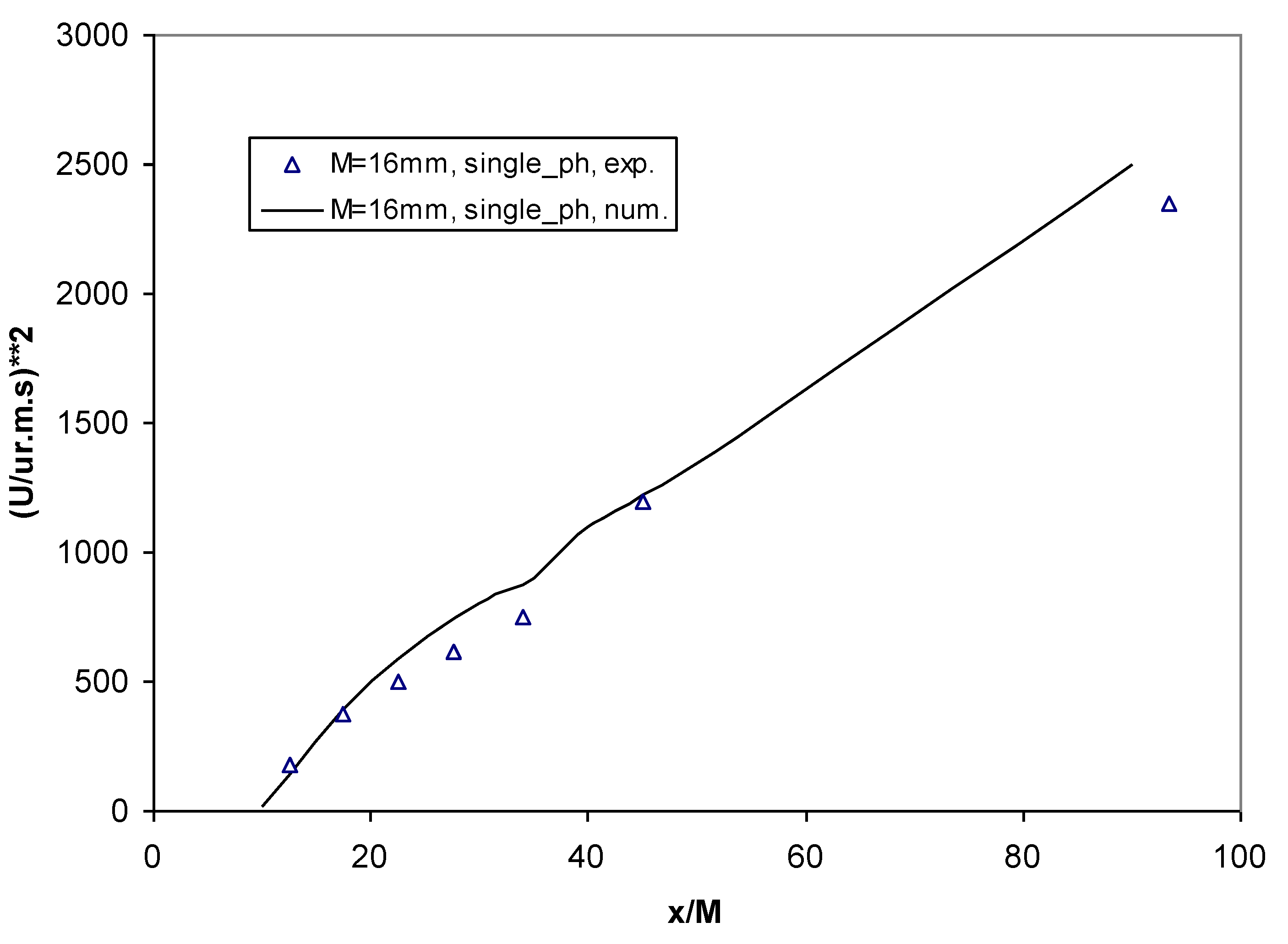
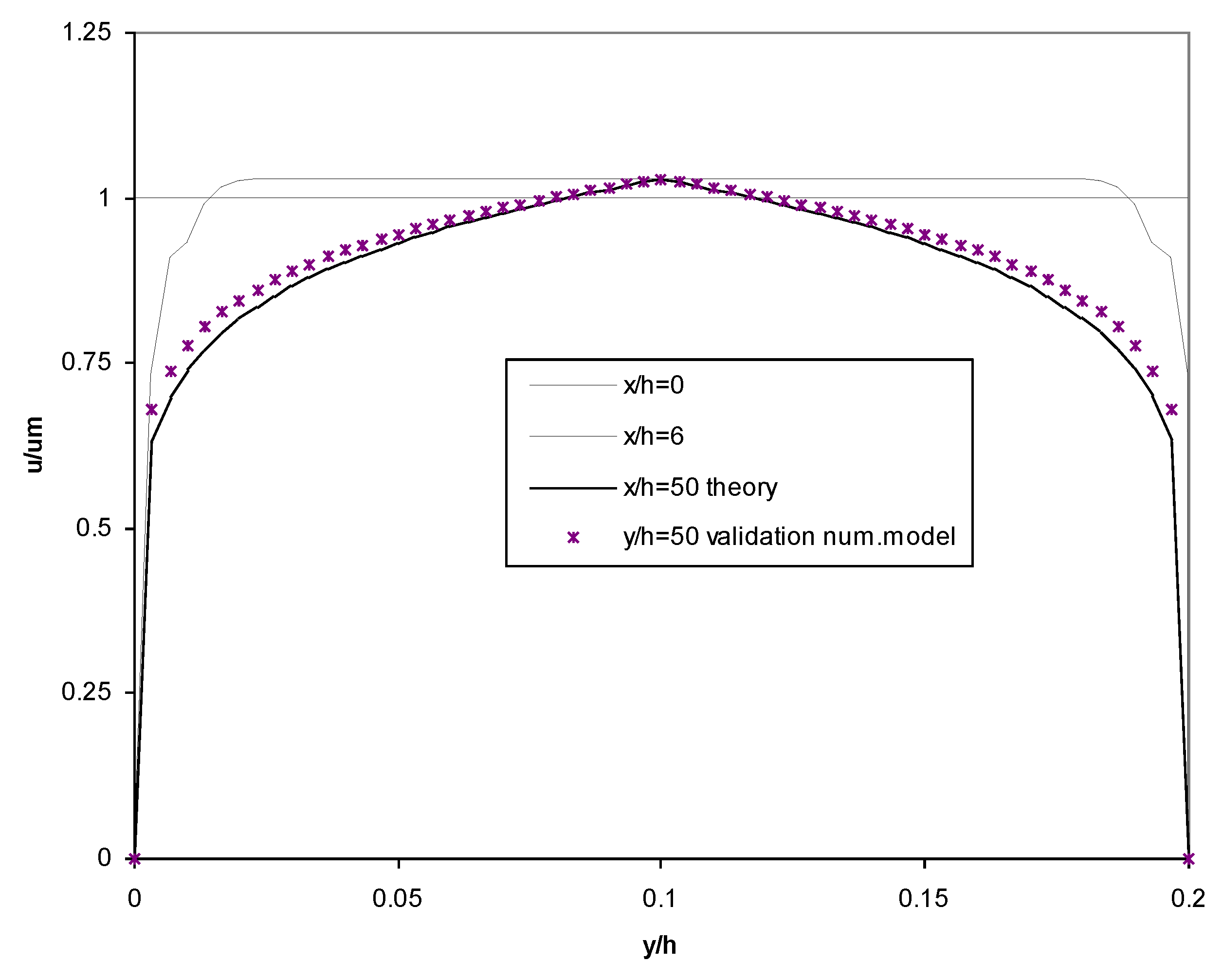
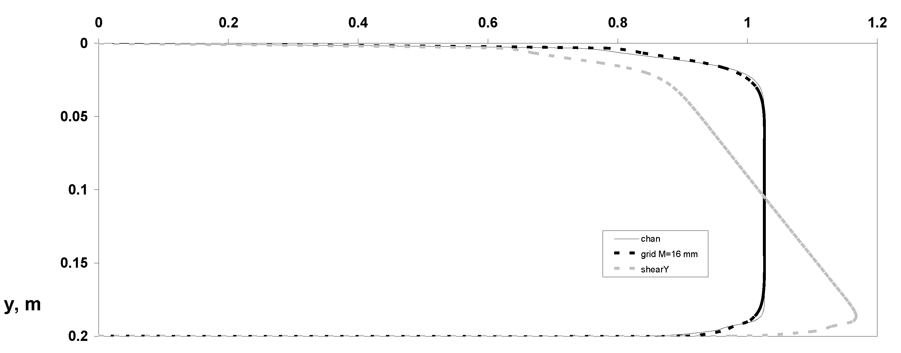
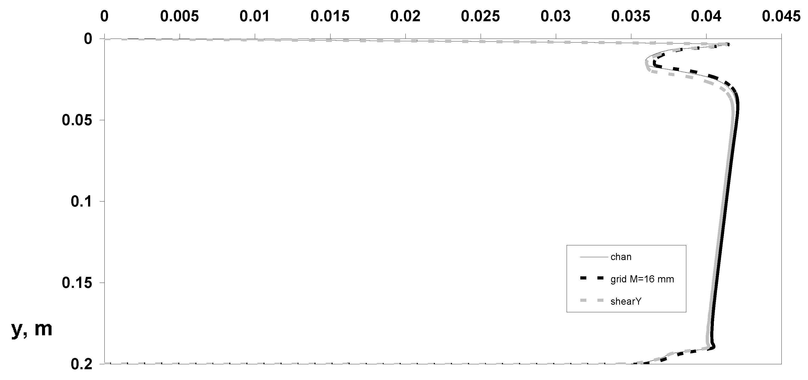
The wall boundary conditions for the gas flow are based on the control volume method, developed by Perić and Scheuerer [39] and Fertziger and Perić [40]. The boundary conditions for the particulate phase at the channel walls were set according to Zaichik [10]. At the exit of the channel, the boundary conditions for the gas and particulate phase are as follows:

$$\frac{\partial u_s}{\partial x}=\frac{\partial v_s}{\partial x}=\frac{\partial w_s}{\partial x}=\frac{\partial \alpha }{\partial x}=\frac{\partial \overline{{u_s^{\prime }}^2}}{\partial x}=\frac{\partial \overline{{v_s^{\prime }}^2}}{\partial x}=\frac{\partial \overline{{w_s^{\prime }}^2}}{\partial x}=\frac{\partial \overline{u_s^{\prime }{v}_s^{\prime }}}{\partial x}=\frac{\partial \overline{u_s^{\prime }{w}_s^{\prime }}}{\partial x}=\frac{\partial \overline{v_s^{\prime }{w}_s^{\prime }}}{\partial x}=0$$

(8)

Inlet boundary conditions are set as the following:

$$u_s=u,v_s=w_s=\overline{{v_s^{\prime }}^2}=\overline{{w_s^{\prime }}^2}=\overline{v_s{w}_s}=0,\overline{{u_s^{\prime }}^2}=\overline{{u^{\prime }}^2}$$

(9)

$$\{\begin{array}{cc}\alpha =\kappa & -\Delta y\le y\le \Delta y;-\Delta z\le z\le \Delta z\\ \alpha ={10}^{-6}\kappa & -y<-\Delta y,y>\Delta y;-z<-\Delta z,z>\Delta z\end{array}$$

(10)

where the parameter $\kappa$ is defined as particle mass loading. It can be roughly estimated by knowing the number of particles per volume unit. From the experimental data [42], 17 particles per 1 cm³ were experimentally estimated. With application to the relationship ${\rho }_p\beta =\rho \alpha$, where $\beta$ is the particle volume fraction, one can easily compute particle mass loading as 0.04.

The normal Reynolds stress components are defined as follows:

$$\overline{{u^{\prime }}^2}=u^2\times 0.0016$$

(11)

$$\overline{{v^{\prime }}^2}=\overline{{w^{\prime }}^2}=\overline{{u^{\prime }}^2}$$

(12)

For the turbulence grid flow, the normal Reynolds stresses’ components are defined as follows:

$$\overline{{u^{\prime }}^2}=u^2\times 0.0046,\overline{{v^{\prime }}^2}=\overline{{w^{\prime }}^2}=\overline{{u^{\prime }}^2}$$

(13)

2.6. Validation

The numerical simulation results were validated with the experimental data coming from [20]. The testing facility was similar to the one reported by Philips et al. [43] and allowed for observing the shear–particulate flow with flat plates with a variable pitch. The test section was 2 m long with a 0.4 × 0.2 m² cross-sectional area channel. The high-speed camera recorded particle trajectories to measure the particle dispersion. The camera translated and focused on several areas along the length of the test section. Then, with electronically processing the video frames, the average dispersion of the particles was determined. The simulation results matched with experimental data by a 0.5% error, which shows a good agreement. The 16 mm mesh size was used to generate the mesh generated turbulence flow. As can be seen in Figure 2, the experimental data and numerical results are in good agreement [21].

Figure 3 shows the axial component of the average velocity of the carrier fluid (gas), numerically calculated in the 3D square channel with the side size of 0.2 mm and mean velocity of 9.5 m/s. Here, velocity profiles are dimensionless related to average velocity at the channel axis (Um). It is presented along the whole width of the height of the channel from one wall to another wall using the RSTM approach. It is seen that modeling adequately illustrates the profile of velocity at the steady state flow (y/h = 50, dashed crosses curve) with satisfactory behavior versus classical turbulent channel flow velocity distribution (solid line “theory”, Figure 3). However, in the given research, we focus on results obtained not far from the inlet cross-section of the particle-laden flow (see broken line merked by x/h = 6). Here, “theory” means the typical velocity profile is taken from a classical book [44].

3. Results and Discussions

Three types of flow structures were examined: the conventional flow or typical channel flow, grid-generated turbulence flow, and shear flow directed towards the gravitation direction [20,21]. The plots present the following:

-

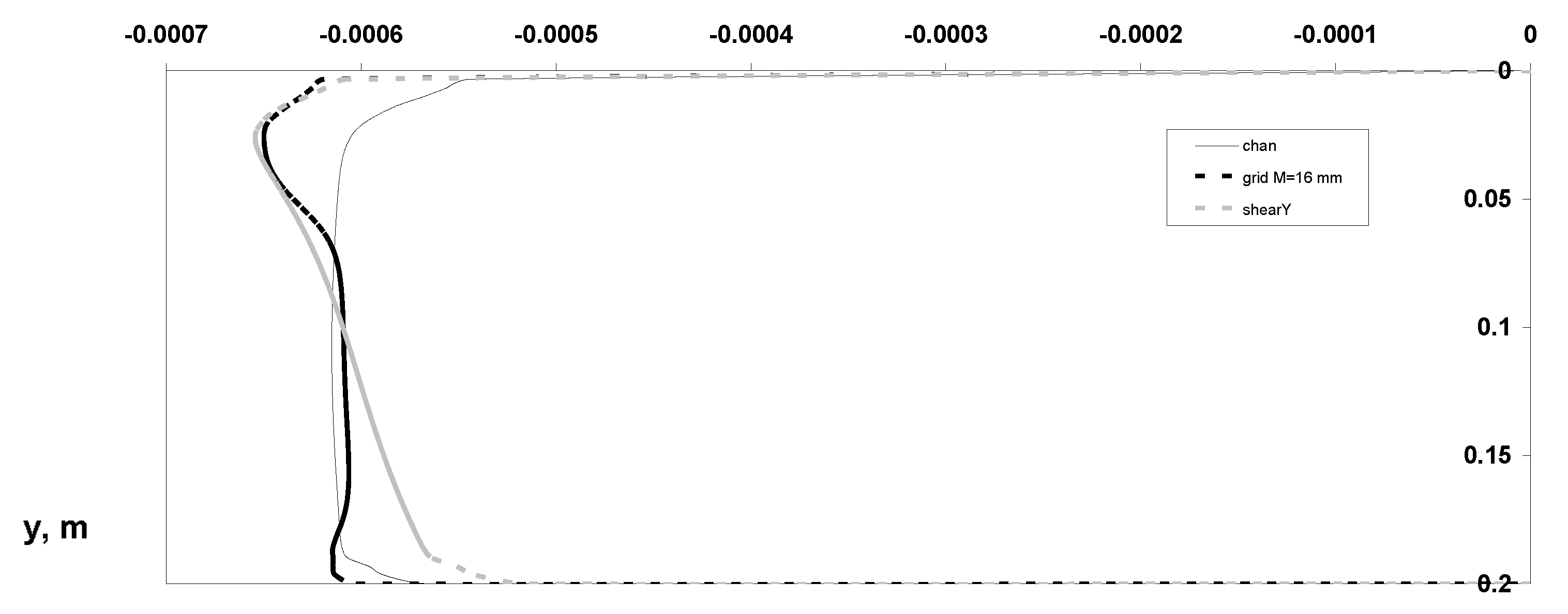
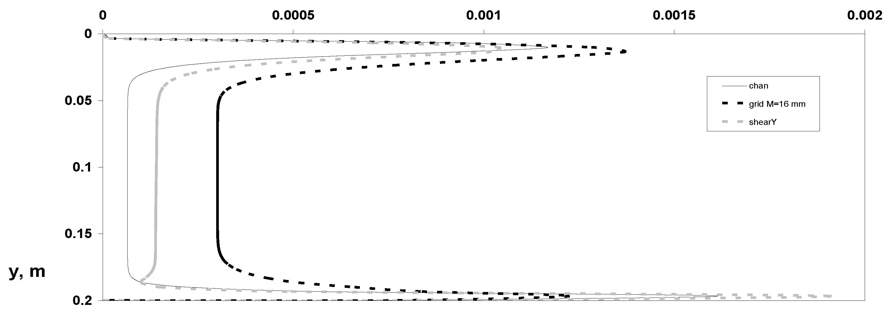
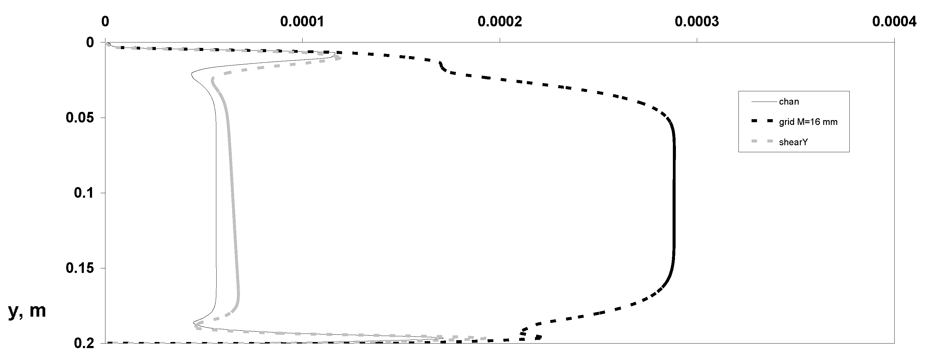
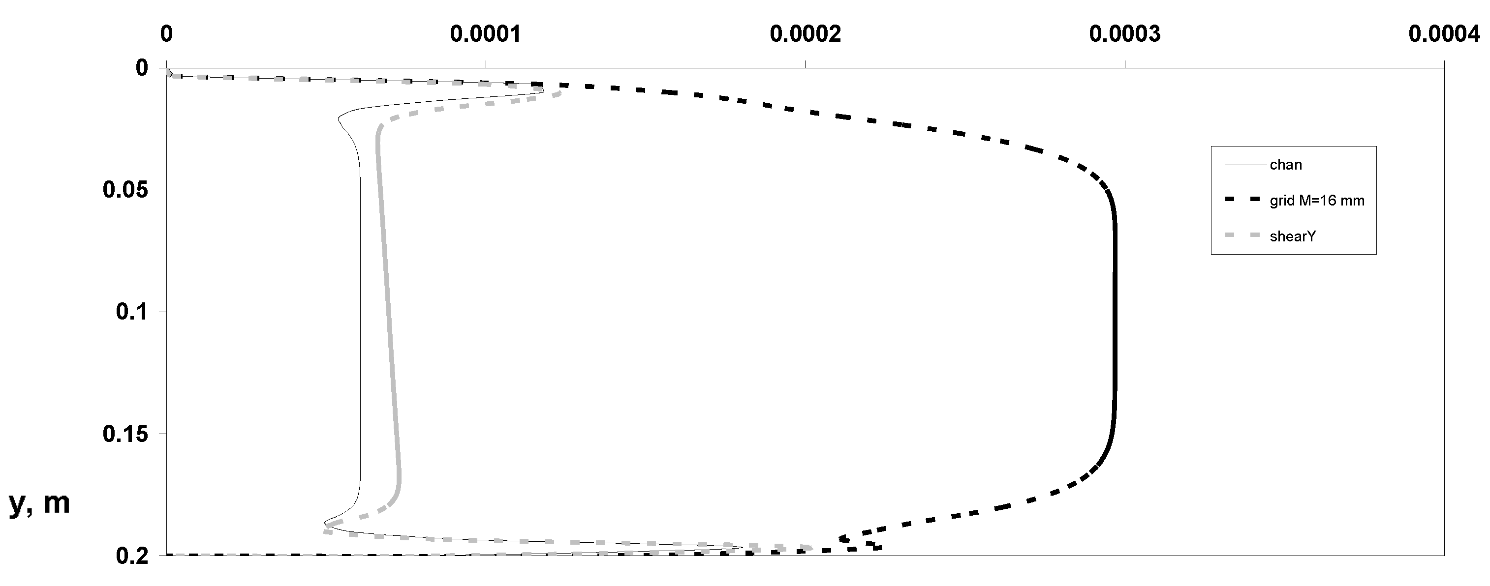
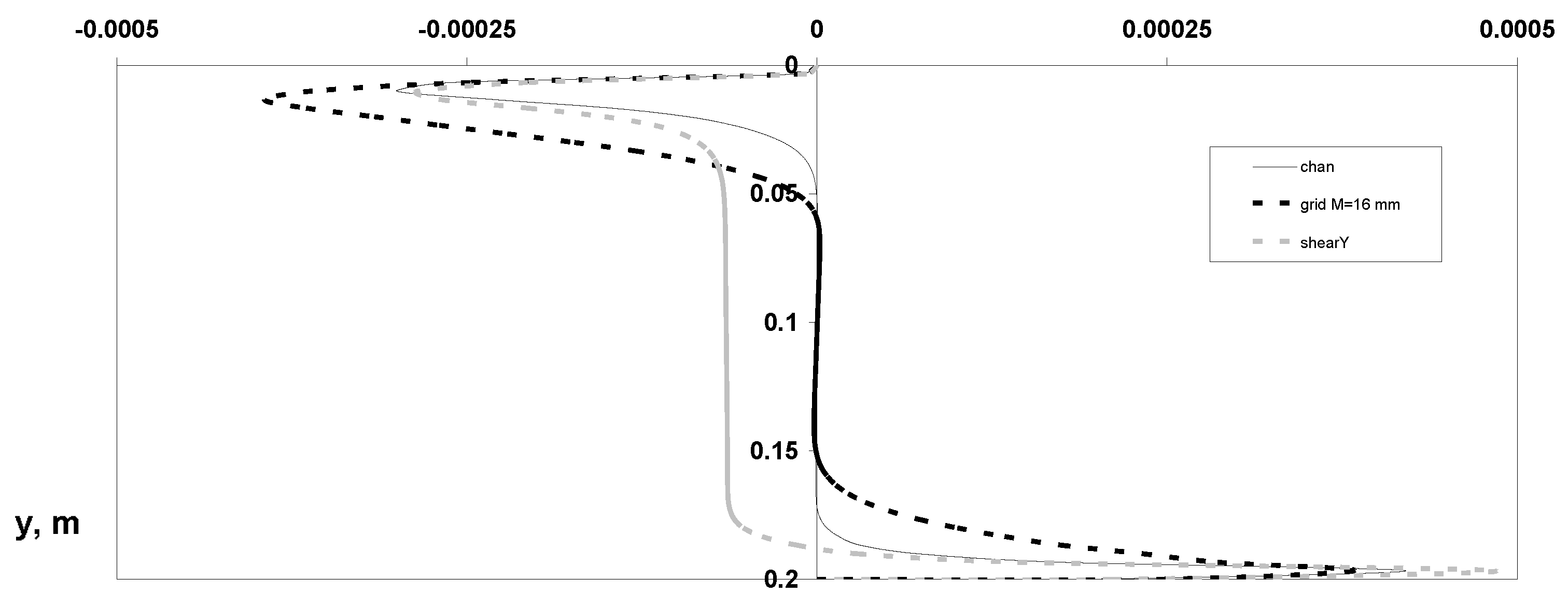
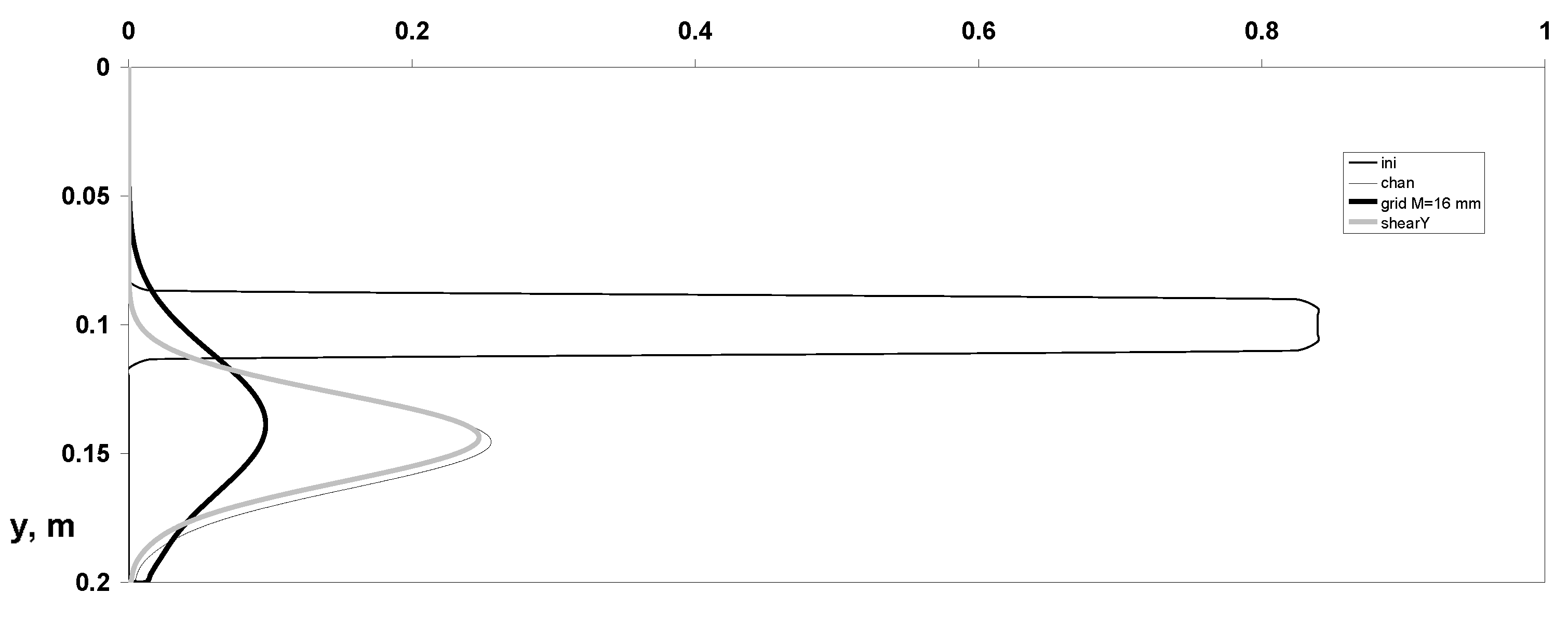
Distributions of dynamic parameters of the particulate phase for averaged various velocity components;

-

Reynolds stresses’ components;

-

Particle mass concentration, omitting distributions of parameters of the carrier gas-phase flow for its simplicity.

Figure 4 shows two cases of 3D turbulent transverse distributions of particles’ axial velocity in the conventional flow, the grid-generated turbulence flow. Additionally, the shear flow with the linear distribution of the gas-phase axial velocity component was added to the plot. The velocity profiles show a similar character to the grid products and channel flow. The shear flow has a maximum value shifted down to the bottom of the channel. This may happen due to particles’ involvement in the flow motion in the shear case.

The next profiles are observed for the distribution of the averaged transverse velocity components of the particulate phase along the transverse direction (Figure 5) for three considered flow structures. As noticed, the transverse velocity component of the particulate phase slowly decreases towards the bottom channel wall. It occurred due to the balance between viscous drag force and gravitation force. The small wiggles of velocity profiles near the top channel wall are due to the opposite direction towards gravitation of particle dispersion near the top wall. A high level of turbulence of the carrier gas–flow was observed at this location.

Figure 6 depicts the azimuthal velocity component distributions along the transverse direction. The plot shows the typical flat profile with a small velocity magnitude compared to its axial velocity component. It has occurred for the conventional and grid-generated turbulence types of flow. However, for the shear case, one may see the slight growth of this velocity component towards the bottom channel wall, which is probably a high value of the axial velocity at the bottom wall in a given case.

The normal axial Reynolds stress tensor component of the particulate phase is shown in Figure 7. It has maximum value spikes at the top and bottom walls of the channel. The shear flow of the normal Reynolds stress spike is higher at the bottom wall than at the top wall. The reason for this is a higher particulate axial velocity at the bottom versus the velocity component at the top channel wall.

Figure 8 and Figure 9 show the normal transverse and azimuthal Reynolds stress tensor components $\overline{{v_s^{\prime }}^2}$ and $\overline{{w_s^{″}}^2}$ that are similar to conventional and shear flow cases. Normally, the typical distribution of turbulent energy has a flat profile across the turbulent core with its maximum value near the walls. In contrast, the grid-generated turbulence flow has a kind of flat shape with almost the same magnitudes for all three normal components, $\overline{{u_s^{\prime }}^2}$, $\overline{{v_s^{\prime }}^2}$, and $\overline{{w_s^{″}}^2}$, in the turbulent core, which is also observed in Figure 7, Figure 8 and Figure 9, indicating turbulence isotropy in the grid-generating turbulence flow.

The particulate phase Reynolds shear stress $\overline{u_s^{\prime }{v}_s^{\prime }}$ is small. However, for conventional and grid-generated turbulence cases, it is finite at the same region in the turbulent core and has a higher value for the shear flow case. This behavior is defined by the non-uniform shape in Figure 10, with a linear increase of the particle’s axial velocity across the flow. It means that joined 3D RANS and PDF models accurately illustrate the fluid dynamic parameters in all three different flow structures and deliver reasonable results.

Figure 11 shows profiles of particles mass concentration across channel flow from the top to the bottom walls in the various cross-sections downward channel flow. The numerical results presented in the following paragraphs were computed for two cases: (1) at the source location (x = 0) and (2) at a longitudinal distance equal to x/h = 12.63 from the particle source. The notation “ini” in Figure 11 shows the initial distribution of the particles’ mass concentration. The turbulent dispersion of the 55 μm glass spherical particles was calculated with a flow mass loading of 10⁻⁶ kg glass/kg air. For this reason, the flows were considered diluted. One can see (Figure 11) that due to gravitation and turbulence dispersion phenomena the particles go down and are spread out downstream channel flow.

4. Conclusions

The 3D Reynolds stress turbulence model was developed based on the 3D RANS and statistical PDF approaches for the two-phase turbulent flow of solid particles in the rectangular channel. The numerical results of the model on the dispersion of the particles have been verified with experimental data. Two cases were discussed:

• Grid-generated turbulent flow;
• Channel turbulent flow.

The shear flow case results were borrowed from the earlier work and used for comparison purposes. Several results on the mean flow velocities, the turbulence variables, the Reynolds shear stress, and the particle concentration in the transverse- and span-wise directions are reported in this paper. The utilization of the same closure equations in the CFD model for both the carrier flow and the particulate phase is the main benefit and novelty of the method. There are several advantages to the model:the ability to direct simulation of the particle concentration and the ability to direct simulation of the particle influence on the carrier flow, including the turbulence of the carrier flow.

References

1. Pfeffer, R.; Rosetti, S.; Licklein, S. Analysis and Correlation of Heat Transfer Coefficient and Heat Transfer Data for Dilute Gas–Solid Suspensions; NASA ReportTND3603; 1966. Available online: https://ntrs.nasa.gov/api/citations/19660026357/downloads/19660026357.pdf (accessed on 6 June 2023).
2. Michaelides, E.E. A model for the flow of solid particles in gases. Int. J. Multiph. Flow 1984, 10, 61–75. [Google Scholar] [CrossRef]
3. Elghobashi, S.; Abou-Arab, T.W. A two-equation turbulence model for twophase flows. Phys. Fluids 1983, 26, 931–938. [Google Scholar] [CrossRef]
4. Yarin, L.P.; Hetsroni, G. Turbulence intensity in dilute two-phase flows, Parts I, II and III. Int. J. Multiph. Flow 1994, 20, 1–44. [Google Scholar] [CrossRef]
5. Yuan, Z.; Michaelides, E.E. Turbulence modulation in particulate flows—A theoretical approach. Int. J. Multiph. Flow 1992, 18, 779–791. [Google Scholar] [CrossRef]
6. Crowe, C.T.; Gillandt, I. Turbulence modulation of fluid-particle flows—A basic approach. In Proceedings of the Third International Conference on Multiphase Flows, Lyon, France, 8–12 June 1998. [Google Scholar]
7. Zaichik, L. A statistical model of particle transport and heat transfer in turbulent shear flows. Phys. Fluids 1999, 11, 1521–1534. [Google Scholar] [CrossRef]
8. Mukin, R.V.; Zaichik, L.I. Nonlinear algebraic Reynolds stress model for two-phase turbulent flows laden with small heavy particles. Int. J. Heat Fluid Flow 2012, 33, 81–91. [Google Scholar] [CrossRef]
9. Zaichik, L.I.; Alipchenkov, V.M. Statistical models for predicting particle dispersion and preferential concentration in turbulent flows. Int. J. Heat Fluid Flow 2005, 26, 416–430. [Google Scholar] [CrossRef]
10. Zaichik, L.I.; Vinberg, A.A. Modeling of particle dynamics and heat transfer in turbulent flows using equations for first and second moments of velocity and temperature fluctuations. In Proceedings of the 8th Symposium on Turbulent Shear Flows, Munich, Germany, 9–11 September 1991; Volume 1, pp. 10-2-1–10-2-6. [Google Scholar]
11. Zaichik, L.I.; Alipchenkov, V.M. Refinement of the probability density function model for preferential concentration of aerosol particles in isotropic turbulence. Phys. Fluids 2007, 19, 113308. [Google Scholar] [CrossRef]
12. Taulbee, D.B.; Mashayek, F.; Barré, C. Simulation and Reynolds stress modeling of particle-laden turbulent shear flows. Int. J. Heat Fluid Flow 1999, 20, 368–373. [Google Scholar] [CrossRef]
13. Gerolymos, G.A.; Vallet, I. Contribution to Single-Point-Closure Reynolds-Stress Modelling of Inhomogeneous Flows. In Proceedings of the ASME/JSME 2003 4th Joint Fluids Summer Engineering Conference, Honolulu, HI, USA, 6–10 July 2003; American Society of Mechanical Engineers Digital Collection: New York, NY, USA, 2003; pp. 1989–1994. [Google Scholar]
14. Kim, K.-Y.; Cho, C.-H. Performance of Reynolds stress turbulence closures in the calculation of three-dimensional transonic flows. In Proceedings of the ASME Fluids Engineering Division Summer Meeting ASME FEDSM, New Orleans, LA, USA, 29 May–1 June 2001. FEDSM2001-18239, CD-ROM. [Google Scholar]
15. Abouali, O.; Ahmadi, G.; Rabiee, A. Computational simulation of supersonic flow using Reynolds stress model. In Proceedings of the ASME Fluids Engineering Division Summer Meeting ASME FEDSM, Houston, TX, USA, 19–23 June 2005. FEDSM2005-77434, CD-ROM. [Google Scholar]
16. Leighton, R.; Walker, D.T.; Stephens, T.; Garwood, G. Reynolds stress modeling for drag reducing viscoelastic flows. In Proceedings of the 4th ASME/JSME Joint Fluids Summer Engineering Conference FEDSM, Honolulu, HI, USA, 6–10 June 2003. FEDSM2003-45655, CD-ROM. [Google Scholar]
17. Xia, Y.; Yu, Z.; Lin, Z.; Guo, Y. Imporved modeling of interface terms in the second- moment closure for particle-laden flows based on interface-resolved simulation data. J. Fluid Mech. 2022, 952, A25. [Google Scholar] [CrossRef]
18. Reeks, M.W. On a Kinetic Equation for the Transport of Particles in Turbulent flows. Phys. Fluids A Fluid Dyn. 1991, 3, 446–456. [Google Scholar] [CrossRef]
19. Reeks, M.W. On the Continuum Equations for Dispersed Particles in Nonuniform Flows. Phys. Fluids A Fluid Dyn. 1992, 4, 1290–1303. [Google Scholar] [CrossRef]
20. Lauk, P.; Kartushinsky, A.; Hussainov, M.; Polonsky, A.; Rudi, Ü.; Shcheglov, I.; Tisler, S.; Seegel, K.E. Two-Fluid RANS-RSTM-PDF Model for Turbulent Particulate Flows. In Numerical Simulation: From Brain Imaging to Turbulent Flows; IntechOpen: London, UK, 2016; pp. 339–363. [Google Scholar]
21. Kartushinsky, A.; Rudi, Y.; Stock, D.; Hussainov, M.; Shcheglov, I.; Tisler, S.; Shablinsky, A. Numerical simulation of grid-generating turbulent particulate flow by three-dimensional Reynolds stress. Proc. Est. Acad. Sci. 2013, 62, 161–174. [Google Scholar] [CrossRef]
22. Kartushinsky, A.; Tisler, S.; Oliveira, J.L.G.; van der Geld, C.W.M. Eulerian-Elerian modeling of particle-laden two-phase flows. Powder Techol. 2016, 301, 999–1007. [Google Scholar] [CrossRef]
23. Kartushinsky, A.; Rudi, Y.; Hussainov, M.; Shcheglov, I.; Tisler, S.; Krupenski, I.; Stock, D. RSTM numerical simulation of channel particulate flow with rough wall. In Computational and Numerical Simulations; InTech: Rijeka, Croatia, 2014; pp. 41–63. [Google Scholar]
24. Pourahmadi, F.; Humphrey, J.A. Prediction of curved channel flow with an extended k-epsilon model of turbulence. AIAA J. 1983, 21, 1365–1373. [Google Scholar] [CrossRef]
25. Rizk, M.A.; Elghobashi, S.E. A two-equation turbulence model for dispersed dilute confined two-phase flows. Int. J. Multiph. Flow 1989, 15, 119–133. [Google Scholar] [CrossRef]
26. Simonin, O.; Viollet, P.L. Modelling of turbulent two-phase jets loaded with discrete particles. Phenom. Multiph. Flows 1990, 259–269. [Google Scholar]
27. Deutsch, E.; Simonin, O. Large Eddy Simulation Applied to the Modelling of Particulate Transport Coefficients in Turbulent Two-Phase Flows. 1991, pp. 1011–1016. Available online: https://ui.adsabs.harvard.edu/abs/1991tsf.....1Q..10D/abstract (accessed on 6 June 2023).
28. Shraĭber, A.A. Turbulent Flows in Gas Suspensions; Taylor & Francis: Abingdon, UK, 1990. [Google Scholar]
29. Schwarzkopf, J.D.; Crowe, C.T.; Dutta, P. A model for particle laden turbulent flows. In Proceedings of the ASME FEDSM2009-7838, Vail, CO, USA, 2–6 August 2009; pp. 1–4. [Google Scholar]
30. Crowe, C.T. On models for turbulence modulation in fluid–particle flows. Int. J. Multiph. Flow 2000, 26, 719–727. [Google Scholar] [CrossRef]
31. Stojanovic, Z.; Chrigui, M.; Sadiki, A.; Dreizler, A.; Geiss, S.; Janicka, J. Expermental investigation and modeling of turbulence modification in a dilute two-phase turbulent flow. In Proceedings of the 10th Workshop on Two-Phase Flow Prediction, Merseburg, Germany, 9–12 April 2002; pp. 52–60. [Google Scholar]
32. Geiss, S.; Dreizler, A.; Stojanovic, Z.; Chrigui, M.; Sadiki, A.; Janicka, J. Investigation of turbulence modification in a non-reactive two-phase flow. Exp. Fluids 2004, 36, 344–354. [Google Scholar] [CrossRef]
33. Hussainov, M.; Kartushinsky, A.; Rudi, Ü.; Shcheglov, I.; Kohnen, G.; Sommerfeld, M. Experimental investigation of turbulence modulation by solid particles in a grid-generated vertical flow. Int. J. Heat Fluid Flow 2000, 21, 365–373. [Google Scholar] [CrossRef]
34. Hussainov, M.; Kartushinsky, A.; Rudi, Y.; Shcheglov, I.; Tisler, S. Experimental study of the effect of velocity slip and mass loading on the modification of grid-generated turbulence in gas-solid particles flows. Proc. Estonian Acad. Sci. Eng. 2005, 11, 169–180. [Google Scholar] [CrossRef]
35. Karman, T.V. The fundamentals of the statistical theory of turbulence. J. Aeronaut. Sci. 1937, 4, 131–138. [Google Scholar] [CrossRef]
36. Champagne, F.H.; Harris, V.G.; Corrsin, S. Experiments on nearly homogeneous turbulent shear flow. J. Fluid Mech. 1970, 41, 81–139. [Google Scholar] [CrossRef]
37. Harris, V.G.; Graham, J.A.; Corrsin, S. Further experiments in nearly homogeneous turbulent shear flow. J. Fluid Mech. 1977, 81, 657–687. [Google Scholar] [CrossRef]
38. Ahmed, A.M.; Elghobashi, S. On the mechanisms of modifying the structure of turbulent homogeneous shear flows by dispersed particles. Phys. Fluids 2000, 12, 2906–2930. [Google Scholar] [CrossRef]
39. Perić, M.; Scheuerer, G. CAST: A Finite Volume Method for Predicting Two-Dimensional Flow and Heat Transfer Phenomena; GRS—Technische Notiz SRR–89–01; GRS: Koeln, Germany, 1989. [Google Scholar]
40. Fertziger, J.H.; Perić, M. Computational Methods for Fluid Dynamics, 3rd ed.; Springer: Berlin, Germany, 2002; 426p. [Google Scholar]
41. Pope, S.B. Turbulent Flows; Cambridge University Press: Cambridge, UK, 2000; 771p. [Google Scholar]
42. Kartushinsky, A.I.; Rudi, Y.u.A.; Tisler, S.V.; Hussainov, M.T.; Shcheglov, I.N. Application of particle tracking velocimetry for studying the dispersion of particles in a turbulent gas flow. High Temp. 2012, 50, 381–390. [Google Scholar] [CrossRef]
43. Phillips, J.C.; Thomas, N.H.; Perkins, R.J.; Miller, P.C.H. Wind tunnel velocity profiles generated by differentially spaced flat plates. J. Wind Eng. Ind. Aerodyn. 1999, 80, 253–262. [Google Scholar] [CrossRef]
44. Schlichting, H. Boundary Layer Theory; Springer: Berlin/Heidelberg, Germany, 2017. [Google Scholar]
Figure 1. Channel axis orientation.
Mathematics 11 02647 g001
Figure 2. Validation case for the grid-generated turbulence flow.
Mathematics 11 02647 g002
Figure 3. Axial average velocity profile in various cross-sections of the square channel ( u c = 9.5 m/s, h = 0.2 m).
Mathematics 11 02647 g003
Figure 4. Distributions of axial-averaged velocity component of particles us across channel.
Mathematics 11 02647 g004
Figure 5. Distributions of transverse-averaged velocity component of particles vs across channel.
Mathematics 11 02647 g005
Figure 6. Distributions of azimuthal-averaged velocity components of particles ws across the channel.
Mathematics 11 02647 g006
Figure 7. Distribution of normal Reynolds stresses of particles u s 2 ¯ across channel.
Mathematics 11 02647 g007
Figure 8. Distribution of normal Reynolds stresses of particles v s 2 ¯ across channel.
Mathematics 11 02647 g008
Figure 9. Distribution of normal Reynolds stresses of particles w s 2 ¯ across channel.
Mathematics 11 02647 g009
Figure 10. Distribution of shear Reynolds stresses of particles u s v s ¯ across channel.
Mathematics 11 02647 g010
Figure 11. The transverse distribution of the particles’ mass concentration across the flow.
Mathematics 11 02647 g011
Disclaimer/Publisher’s Note: The statements, opinions and data contained in all publications are solely those of the individual author(s) and contributor(s) and not of MDPI and/or the editor(s). MDPI and/or the editor(s) disclaim responsibility for any injury to people or property resulting from any ideas, methods, instructions or products referred to in the content.