Abstract
A machine learning procedure is proposed to create numerical schemes for solutions of nonlinear wave equations on coarse grids. This method trains stencil weights of a discretization of the equation, with the truncation error of the scheme as the objective function for training. The method uses centered finite differences to initialize the optimization routine and a second-order implicit-explicit time solver as a framework. Symmetry conditions are enforced on the learned operator to ensure a stable method. The procedure is applied to the Korteweg–de Vries equation. It is observed to be more accurate than finite difference or spectral methods on coarse grids when the initial data is near enough to the training set.
MSC:
65M25
1. Introduction
Numerical methods for nonlinear wave equations have a long history, from the seminal works of Courant, Friedrichs, and Lewy [1] almost a century ago, to more recent contributions of Fornberg, Trefethen, LeVeque, and many others [2,3,4,5,6,7,8,9,10]. By and large, these methods are successful when a sufficiently fine discretization is used. Many classical numerical methods for partial differential equations (PDE) perform poorly on coarse grids, i.e., with few data points [11,12,13]. Recently, a number of authors have used machine learning to augment numerical solvers in the coarse discretization regime [14,15,16]. In this work, a procedure for numerically solving a nonlinear dispersive wave equation is proposed using a machine learning model to optimize stencil weights. A simple neural network is used, and the resulting numerical scheme is trained on solutions of the PDE (The method allows for training on either exact solutions or coarse samples of a highly-resolved numerical solution). The result is a numerical scheme that can outperform both Fourier collocation and its sister finite difference scheme when applied on the coarse grid.
The novel numerical method is developed and applied to the Korteweg–de Vries (KdV) equation. The KdV equation was originally derived as a model for waves in shallow water [17,18]. Numerous recent works have since used the KdV equation or a modified version of it in many areas where long, weakly nonlinear waves are of interest [18,19,20,21,22,23,24,25,26,27,28,29]. The KdV equation has localized traveling wave solutions, or solitons. These localized waves maintain their shape as they propagate through space and time [30]. This is due to a balance between the nonlinear and dispersive properties of the equation [31,32]. The KdV equation is integrable, and the solutions are real. Although the formula of the soliton was used for debugging, the results in this paper rely on neither the existence of solitary waves nor integrability. The form of the KdV equation in consideration is
where the subscripts denote the derivative of the respective independent variables. The closed-form solutions of the KdV equation are
where c is the speed. Figure 1 shows a plot of the wave solution in time and space, using , with a time interval length of 3 and spatial domain size of 40.
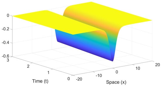
Figure 1.
An example of the traveling waves solution of the Korteweg–de Vries equation, in (2), is plotted as a function of space and time.
Machine learning methods have been applied to PDEs many times [33] and in numerous applications [34,35]. Several recent works have used machine learning methods to find the underlying PDE [18,20,25,26,36,37]. Many recent works have aimed to improve the accuracy of solutions to PDEs [15,19,21,22,23,24,25,38,39]. The machine learning models and approaches vary throughout these works such as the use of a residual network [37,40], a new proposed network called PDE-Net [36], a neural network based on Lie groups [27], a multilayer feed-forward neural network [34], and an unsupervised learning [41] approach [42]. Some approaches combine deep neural networks with other methods such as regression models [20] and Galerkin methods [43]. Several works have implemented the physics-informed neural networks (PINNs) approach [19,21,22,24,25,44,45], as proposed by Raissi et al. [39]. PINNs incorporate the PDE and boundary conditions into the objective or loss function to preserve the physics of the equation [19,22,39,46]. Variations within the PINN framework exist to include the gradient optimized [24] and parareal [47] PINNs. An important note to make about PINNs is that the machine learning models represent the solution as a neural network, which are functions of x and t. In this work, a neural network is used to model the stencil weights as a function of the unknown solution u.
Deep learning models, also known as deep neural networks, are very common machine learning models used in problems involving PDEs [15,25,33,48]. Historically, deep neural networks were defined to have more than two hidden layers [49,50]. With today’s technology, the number of layers can be well into the double digits, so a neural network with three or four hidden layers may be considered “simple”. Um et al. [33] use a model with 22 layers. On the lower end, Bar-Sinai et al. [15] use a three-layer neural network. Raissi et al. [25] use two deep neural networks, one with five layers and the other with only two. Raissi et al. [48] provide results using different numbers of layers in their model. The drawbacks to using deep neural networks may include having insufficient training data, slow training time, and/or overfitting [49,50]. This paper uses a single-layer neural network, which is considered a simple neural network, and which has 16 unknown coefficients.
The numerical method of this paper uses a fixed stencil width for the spatial discretization (as opposed to variable as in [15]) and bases the time-stepping algorithm on a second-order implicit-explicit scheme (IMEX2) so as to have an unbounded stability region [11]. Many recent numerical machine learning works use fourth-order Runge–Kutta (RK4) [21,23,25,39,46], presumably for its temporal accuracy, but we find the stability properties to be of greater importance for this training procedure, hence IMEX2 [11,51,52]. Other second-order time-stepping algorithms exist, such as RK2, and could be used in future studies but may lack the stability properties offered by IMEX2 [11]. In addition to choosing a time-stepper with an unbounded stability region, the machine learning network is built in such a way as to preserve the operator’s anti-symmetry, guaranteeing eigenvalues which live in the stability region of the scheme. The resulting scheme is stable for all time, with no limitations on the time step size k (time step is limited in [15]).
The machine-learned numerical method is compared in performance against classical methods, here finite difference and Fourier collocation. Several other works have established methodologies that effectively use machine learning to solve various problems associated with PDEs but do not compare performance with classical methods [19,21,22,23,24,39,44]. The method in this paper is observed to outperform these two classic methods, but comes with a restriction that the initial data must be close to the training set. This is an expected trade-off based on how the scheme was designed.
Training and test data sets can be generated in various ways. In several works, an initial set of data is generated using a classical method such as from finite difference or spectral methods [20,21,22,23,25,36], and the training and test data sets are both taken from that initial set [22,23,25,43]. Another approach includes generating one set of solutions to train on and another entirely different set to test on [43]. One last approach is training and testing on data randomly sub-sampled from several different initial sets of solutions [15]. This paper first uses a short time interval of a single solution trajectory for training, then tests on both the long time dynamics of the trained trajectory and those of other initial data. Also tested were training routines that used short time intervals from two solution trajectories.
The remainder of the paper is organized as follows: Section 2 discusses the architecture of the scheme, the machine learning model, and the procedure for creating the solutions to be used for training and testing. Section 3 discusses the outcomes of using different sets of initial data when training and testing the model and the performance compared to finite difference and spectral methods. Finally, Section 4 provides conclusions about the use of this method for approximating solutions to PDEs on coarse grids and future research.
2. Numerical Method
2.1. Initial Data
Both training and testing data was generated via highly-resolved numerical simulations. The numerical method used for this data was Fourier collocation for spatial derivatives and an IMEX2 time-stepping scheme, which has the form
where n denotes a point in space and the superscripts denote the solutions evaluated at the point n, and k is the temporal step size [52]. This scheme uses an implicit scheme (trapezoidal) for the linear term of the KdV equation, denoted as in (3), and an explicit scheme (leap frog) for the nonlinear term, denoted as in (3). This method is not self-starting, so for the first time step, a first-order IMEX scheme was used with the form
which uses the backward Euler method for the linear term and the forward Euler method for the nonlinear term [52]. For a small nonlinearity, the IMEX2 scheme becomes the trapezoidal scheme, which is stable on the entire left-half of the -plane, to include the imaginary axis. Since the eigenvalues of the KdV equation are all pure imaginary, the IMEX2 scheme is linearly stable (with an unbounded stability region [11]).
All simulations in this work were conducted on a Windows 10 laptop computer and Mac Pro with macOS Monterey using MATLAB version R2022b. The initial data are all localized and exponentially decaying. The total number of spatial points was sampled logarithmically in powers of two. The infinite spatial domain was approximated by , and 60. For each domain size, the initial highly-resolved solution sets consist of 512 spatial steps and 30,001 temporal steps. Spatial and temporal data were sub-sampled from highly-resolved numerical simulations to build the training and test data sets for the machine learning model. The temporal data is sampled every 10th time step and spatial data is sampled to achieve grids with 16, 32, and 64 points for each domain size. The resulting highly-resolved, but coarsely gridded, data were used for both training and testing.
2.2. Model Set-Up
Many recent works build numerical methods with a machine learning component [18,19,20,21,22,23,24,25,26,36,39,43,46]. In contrast to these previous works, the machine learning model herein is applied solely to the linear spatial derivative term. In this section, we describe the construction of this model. The model is built off of a finite difference method for the third derivative term of the equation, specifically a second-order centered difference approximation [53], which has the following form:
This approximation uses a five-point stencil with coefficients , 1, 0, , and . Let and Then, Equation (5) can be written as
and the differentiation matrix is the matrix such that
for j from 1 to N. is a circulant matrix, so the coefficients are the same in every row since they have no dependence on j [3]. Additionally, is anti-symmetric; that is, a matrix such that where the superscript T denotes the transpose.
In this paper, the coefficients and are replaced with optimal weights found using machine learning that reduce error on coarse grids. The model function used to find the weights has the form
which is a vector-valued function of length two, where is a vector of length two of unknown coefficients, and are matrices of unknown coefficients with dimensions and , respectively, and is an activation function which acts on the input vector component-wise. is a matrix with entries
with accounting for the periodicity, and where is the Kronecker delta defined as
so that applied to evaluates the five adjacent function values,
thus the model design preserves the support of the finite difference stencil (Equation (7) will look different when or N due to periodicity at the boundaries, and this change is handled explicitly in the definition of ).
The differentiation matrix of the machine learning model, denoted , is enforced to be anti-symmetric so that its eigenvalues lie on the imaginary axis. This gives a stable scheme, but also enforces an added consistency with the PDE. For each j from 1 to N, the output of the vector function of the machine learning model is
Unlike in the finite difference method, the coefficients found using the machine learning model are different for every row, since they depend on . Therefore, has the following form:
This results in a machine learning approximation for the third derivative term as follows:
This approximation is substituted into the IMEX2 scheme, replacing the finite difference approximation for the third derivative term, which gives
This scheme differs from the IMEX2 scheme in Equation (3) since g now depends on u at two different time steps. Since this scheme is not self-starting, the following time-stepping scheme is used for the first time step:
2.3. Objective Function and Error
The objective function used for training is the truncation error of Equation (9), evaluated by using the highly-resolved numerical simulations as a proxy for the exact solution. The nonlinear function f is approximated using a second-order finite difference approximation for first derivatives. Minimization techniques are then applied to the scheme to optimize the model’s truncation error.
Gradient-based optimization algorithms for the objective function are commonly used to include stochastic gradient descent [19,24,43], Adam optimizer [19,20,23,42], Broyden–Fletcher–Goldfarb–Shanno (BFGS) [27], and Limited-memory BFGS [19,21,22,26,28,39,44]. For this paper, the gradient-based method used to minimize the truncation error is the steepest descent algorithm. The tolerance for the algorithm is one-tenth of the truncation error of the corresponding finite difference method (where and and are matrices whose entries are all zeros). This finite difference method was also used as an initial guess in the optimization routines.
In addition to the truncation error, the forward error is also used as a measure of performance. The forward error is calculated by taking the 2-norm of the difference between the approximated solutions found using each method and the highly-resolved Fourier solution, :
To summarize, the training data from the highly-resolved Fourier simulations is used as a proxy for the exact solution, then the truncation error of (9) is minimized. The weights (i.e., the entries of , and ) are optimized via steepest descent. Once these weights are found, they are used in Equation (9) to evolve new initial data. The results are compared to finite difference and Fourier collocation using the same time-stepper and spatial discretization.
3. Results
Two training routines were evaluated. One training method used a single solution trajectory over a short time interval. The second used two solution trajectories (again over a short time interval). In both scenarios, the trained numerical method was evaluated against the parent finite difference method and Fourier collocation both at and near the training initial data, for short and long times.
In both training routines, the set of initial data trained and tested on is of the form
where A is a changeable parameter. When , this is a soliton solution of the KdV equation traveling at speed c. For , the solution is not a traveling wave, and has a more complicated trajectory. The model was trained and tested using both traveling wave and non-traveling wave initial data.
The activation function used in simulations in this paper was the hyperbolic tangent function, which resulted in the machine learning model function
This is a common activation function [50] and is used in several other recent works involving PDEs [15,19,20,21,22,25,43,44,45].
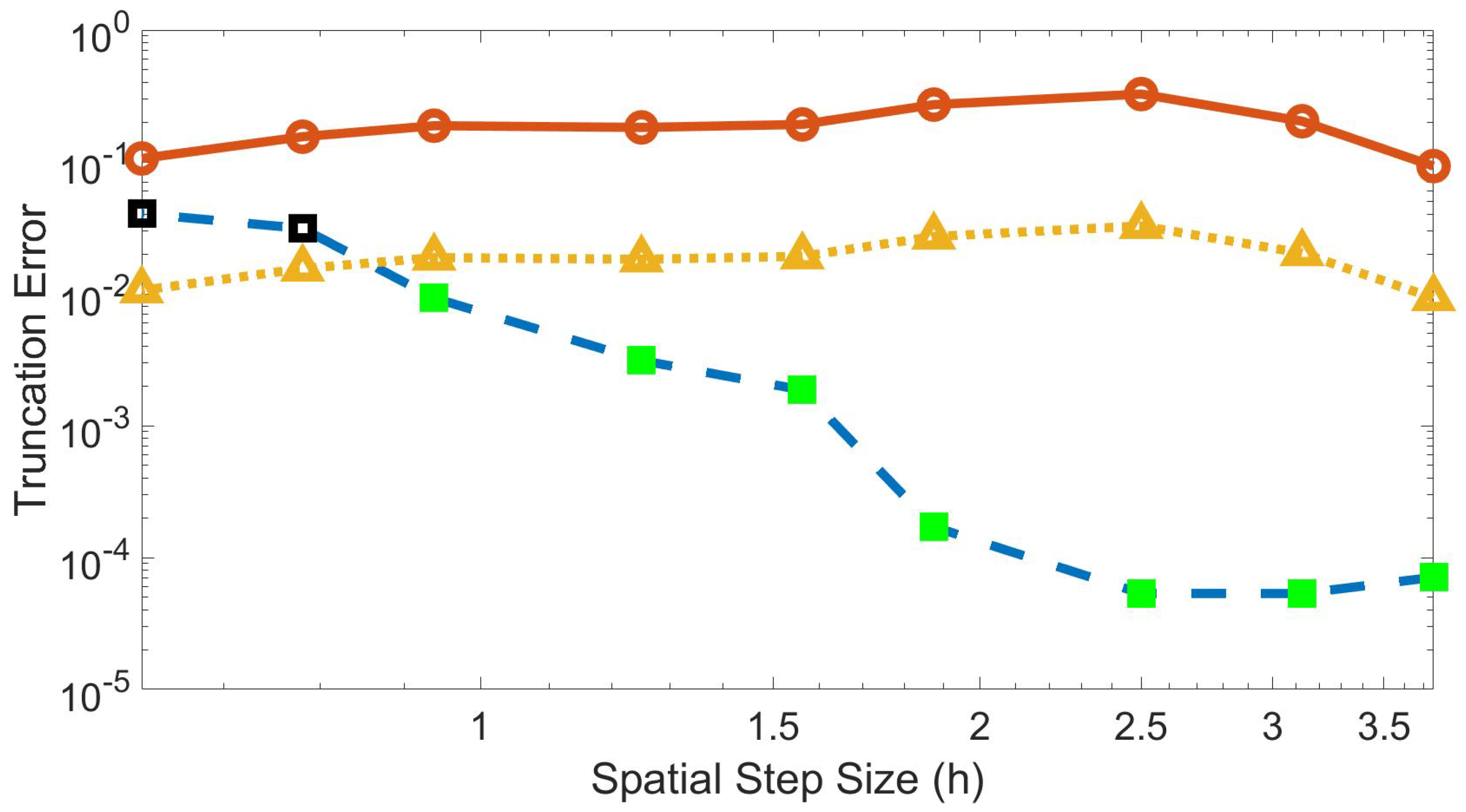
Figure 2 shows an example plot of the truncation error through the training time using the trained speed and trained . For larger h values, the method converged to below the threshold of one-tenth the truncation error value for the finite difference method. For smaller h, the method is unable to converge below this threshold. For these values, the model may need to be amended by adding more layers or by using a broader stencil. For the remaining figures shown in this paper, a step size of is used, which uses a grid of 16 data points.
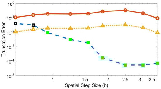
Figure 2.
Truncation error for the machine learning and finite difference methods at each spatial step size through training time using trained speed and trained . Blue dashed line with square markers is the machine learned error with green solid denoting convergence of minimization algorithm and black outline denoting non-convergence; solid red line with circle markers is the finite difference error; yellow dotted line with triangle markers is one-tenth the finite difference error.
In Figure 2, the trained scheme significantly outperforms the finite difference method on coarse grids, but the gains decrease with step size. There is no gain in using this methodology as (nor is any convergence study conducted in the small h limit). The remainder of the paper considers a fixed model with fixed step size, where the machine-learned procedure outperforms Fourier collocation and classic finite difference. To decrease errors beyond those presented, one could consider a convergence study in the number of layers or the breadth of the layers in the machine learning model. Generally, more layers in neural networks can provide more accurate approximations [49]; however, the training cost increases with layer width and depth. The effect of more or broader layers is a future research avenue.
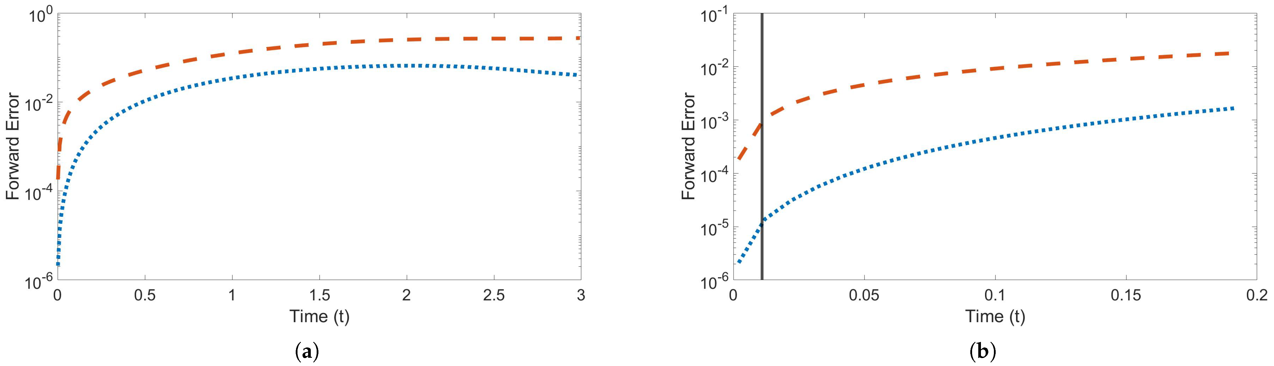
Figure 3 shows the forward error over time using the trained speed and , with Figure 3a showing the error through time . The forward error of the machine learned model is less than that of the finite difference method for the entire time interval, even though the method was only trained on a very small portion of the entire time interval, as shown in Figure 3b.
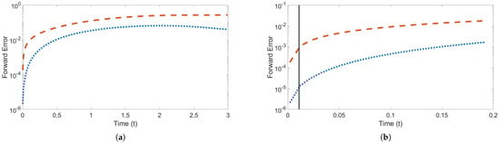
Figure 3.
Forward error over time training and testing on speed and . Red dashed line is the finite difference error; blue dotted line is the machine learned error. Dark gray vertical line indicates the end of the training time interval (a) Error through time . (b) Error through time .
3.1. Single Solution Trajectory
When the model was trained on a single solution trajectory, one pair from (10), the training set was the the first 12 consecutive time steps ( to ) of a coarse sampling of the highly-resolved solution. The model was tested using other initial data (nearby pairs) and for longer times.
Discussion
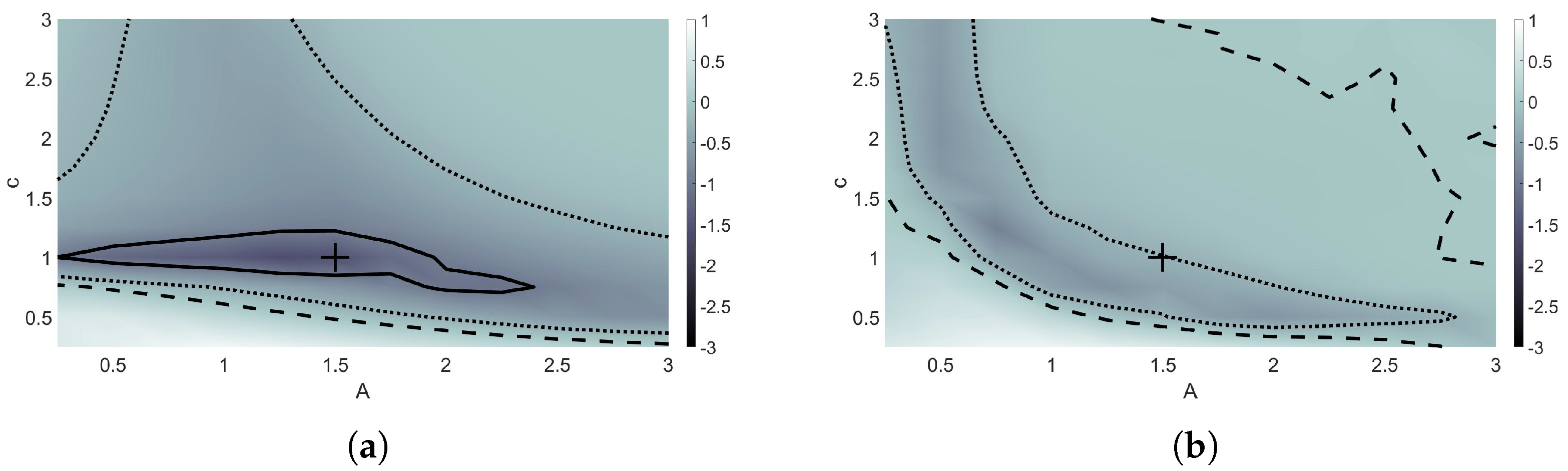
The model was trained on an initial highly-resolved solution set using a non-solitary wave, with and . Figure 4 shows the forward error rates for each c and A that were trained and tested on. The forward error rate was calculated by taking the logarithm of the absolute maximum forward error of the machine learning model over the entire time interval divided by the absolute maximum forward error of the finite difference model over the time interval. In Figure 4, the solutions with c and A values within the region surrounded by the solid black lines performed 10 times better than the finite difference method. From Figure 4a, a range of solutions found by testing on varying c and A values around the solution that was trained on, which is indicated by the ‘+’, also have lower forward errors when using the optimal coefficients found during minimization. The only areas shown where the machine learning model did not outperform finite difference methods were for most A values used in combination with speeds less than 0.75.
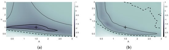
Figure 4.
Forward error rate plots comparing performance of finite different methods and the machine learning model. Model trained using and , indicated by “+”. Model tested using c and A values ranging from 0.25 to 3. Contours indicate initial data where the machine learning model performs 10 times better than (solid), 2 times better than (dotted), and equivalent to (dashed) finite difference methods. (a) Maximum forward error rate through training time interval. (b) Maximum forward error rate through time .
At time , the machine learning model continued to outperform finite difference methods for most pairs plotted in Figure 4b; however, the region of solutions that performed 10 times better than finite difference methods has essentially become non-existent. A region of pairs still performed at least two times better than the finite difference method, as indicated by the dotted contours.
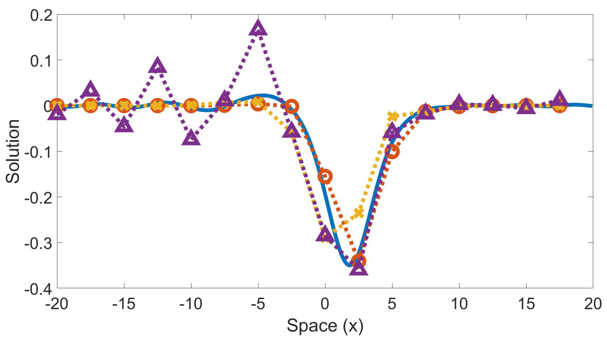
Figure 5 shows the wave solution at time using test values and comparing the highly-resolved Fourier method, finite difference method, the machine learning model, and an under-resolved Fourier model. The machine learning model outperformed both classical methods in predicting the behavior of the wave solution at a time well beyond the interval it was trained on and on a coarse grid. The approximate computation time for each method is as follows: 0.352 s for machine-learned; 0.344 s for finite difference; and 0.037 s for under-resolved Fourier. Several other initial data were used for training and testing, both on solitary and non-solitary waves, with similar results.

Figure 5.
Time evolution of a wave trained on a non-solitary wave ( and ) and tested on a different non-solitary wave ( and ). Solution at time . Solid blue line is the highly-resolved Fourier; dotted red line with “o” markers is the machine learning model; dotted yellow line with “x” markers is finite difference; dotted purple line with “Δ” markers is Fourier on coarse grid. The machine-learned model relative forward error is 0.1322. The finite difference relative forward error is 0.3934. The coarse Fourier relative forward error is 0.5663.
It is important to note that the methodology in this paper has been set up so that the truncation error of the machine learning model will always be less than that of the finite difference method when the minimization method converges. By the Lax Equivalence Theorem, the forward error of a method is bounded by the sum of the accumulated truncation error of that method [2,11,12], e.g.,
In (12), is the maximal growth rate of errors from one step to the next (stable schemes have ), is the exact solution, is the numerical solution at time , and is the truncation error at time . As a consequence of (12), the forward error of the machine learning model must be less than the accumulated truncation error of the model, and the forward error of the finite difference method must be less than the accumulated truncation error of the finite difference method; however, nothing can be said about the ordering of the forward error of the two methods. In other words, the methodology does not guarantee that the forward error of the machine learning model will be less than the forward error of the finite difference method. That said, the spectrum of the linear operators in all cases (machine learned model, finite difference, and Fourier) lie exactly on the boundary of the linear stability region of IMEX2, so the growth rates of truncation errors from step to step are exactly one , and there is no difference in the temporal stability of these schemes. The proof of the Lax Equivalence Theorem uses the triangle inequality, so in principle there could be more cancellation in one scheme than another. We, however, observe that the forward error and the accumulated truncation error are matched closely for all methods. Even though the machine learned model is trained using the truncation error as the objective function, it effectively also minimizes the forward error (Direct minimization of the forward error would be significantly more expensive as it would require running the scheme (with its matrix inversions) during each evaluation of the objective function in the training).
3.2. Two Sets of Initial Data
In addition to training on a single solution trajectory, we tested models that were trained on two sets of initial data simultaneously. The results of this training algorithm presented here used pairs and , so the model is training on two solitary waves of different speeds. The data from the first seven time steps ( to ) of each set of solutions were used to train the model. To create the objective function for two sets of solutions, the truncation error for each is combined to create a multi-objective minimization problem. The error using each solution is calculated individually then normalized by dividing by the square of the largest absolute solution from the respective training data set before being added together to create the objective function. In the steepest descent algorithm, the threshold is one-tenth of the minimum finite difference truncation error between the two solutions. This minimization process allows the algorithm to find the optimal coefficients that minimize both initial sets of data simultaneously.
Discussion
Figure 6 shows the forward error rate plots for training on the two solutions. In Figure 6a, by training on two initial solutions with different speeds, a larger range of speeds used in combination with varying A values were able to outperform the finite difference method by at least 10 times through the training time, as compared to training using only one solution with one speed, as was performed in Figure 4. As the wave propagates to time , there were no areas where the machine learning model outperformed the finite difference method by 10 times or more, although a majority of pairs shown in Figure 6b resulted in a method that outperformed the classical method.
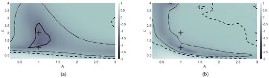
Figure 6.
Forward error rate plots comparing performance of finite different methods and the machine learning model. Model trained using speeds and and , indicated by “+”. Model tested using c and A values ranging from 0.25 to 3. Contours indicate initial data where the machine learning model performs 10 times better than (solid), 2 times better than (dotted), and equivalent to (dashed) finite difference methods. (a) Maximum forward error rate through end of training time interval. (b) Maximum forward error rate through time .
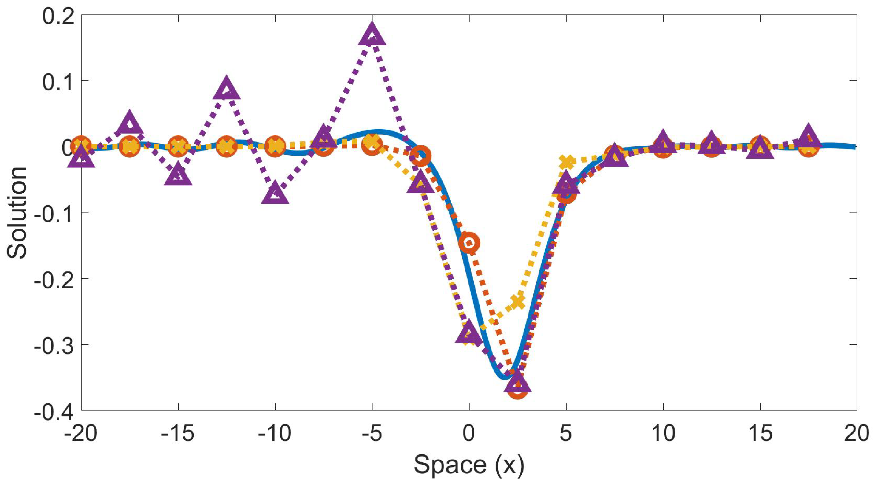
A wave solution is shown in Figure 7 at time , which tests the model using and . The model outperformed both the finite difference and under-resolved Fourier methods in predicting the behavior of the highly-resolved solution.

Figure 7.
Time evolution of a wave trained using and and and tested on a wave using and . Solution at time . Solid blue line is the highly-resolved Fourier collocation method; dotted red line with “o” markers is the machine learning model; dotted yellow line with “x” markers is the finite difference result; dotted purple line with “Δ” markers are a Fourier collocation on the coarse grid. The machine-learned model relative forward error is 0.0452. The finite difference relative forward error is 0.1003. The coarse Fourier relative forward error is 0.1444.
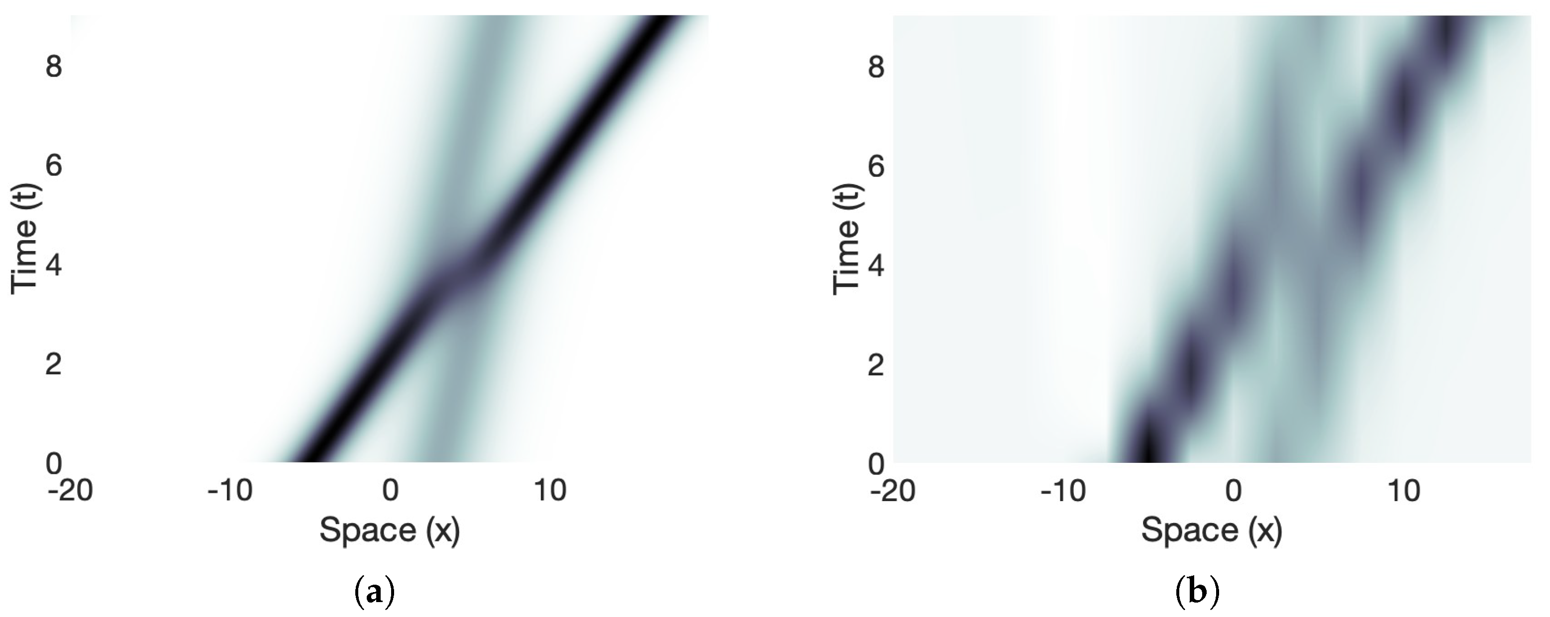
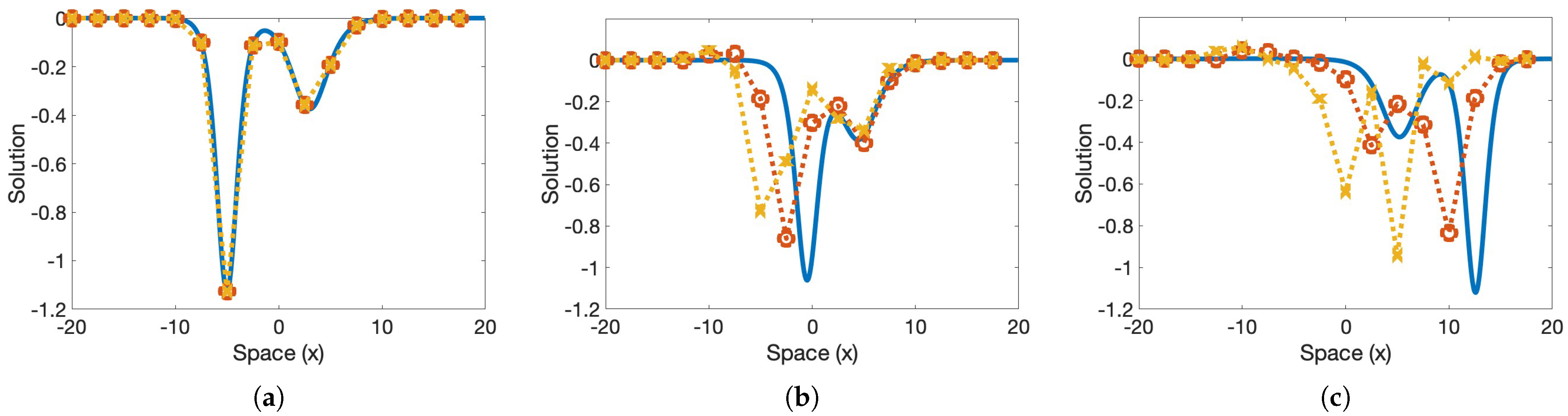
The optimal coefficients found by training on the previous two initial data were tested using two different sets of data, where and . Figure 8b shows the collision of the two solitons as they propagate through space and time using the machine learned model on a coarse grid. Despite the model not being trained on a collision, it is still able to pick up on the overall dynamics, displaying the new trajectories of each wave after the collision occurs. Figure 9 shows the time evolution of the waves, comparing the machine-learned solution to the highly-resolved Fourier at different times throughout the interval. The model is a bit slow at picking up the trajectories of the waves, but is able to recognize the collision between the solitons.
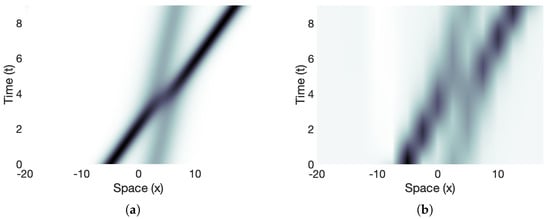
Figure 8.
Simulation of a collision between solitons with speeds and . (a) Highly-resolved Fourier dynamics. (b) Machine learned dynamics. Coefficients found by training on initial data and ; tested using and .

Figure 9.
The collision of two solitary waves is depicted. The machine learned model was trained using two single solitary wave trajectories at and ; the colliding waves in this test had different amplitudes from the trained trajectories, and , and the training did not include a collision. The solid blue line is the highly-resolved Fourier; the dotted red line with “o” markers is the machine learning model; the dotted yellow line with “x” markers is the finite difference result. The solution at time is in panel (a), at in panel (b), and at in panel (c).
4. Conclusions
In this paper, machine learning was utilized to optimize the coefficients of a numerical differencing scheme for the KdV equation. This scheme was trained on a coarse grid and outperformed two classical methods (finite difference and Fourier). Training procedures using a single solution trajectory and a pair of trajectories were implemented. The model was tested on a variety of nearby initial data, both solitary and non-solitary trajectories. A solitary wave collision was also tested. The methodology is expected to be applicable to other nonlinear wave equations. Future work could include using the forward error as the objective function instead of the truncation error; however, this will be more expensive as a matrix inversion will be required for the time-stepping scheme for each iteration in the steepest descent algorithm. Other future work could include training the model on non-consecutive time steps by randomly sampling the initial data to obtain the training and test data sets as has been carried out in several recent works [19,21,22,23,25,36,37,39]. This could also include randomly sampling from several initial data sets. Additionally, more layers could be added to the model. A different activation function could be used, e.g., leaky or standard rectified linear unit [15,44,45,46]. The method also naturally generalizes to broader stencils.
Author Contributions
Conceptualization, B.F.A.; methodology, K.O.F.W. and B.F.A.; software, K.O.F.W.; validation, K.O.F.W. and B.F.A.; formal analysis, K.O.F.W. and B.F.A.; writing—original draft preparation, K.O.F.W. and B.F.A.; writing—review and editing, K.O.F.W. and B.F.A.; visualization, K.O.F.W.; supervision, B.F.A.; project administration, B.F.A.; funding acquisition, B.F.A. All authors have read and agreed to the published version of the manuscript.
Funding
B.F.A. acknowledges funding from the APTAWG, under the program “Simulation of laser propagation in reactive media”.
Data Availability Statement
MATLAB code is available upon request.
Acknowledgments
The authors would like to thank Jonah Reeger for helpful conversations.
Conflicts of Interest
This report was prepared as an account of work sponsored by an agency of the United States Government. Neither the United States Government nor any agency thereof, nor any of their employees, make any warranty, express or implied, or assume any legal liability or responsibility for the accuracy, completeness, or usefulness of any information, apparatus, product, or process disclosed, or represent that its use would not infringe privately owned rights. Reference herein to any specific commercial product, process, or service by trade name, trademark, manufacturer, or otherwise does not necessarily constitute or imply its endorsement, recommendation, or favoring by the United States Government or any agency thereof. The views and opinions of authors expressed herein do not necessarily state or reflect those of the United States Government or any agency thereof.
References
- Thomée, V. From finite differences to finite elements: A short history of numerical analysis of partial differential equations. In Numerical Analysis: Historical Developments in the 20th Century; Elsevier: Amsterdam, The Netherlands, 2001; pp. 361–414. [Google Scholar]
- Fornberg, B. A Practical Guide to Pseudospectral Methods; Number 1; Cambridge University Press: Cambridge, UK, 1998. [Google Scholar]
- Trefethen, L.N. Spectral Methods in MATLAB; SIAM: Philadelphia, PA, USA, 2000. [Google Scholar]
- LeVeque, R.J. Finite Difference Methods for Ordinary and Partial Differential Equations: Steady-State and Time-Dependent Problems; SIAM: Philadelphia, PA, USA, 2007. [Google Scholar]
- Milewski, P.A.; Tabak, E.G. A pseudospectral procedure for the solution of nonlinear wave equations with examples from free-surface flows. SIAM J. Sci. Comput. 1999, 21, 1102–1114. [Google Scholar]
- Jin, S.; Xin, Z. The relaxation schemes for systems of conservation laws in arbitrary space dimensions. Commun. Pure Appl. Math. 1995, 48, 235–276. [Google Scholar]
- Dutykh, D.; Pelinovsky, E. Numerical simulation of a solitonic gas in KdV and KdV–BBM equations. Phys. Lett. A 2014, 378, 3102–3110. [Google Scholar]
- Akers, B.; Liu, T.; Reeger, J. A radial basis function finite difference scheme for the Benjamin–Ono equation. Mathematics 2020, 9, 65. [Google Scholar]
- Akers, B.F.; Ambrose, D.M. Efficient computation of coordinate-free models of flame fronts. ANZIAM J. 2021, 63, 58–69. [Google Scholar]
- Akers, B. The generation of capillary-gravity solitary waves by a surface pressure forcing. Math. Comput. Simul. 2012, 82, 958–967. [Google Scholar]
- Novak, K. Numerical Methods for Scientific Computing; Lulu Press: Morrisville, NC, USA, 2017. [Google Scholar]
- Smith, G.D. Numerical Solution of Partial Differential Equations: Finite Difference Methods; Oxford University Press: Oxford, UK, 1985. [Google Scholar]
- Quarteroni, A.; Sacco, R.; Saleri, F. Numerical Mathematics; Springer Science & Business Media: Berlin/Heidelberg, Germany, 2010; Volume 37. [Google Scholar]
- Pathak, J.; Mustafa, M.; Kashinath, K.; Motheau, E.; Kurth, T.; Day, M. Using machine learning to augment coarse-grid computational fluid dynamics simulations. arXiv 2020, arXiv:2010.00072. [Google Scholar]
- Bar-Sinai, Y.; Hoyer, S.; Hickey, J.; Brenner, M.P. Learning data-driven discretizations for partial differential equations. Proc. Natl. Acad. Sci. USA 2019, 116, 15344–15349. [Google Scholar]
- Nordström, J.; Ålund, O. Neural network enhanced computations on coarse grids. J. Comput. Phys. 2021, 425, 109821. [Google Scholar]
- Korteweg, D.J.; De Vries, G. XLI. On the change of form of long waves advancing in a rectangular canal, and on a new type of long stationary waves. Lond. Edinb. Dublin Philos. Mag. J. Sci. 1895, 39, 422–443. [Google Scholar]
- Rudy, S.H.; Brunton, S.L.; Proctor, J.L.; Kutz, J.N. Data-driven discovery of partial differential equations. Sci. Adv. 2017, 3, e1602614. [Google Scholar]
- Guo, Y.; Cao, X.; Liu, B.; Gao, M. Solving partial differential equations using deep learning and physical constraints. Appl. Sci. 2020, 10, 5917. [Google Scholar]
- Xu, H.; Chang, H.; Zhang, D. DL-PDE: Deep-learning based data-driven discovery of partial differential equations from discrete and noisy data. arXiv 2019, arXiv:1908.04463. [Google Scholar]
- Bai, Y.; Chaolu, T.; Bilige, S. Physics informed by deep learning: Numerical solutions of modified Korteweg-de Vries equation. Adv. Math. Phys. 2021, 2021, 1–11. [Google Scholar]
- Zhang, Y.; Dong, H.; Sun, J.; Wang, Z.; Fang, Y.; Kong, Y. The new simulation of quasiperiodic wave, periodic wave, and soliton solutions of the KdV-mKdV Equation via a deep learning method. Comput. Intell. Neurosci. 2021, 2021, 8548482. [Google Scholar]
- Li, J.; Chen, Y. A deep learning method for solving third-order nonlinear evolution equations. Commun. Theor. Phys. 2020, 72, 115003. [Google Scholar]
- Li, J.; Chen, J.; Li, B. Gradient-optimized physics-informed neural networks (GOPINNs): A deep learning method for solving the complex modified KdV equation. Nonlinear Dyn. 2022, 107, 781–792. [Google Scholar]
- Raissi, M. Deep hidden physics models: Deep learning of nonlinear partial differential equations. J. Mach. Learn. Res. 2018, 19, 932–955. [Google Scholar]
- Raissi, M.; Karniadakis, G.E. Hidden physics models: Machine learning of nonlinear partial differential equations. J. Comput. Phys. 2018, 357, 125–141. [Google Scholar]
- Wen, Y.; Chaolu, T. Learning the nonlinear solitary wave solution of the Korteweg-de Vries equation with novel neural network algorithm. Entropy 2023, 25, 704. [Google Scholar]
- Gurieva, J.; Vasiliev, E.; Smirnov, L. Improvements of accuracy and convergence speed of AI-based solution for the Korteweg-De Vries equation. ББК 22.18 я43 М34 2022, 5, 49336041. [Google Scholar]
- Wu, H.; Xu, H. Studies of wave interaction of high-order Korteweg-de Vries equation by means of the homotopy strategy and neural network prediction. Phys. Lett. A 2021, 415, 127653. [Google Scholar]
- Remoissenet, M. Waves Called Solitons: Concepts and Experiments; Springer Science & Business Media: Berlin/Heidelberg, Germany, 2013. [Google Scholar]
- Markowski, P.; Richardson, Y. Mesoscale Meteorology in Midlatitudes; John Wiley & Sons: Hoboken, NJ, USA, 2011; Volume 2. [Google Scholar]
- Holton, J. An Introduction to Dynamic Meteorology; International Geophysics; Elsevier Science: Amsterdam, The Netherlands, 2004. [Google Scholar]
- Um, K.; Brand, R.; Fei, Y.R.; Holl, P.; Thuerey, N. Solver-in-the-loop: Learning from differentiable physics to interact with iterative pde-solvers. Adv. Neural Inf. Process. Syst. 2020, 33, 6111–6122. [Google Scholar]
- Khodadadian, A.; Parvizi, M.; Teshnehlab, M.; Heitzinger, C. Rational Design of Field-Effect Sensors Using Partial Differential Equations, Bayesian Inversion, and Artificial Neural Networks. Sensors 2022, 22, 4785. [Google Scholar]
- Noii, N.; Khodadadian, A.; Ulloa, J.; Aldakheel, F.; Wick, T.; Francois, S.; Wriggers, P. Bayesian inversion with open-source codes for various one-dimensional model problems in computational mechanics. Arch. Comput. Methods Eng. 2022, 29, 4285–4318. [Google Scholar]
- Long, Z.; Lu, Y.; Ma, X.; Dong, B. Pde-net: Learning pdes from data. In Proceedings of the International Conference on Machine Learning, PMLR, Stockholm, Sweden, 10–15 July 2018; pp. 3208–3216. [Google Scholar]
- Wu, K.; Xiu, D. Data-driven deep learning of partial differential equations in modal space. J. Comput. Phys. 2020, 408, 109307. [Google Scholar]
- Yang, X.; Wang, Z. Solving Benjamin–Ono equation via gradient balanced PINNs approach. Eur. Phys. J. Plus 2022, 137, 864. [Google Scholar]
- Raissi, M.; Perdikaris, P.; Karniadakis, G.E. Physics-informed neural networks: A deep learning framework for solving forward and inverse problems involving nonlinear partial differential equations. J. Comput. Physics 2019, 378, 686–707. [Google Scholar]
- He, K.; Zhang, X.; Ren, S.; Sun, J. Deep residual learning for image recognition. In Proceedings of the IEEE Conference on Computer Vision and Pattern Recognition, Las Vegas, NV, USA, 26 June–1 July 2016; pp. 770–778. [Google Scholar]
- James, G.; Witten, D.; Hastie, T.; Tibshirani, R. An Introduction to Statistical Learning; Springer: Berlin/Heidelberg, Germany, 2013; Volume 112. [Google Scholar]
- Bar, L.; Sochen, N. Unsupervised deep learning algorithm for PDE-based forward and inverse problems. arXiv 2019, arXiv:1904.05417. [Google Scholar]
- Sirignano, J.; Spiliopoulos, K. DGM: A deep learning algorithm for solving partial differential equations. J. Comput. Phys. 2018, 375, 1339–1364. [Google Scholar]
- Kadeethum, T.; Jørgensen, T.M.; Nick, H.M. Physics-informed neural networks for solving nonlinear diffusivity and Biot’s equations. PLoS ONE 2020, 15, e0232683. [Google Scholar]
- Beck, C.; Hutzenthaler, M.; Jentzen, A.; Kuckuck, B. An overview on deep learning-based approximation methods for partial differential equations. arXiv 2020, arXiv:2012.12348. [Google Scholar]
- Blechschmidt, J.; Ernst, O.G. Three ways to solve partial differential equations with neural networks—A review. GAMM-Mitt. 2021, 44, e202100006. [Google Scholar]
- Meng, X.; Li, Z.; Zhang, D.; Karniadakis, G.E. PPINN: Parareal physics-informed neural network for time-dependent PDEs. Comput. Methods Appl. Mech. Eng. 2020, 370, 113250. [Google Scholar]
- Raissi, M.; Perdikaris, P.; Karniadakis, G.E. Physics informed deep learning (part i): Data-driven solutions of nonlinear partial differential equations. arXiv 2017, arXiv:1711.10561. [Google Scholar]
- Goodfellow, I.; Bengio, Y.; Courville, A. Deep Learning; Adaptive Computation and Machine Learning Series; MIT Press: Cambridge, MA, USA, 2017; pp. 321–359. [Google Scholar]
- Géron, A. Hands-on Machine Learning with Scikit-Learn, Keras, and TensorFlow: Concepts, Tools, and Techniques to Build Intelligent Systems; O’Reilly Media, Inc.: Newton, MA, USA, 2019. [Google Scholar]
- Ascher, U.M.; Ruuth, S.J.; Spiteri, R.J. Implicit-explicit Runge-Kutta methods for time-dependent partial differential equations. Appl. Numer. Math. 1997, 25, 151–167. [Google Scholar] [CrossRef]
- Ascher, U.M.; Ruuth, S.J.; Wetton, B.T.R. Implicit-explicit methods for time-dependent partial differential equations. SIAM J. Numer. Anal. 1995, 32, 797–823. [Google Scholar]
- Fornberg, B. Generation of finite difference formulas on arbitrarily spaced grids. Math. Comput. 1988, 51, 699–706. [Google Scholar]


Disclaimer/Publisher’s Note: The statements, opinions and data contained in all publications are solely those of the individual author(s) and contributor(s) and not of MDPI and/or the editor(s). MDPI and/or the editor(s) disclaim responsibility for any injury to people or property resulting from any ideas, methods, instructions or products referred to in the content. |
© 2023 by the authors. Licensee MDPI, Basel, Switzerland. This article is an open access article distributed under the terms and conditions of the Creative Commons Attribution (CC BY) license (https://creativecommons.org/licenses/by/4.0/).