Synchronization of Markov Switching Inertial Neural Networks with Mixed Delays under Aperiodically On-Off Adaptive Control

Abstract

In this paper, the issue of exponential synchronization in Markov switching inertial neural networks with mixed delays is investigated via aperiodically on–off adaptive control. The inertial term is considered, which extends the existing network modes with first-order differential term. Combined with the Lyapunov method, graph theory, and the differential inequalities technique, two types of synchronization criteria are presented which take into account all of the time delay information and reduce the conservativeness. Finally, some numerical simulations are provided in order to show the validity of the theoretical results.

1. Introduction

It is well known that neural networks have been a research hotspot in many fields, such as mathematics, information science, control science, and computer science, as they possess good intelligence characteristics including self-learning ability, a high fault-tolerance rate, associative memory, etc. [1,2,3]. It should be pointed out that most of the neural network models considered in the existing literature are based on the form of first-order differential equations. Second-order differential equations, on the other hand, have a wider range of applications and can greatly enhance the disordered search performance of neural network memory. In the 1990s, Babcock and Westervelt first introduced the inertial term, namely the second-order differential term in a mathematical sense, into neural networks and obtained inertial neural networks (INNs) [4]. INNs have a strong biological and engineering background. For example, the axonal function of squid can be realized by using inductance [5]. Additionally, inductance is introduced into the circuit of a neuron, which can realize functions similar to a space–time filter, band-pass filter and point tuning [6,7,8]. In fact, the existence of an inertia term will lead to more complex dynamic phenomena in the system, such as chaos or bifurcation. Therefore, the study of INNs is a subject worthy of exploration.

Data leakage, including unauthorized information interception and database data theft, frequently happens as a result of the rapid development of data communication. Data transmission secrecy is a very critical topic since issues with data confidentiality have enormous ramifications if they affect financial information, military intelligence, etc. Research shows that synchronization can be successfully applied to communication security, which helps to improve the security of data communication [9]. In engineering applications, synchronization can also be applied to image processing, information science, biotechnology, and other fields [10,11]. In addition, synchronization is also important for the normal operation of neural networks, especially in the fields of image recognition and multi-agent and automatic driving. Therefore, more and more scholars have devoted themselves to the synchronization research of INNs (see [12,13,14]). In general, it is difficult to realize the synchronization of neural networks only through their own topology and coupling strength without external force. Scholars have proposed a variety of control strategies to address this issue, such as adaptive control [15], event-triggered control [16], pulse control [17], and intermittent control [18,19]. On–off control, which is a discontinuous control technique, has the clear benefit of cost savings and is simple to implement in reality. For instance, when the system signal strength is insufficient to meet the terminal’s requirements due to diffusion in the field of communication, the desired outcome can be obtained by adding external control signals. Similarly, the external control can be withdrawn after the signal strength reaches the terminal’s necessary level. It is clear that on–off control can successfully lower control costs, and it has become the focus of research in various fields, such as coupled systems [20], complex networks [21], stochastic neural networks [22], etc. On–off control usually includes periodically on–off control and aperiodically on–off control. In some cases, it is unreasonable to require periodic operation control, while non-periodic control can be more consistent with the application of the actual system.

Markov switching systems are based on the assumption that INNs have a finite number of modes, will switch between modes at different times, and that switching between different modes occurs in the form of a Markov chain. This switching system has strong modeling capability for real life systems that may experience sudden changes in structure and parameters [23,24], such as battlefield management and command, ship steering, communication systems, population dynamics, and national economic models. Therefore, Markov switching inertial neural networks have become a hot topic in the fields of science and engineering. In addition, in the electronic implementation of INNs, the discrete time delay caused by information exchange between neurons is inevitable [25]. In some cases, because molecules of different sizes and lengths form a large number of parallel paths, the neural network has spatial characteristics, which are generally characterized by distributed delay [26]. Therefore, in order to increase the potential application value of the research work, it is necessary to introduce both discrete time delay and distributed time delay (collectively referred to as mixed time delay) when modeling. However, the existence of time delay will also destroy the performance of the neural network, leading to oscillation or instability. Therefore, research on the synchronization and control of Markov switching INNs with mixed delay has irreplaceable theoretical significance and practical value.

In Ref. [27], the author studied the synchronization of a Markov switching inertial neural network through feedback control and discussed its application in secure image communication, but the effect of distributed time delay on synchronization was ignored. Based on periodically intermittent control, Refs. [28,29], respectively, studied the exponential synchronization of time-delayed INNs and reaction–diffusion INNs. However, their models not only did not consider the effect of Markov switching, but also required that the control be periodic, which has certain limitations in practice. To date, research on synchronization and control of Markov switching INNs with mixed delays is still lacking. The adaptive strategy can help the control strength to adjust continuously with the synchronization process so that the INNs can achieve the desired synchronization goal. Therefore, it is necessary and meaningful to consider the synchronization issue in Markov switching INNs with mixed delay by using an aperiodically on–off adaptive control strategy.

The graph theory method is a powerful tool for assessing and designing the global Lyapunov function [30]. In this article, we intend to achieve the synchronization of Markov switching INNs with mixed delay via aperiodically on–off adaptive control. By means of graph theory and the Lyapunov method, some synchronization conditions are presented. The main contributions are as follows:

• The synchronization of Markov switching INNs with mixed delays under aperiodically on–off adaptive control is studied for the first time.
• By using graph theory and the Lyapunov method combined with the differential inequalities technique, some synchronization criteria are derived which are less conservative than those in the existing literature.

The rest of this paper is organized as follows. Section 2 presents some preliminaries. Section 3 derives some novel sufficient criteria through the combination of graph theory and aperiodically on–off adaptive control strategy. Section 4 provides some numerical simulations to show the validity of the theoretical results. Section 5 concludes this paper.

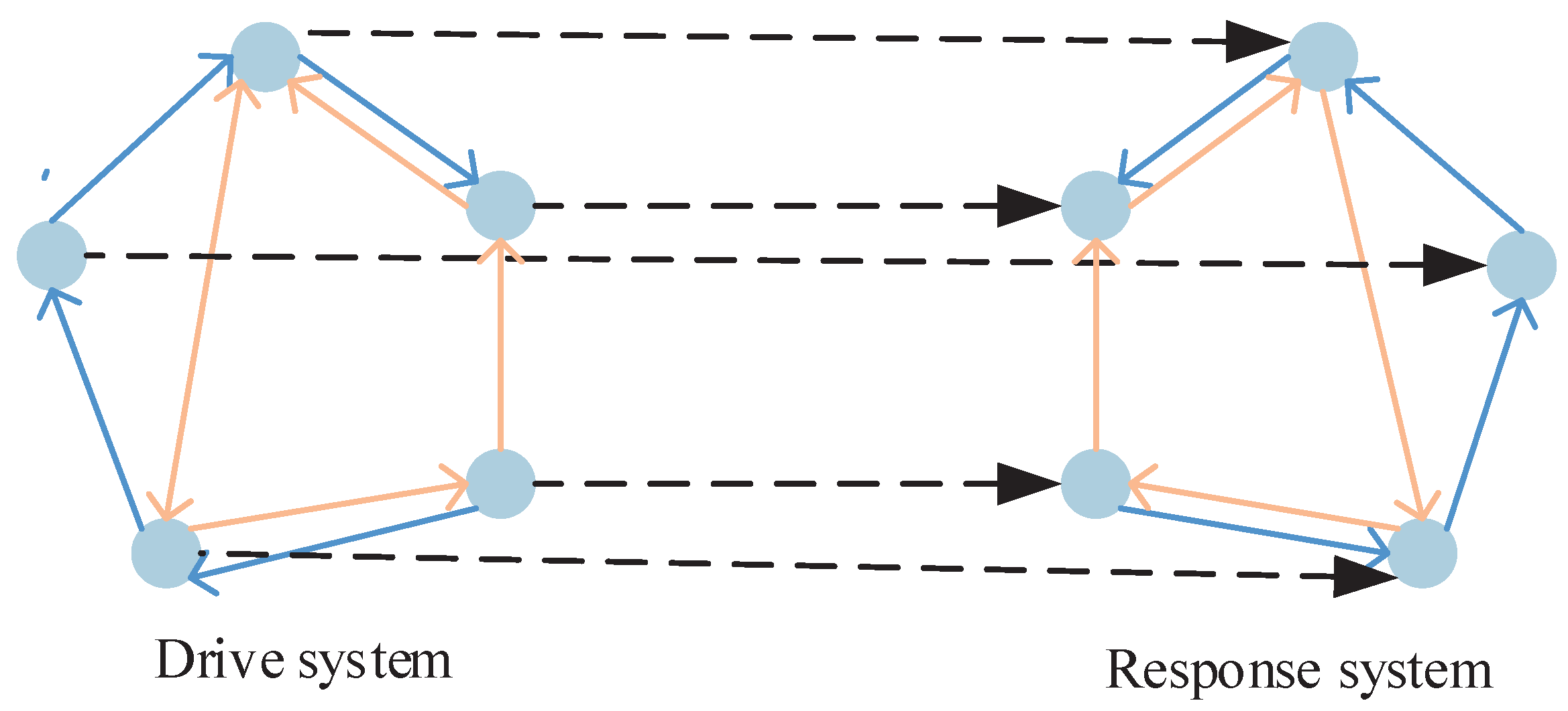
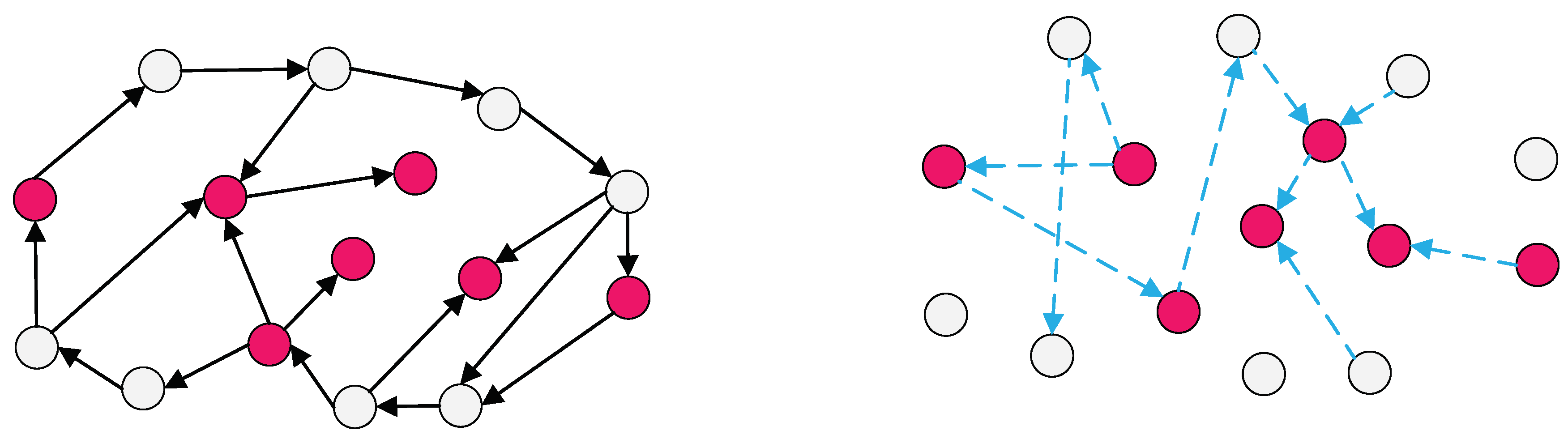
2. Preliminaries and System Models

Throughout this paper, let ${\mathbb{R}}^n$ be the n-dimensional Euclidean space, $|·|$ be the norm, ${\mathbb{R}}^{+}=[0,+\infty )$, $\mathcal{M}=\{1,2,\dots ,m\}$, $\mathbf{L}=\{1,2,\dots ,L\}$, and $a\bigvee b=max\{a,b\}$. Notation $C^{1,2}({\mathbb{R}}^{+}\times {\mathbb{R}}^n\times \mathbf{L},{\mathbb{R}}^n)$ stands for the family of all nonnegative functions $V(t,x,\chi )$ on ${\mathbb{R}}^{+}\times {\mathbb{R}}^n\times \mathbf{L}$, which are continuously twice differentiable in x and once in t. “$\mathrm{T}$” is the transpose of vectors or matrices. Furthermore, $r_t$ is a right continuous Markov chain taking values in a finite state space $\mathbf{L}$ with the transition rate matrix $\mathsf{\Gamma }={(p_{\chi k})}_{L\times L}$ satisfying $p_{\chi k}\ge 0$ for $\chi \ne k$ and $p_{\chi \chi }=-{\sum }_{k\ne \chi }{p}_{\chi k}$. That is, for $h>0$,

$$\begin{array}{c}\hfill \mathbb{P}(r_{t+h})=k|r_t=\chi )=\left\{\begin{array}{cc}{p}_{\chi k}h+o(h),\hfill & k\ne \chi ,\hfill \\ 1+p_{\chi \chi }h+o(h),\hfill & k=\chi .\hfill \end{array}\right.\end{array}$$

Consider a class of Markov switching inertial neural networks with mixed delay on digraph G:

$$\begin{array}{cc}\hfill {\ddot{y}}_i(t)+{\beta }_i(r_t){\dot{y}}_i(t)=& -{\alpha }_i(r_t)y_i(t)+\sum _{j=1}^m{a}_{ij}(r_t)f_j(y_j(t))+\sum _{j=1}^m{b}_{ij}(r_t)f_j(y_j(t-{\tau }_1(t)))\hfill \\ & +\sum _{j=1}^m{d}_{ij}(r_t){\int }_{t-{\tau }_2(t)}^t{f}_j(y_j(s))\mathrm{d}s+J_i(r_t),i\in \mathcal{M},\hfill \end{array}$$

(1)

where

• $y_i\in {\mathbb{R}}^{m_i}$ is the ith neural state, the second derivative is inertia of system (1);
• ${\beta }_i(r_t)$ denotes the rate at which the ith neuron will resist its potential to the resetting state in isolation when disconnected from the network and external inputs;
• ${\alpha }_i(r_t)$ is positive scare;
• $f_i:{\mathbb{R}}^{m_i}\to {\mathbb{R}}^{m_i}$ stands for the activation function;
• $a_{ij}(r_t)$, $b_{ij}(r_t)$, $d_{ij}(r_t)$ are the coupling strengths of the jth vertex to ith vertex if they exist and 0 otherwise.
• $J_i(r_t)$ is external input
• ${\tau }_1(t)$, ${\tau }_2(t)$ is, respectively, discrete delay and distributed delay, which satisfy $0\le {\tau }_1(t)\le {\tau }_1$, $0\le {\tau }_2(t)\le {\tau }_2$, $\tau =max\{{\tau }_1,{\tau }_2\}$.

Let $x_i(t)={\dot{y}}_i(t)+{\iota }_i{y}_i(t)$ $({\iota }_i>0)$, then system (1) is written as:

$$\left\{\begin{array}{cc}\hfill {\dot{y}}_i(t)=& x_i(t)-{\iota }_i{y}_i(t),\hfill \\ \hfill {\dot{x}}_i(t)=& -{\rho }_i(r_t)x_i(t)+{\iota }_i{\rho }_i(r_t)y_i(t)-{\alpha }_i(r_t)y_i(t)+\sum _{j=1}^m{a}_{ij}(r_t)f_j(y_j(t))\hfill \\ & +\sum _{j=1}^m{b}_{ij}(r_t)f_j(y_j(t-{\tau }_1(t))+\sum _{j=1}^m{d}_{ij}(r_t){\int }_{t-{\tau }_2(t)}^t{f}_j(y_j(s))\mathrm{d}s+J_i(r_t),\hfill \end{array}\right.$$

(2)

where ${\rho }_i(r_t)={\beta }_i(r_t)-{\iota }_i$. The initial conditions are presented as $y_i(s)={\phi }_{i1}(s)$, $x_i(s)={\phi }_{i2}(s)+{\iota }_i{\phi }_{i1}(s)$, $s\in [-\tau ,0]$. Refer to system (2) as a drive system; the controlled noise-perturbed response system can be designed as:

$$\left\{\begin{array}{cc}\hfill {\dot{\overline{u}}}_i(t)=& {\overline{v}}_i(t)-{\iota }_i{\overline{u}}_i(t)+u_{i1}(t)+g_{i1}(u_i(t),r_t)\dot{B}(t),\hfill \\ \hfill {\dot{\overline{v}}}_i(t)=& -{\rho }_i(r_t){\overline{v}}_i(t)+{\iota }_i{\rho }_i(r_t){\overline{u}}_i(t)-{\alpha }_i(r_t){\overline{u}}_i(t)+\sum _{j=1}^m{a}_{ij}(r_t)f_j({\overline{u}}_j(t))+u_{i2}(t)\hfill \\ & +\sum _{j=1}^m{b}_{ij}(r_t)f_j({\overline{u}}_j(t-{\tau }_1(t))+\sum _{j=1}^m{d}_{ij}(r_t){\int }_{t-{\tau }_2(t)}^t{f}_j({\overline{u}}_j(s)\mathrm{d}s+J_i(r_t)\hfill \\ & +g_{i2}(v_i(t),r_t)\dot{B}(t),\hfill \end{array}\right.$$

(3)

where $g_{i1}$, $g_{i2}:{\mathbb{R}}^{m_i}\times \mathbf{L}\to {\mathbb{R}}^{m_i}$ are the disturbation intensity; $B(t)$ denotes Brownian motion, which is usually independent of Markov jump $r_t$; and $u_{i1}(t)$ and $u_{i2}(t)$ are aperiodically on–off controllers designed by:

$$U_i(t)=\left(\begin{array}{l}{u}_{i1}(t)\\ u_{i2}(t)\end{array}\right)=\left\{\begin{array}{ll}-M_i(t)\left(\begin{array}{c}{\overline{u}}_i(t)-y_i(t)\\ {\overline{v}}_i(t)-x_i(t)\end{array}\right),& t\in [t_n,s_n],\\ 0,& t\in (s_n,t_{n+1}),\end{array}\right.$$

(4)

with the adaptive law:

$${\dot{M}}_i(t)=\left\{\begin{array}{cc}{\xi }_{i}exp\left\{{\kappa }_{i}t\right\}\left(|u_i{(t)|}^2+{|v_i(t)|}^2\right),\hfill & t\in [t_n,s_n],\\ 0,\hfill & t\in (s_n,t_{n+1}),\end{array}\right.$$

(5)

where $n=0,1,\dots$, ${\xi }_i>0$ and ${\kappa }_i>0$, $u_i(t)={\overline{u}}_i(t)-y_i(t)$ and $v_i(t)={\overline{v}}_i(t)-x_i(t)$ denote synchronization errors. For $t_0=0$, $[t_n,s_n](n=0,1,2,\dots )$ is the control interval with the control width $s_n-t_n$ and $(s_n,t_{n+1})$ is the rest interval with the control width $t_{n+1}-s_n$. An example of a digraph with 5 vertexes is given in Figure 1.

Subtracting (2) from (3), the error system is obtained as:

$$\left\{\begin{array}{cc}\hfill {\dot{u}}_i(t)=& v_i(t)-{\iota }_i{u}_i(t)+u_{i1}(t)+g_{i1}(u_i(t),r_t)\dot{B}(t),\hfill \\ \hfill {\dot{v}}_i(t)=& -{\rho }_i(r_t)v_i(t)+\left({\iota }_i{\rho }_i(r_t)-{\alpha }_i(r_t)\right)u_i(t)+\sum _{j=1}^m{a}_{ij}(r_t)F_j(u_j(t))+u_{i2}(t)\hfill \\ & +\sum _{j=1}^m{b}_{ij}(r_t)F_j(u_j(t-{\tau }_1(t))+\sum _{j=1}^m{d}_{ij}(r_t){\int }_{t-{\tau }_2(t)}^t{F}_j(u_j(s)\mathrm{d}s\hfill \\ & +g_{i2}(v_i(t),r_t)\dot{B}(t),\hfill \end{array}\right.$$

(6)

where $F_j(u_j)=f_j({\overline{u}}_j)-f_j(y_j)$. As usual, assume that the coefficients $F_j(·)$, $g_{i1}(·)$ and $g_{i2}(·)$ satisfy all necessary conditions to ensure system (6) has a unique solution denoted by $e(t)={(e_1^{\mathbf{T}}(t),e_2^{\mathbf{T}}(t),\dots ,e_m^{\mathbf{T}}(t))}^{\mathbf{T}}$, where $e_i(t)={(u_i(t),v_i(t))}^{\mathbf{T}}$. Before moving forward, the following definitions and lemmas are necessary.

Definition 1

([19]). Systems (2) and (3) are said to be globally exponentially synchronized if, for any initial conditions, there are positive constants M and ϖ such that:

$$\begin{array}{c}\hfill {\mathbb{E}|e(t)|}^2\le Mexp\{-\varpi t\},t\ge 0.\end{array}$$

Definition 2

([19]). For any $i\in \mathcal{M}$ and $\alpha \in \mathbf{L}$ there exist positive constants ${\alpha }_i^{(\chi )}$, ${\eta }_{i1}$, ${\eta }_{i2}$, ${\theta }_i^{(\chi )}$, ${\gamma }_i^{(\chi )}$, a matrix $K={(k_{ij})}_{m\times m}$ $(k_{ij}\ge 0)$, and function $H_j=H_j(e_j)$ satisfying:

$$\begin{array}{c}\hfill {\alpha }_i^{(\chi )}{|e_i|}^2\le V_i(t,e_i,\chi ),\end{array}$$

(7)

and

$$\begin{array}{cc}\hfill \mathcal{L}{V}_i(t,e_i(t),\chi )\le & {\mathsf{\Gamma }}_i{V}_i(t,e_i(t),\chi )+{\theta }_i^{(\chi )}\underset{k\in \mathbf{L}}{min}\left\{V_i(t-{\tau }_1(t),e_i(t-{\tau }_1(t)),k)\right\}\hfill \\ & +{\gamma }_i^{(\chi )}{\int }_{t-{\tau }_2(t)}^t\underset{k\in \mathbf{L}}{min}\left\{V_i(w,e_i(w),k)\right\}\mathrm{d}w+\sum _{j=1}^m{k}_{ij}(H_j-H_i),\hfill \end{array}$$

(8)

where ${\mathsf{\Gamma }}_i=-{\eta }_{i1}$ for $t\in [t_n,s_n]$ and ${\mathsf{\Gamma }}_i={\eta }_{i2}$ for $t\in (s_n,t_{n+1})$. Then functions $V_i(t,e(t),\chi )\in {\mathcal{C}}^{1,2}({\mathbb{R}}^{+}\times {\mathbb{R}}^m\times \mathbf{L})$ are called vertex Lyapunov functions.

Lemma 1

([31]). Assume that the nonnegative continuous real-valued function $Y(t,r_t)$ $(t\in [-\tau ,+\infty ))$, satisfies:

$$\begin{array}{c}\hfill {\mathrm{D}}^{+}Y(t,r_t)\le \left\{\begin{array}{c}\hfill -{\kappa }_{1}Y(t,r_t)+{\overline{\beta }}_1\underset{-{\tau }_1\le s\le 0}{sup}Y(s+t,r_{s+t})+{\overline{\beta }}_2{\int }_{t-{\tau }_2(t)}^{t}Y(w,r_w)\mathrm{d}w,t\in [t_n,s_n],\\ \hfill {\kappa }_{2}Y(t,r_t)+{\overline{\beta }}_1\underset{-{\tau }_1\le s\le 0}{sup}Y(s+t,r_{s+t})+{\overline{\beta }}_2{\int }_{t-{\tau }_2(t)}^{t}Y(w,r_w)\mathrm{d}w,t\in (s_n,t_{n+1}),\end{array}\right.\end{array}$$

where ${\kappa }_1$, ${\kappa }_2$, ${\overline{\beta }}_1$, and ${\overline{\beta }}_2$ are positive constants, ${\mathrm{D}}^{+}Y(t,r_t)={lim\; sup}_{\mathsf{\Delta }t⟶0}\frac{Y(t+\mathsf{\Delta }t,r_{t+\mathsf{\Delta }t})-Y(t,r_t)}{\mathsf{\Delta }t}$. If ${\kappa }_1>{\overline{\beta }}_1+{\overline{\beta }}_2{\tau }_2$, $\sigma ={\kappa }_1+{\kappa }_2>0$, $\varpi =\epsilon -\sigma \mathsf{\Delta }>0$, then:

$$Y(t,r_t)\le \underset{-\tau \le s\le 0}{sup}Y(s,r_s)exp\{-\varpi t\},$$

where $\epsilon >0$ satisfies equation $\epsilon -{\kappa }_1+{\overline{\beta }}_{1}exp\left\{\epsilon {\tau }_1\right\}-\frac{{\overline{\beta }}_2}{\epsilon }+\frac{{\overline{\beta }}_2}{\epsilon }exp\left\{\epsilon {\tau }_2\right\}=0$ and $\mathsf{\Delta }={lim\; sup}_{n⟶+\infty }\frac{t_{n+1}-s_n}{t_{n+1}-t_n}$ is the maximum uncontrolled ratio.

3. Main Results

In this section, we will investigate the synchronization conditions of systems (2) and (3) by means of the on–off control technique, graph theory, and the Lyapunov method.

Theorem 1.

Assume that system (6) admits vertex Lyapunov functions and that digraph $(G,K)$ is strongly connected. Systems (2) and (3) are said to be exponentially synchronized via control (4) if the following conditions are satisfied:

$$\begin{array}{c}\hfill {\eta }_1>\theta +\gamma {\tau }_2,\varpi =\epsilon -\sigma \mathsf{\Delta }>0,\end{array}$$

where ${\eta }_1={min}_{i\in \mathcal{M}}\left\{{\eta }_{i1}\right\}$, ${\eta }_2={max}_{i\in \mathcal{M}}\left\{{\eta }_{i2}\right\}$ and $\theta ={max}_{i\in \mathcal{M},\chi \in \mathit{L}}\left\{{\theta }_i^{(\chi )}\right\}$, $\gamma ={max}_{i\in \mathcal{M},\chi \in \mathit{L}}\left\{{\gamma }_i^{(\chi )}\right\}$, $\sigma ={\eta }_1+{\eta }_2$, $\epsilon >0$ is the unique solution of $\epsilon -{\eta }_1+\theta exp\left\{\epsilon {\tau }_1\right\}-\frac{\gamma }{\epsilon }+\frac{\gamma }{\epsilon }exp\left\{\epsilon {\tau }_2\right\}=0$.

Proof. 

Let $V(t,e,\chi )={\sum }_{i=1}^m{c}_i{V}_i(t,e_i,\chi )$. According to (8), we get for $t\in [t_n,s_n]$

$$\begin{array}{cc}\hfill \mathcal{L}V(t,e(t),\chi )\le & -\sum _{i=1}^m{c}_i{\eta }_{i1}{V}_i(t,e_i(t),\chi )+\sum _{i=1}^m{c}_i{\theta }_i^{(\chi )}\underset{k\in \mathbf{L}}{min}\left\{V_i(t-{\tau }_1(t),e_i(t-{\tau }_1(t)),k)\right\}\hfill \\ & +\sum _{i=1}^m{c}_i{\gamma }_i^{(\chi )}{\int }_{t-{\tau }_2(t)}^t\underset{k\in \mathbf{L}}{min}\left\{V_i(w,e_i(w),k)\right\}\mathrm{d}w+\sum _{i,j=1}^m{c}_i{k}_{ij}(H_j-H_i).\hfill \end{array}$$

(9)

In terms of tree cycle identity ([30]), one gets:

$$\begin{array}{c}\hfill \sum _{i,j=1}^m{c}_i{k}_{ij}(H_j-H_i)=\sum _{\mathcal{Q}\in \mathbb{Q}}W(\mathcal{Q})\sum _{(s,r)\in E({\mathcal{C}}_{\mathcal{Q}})}(H_r-H_s),\end{array}$$

(10)

where $\mathbb{Q}$ denotes the set of all spanning unicyclic digraphs of $(G,K)$ and $W(\mathcal{Q})$ is the product of weights of all arcs in $\mathbb{Q}$. For any directed cycle ${\mathcal{C}}_{\mathcal{Q}}$, the set $E({\mathcal{C}}_{\mathcal{Q}})$ is given by

$$\begin{array}{c}\hfill E({\mathcal{C}}_{\mathcal{Q}})=\{(i_r,i_{r+1})|r=1,2,\dots ,n-1,n\le m,i_{n+1}=i_1\}.\end{array}$$

Then, it is easy to see that

$$\begin{array}{c}\hfill \sum _{\mathcal{Q}\in \mathbb{Q}}W(\mathcal{Q})\sum _{(s,r)\in E({\mathcal{C}}_{\mathcal{Q}})}(H_r-H_s)=H_1-H_2+H_2-H_3+\dots +H_{n-1}-H_n+H_n-H_1=0.\end{array}$$

Therefore, it yields

$$\begin{array}{cc}\hfill \mathcal{L}V(t,e(t),\chi )\le & -\sum _{i=1}^m{c}_i{\eta }_{i1}{V}_i(t,e_i(t),\chi )+\sum _{i=1}^m{c}_i{\theta }_i^{(\chi )}\underset{k\in \mathbf{L}}{min}\left\{V_i(t-{\tau }_1(t),e_i(t-{\tau }_1(t)),k)\right\}\hfill \\ & +\sum _{i=1}^m{c}_i{\gamma }_i^{(\chi )}{\int }_{t-{\tau }_2(t)}^t\underset{k\in \mathbf{L}}{min}\left\{V_i(w,e_i(w),k)\right\}\mathrm{d}w\hfill \\ \hfill \le & -{\eta }_{1}V(t,e(t),\chi )+\theta \underset{k\in \mathbf{L}}{min}\left\{V(t-{\tau }_1(t),e(t-{\tau }_1(t)),k)\right\}\hfill \\ & +\gamma {\int }_{t-{\tau }_2(t)}^t\underset{k\in \mathbf{L}}{min}\left\{V(w,e(w),k)\right\}\mathrm{d}w.\hfill \end{array}$$

(11)

In the following, for simplicity, denote by $Y(t,\chi )=\mathbb{E}V(t,e(t),\chi )$. By the generalized Itô’s formula, for $△t>0$ sufficiently small, we have

$$\begin{array}{c}Y(t+△t,\chi )-Y(t,\chi )={\int }_t^{t+△t}\mathbb{E}\mathcal{L}V(s,\chi )\mathrm{d}s.\hfill \end{array}$$

Hence, one further gets

$$\begin{array}{c}\hfill {\mathrm{D}}^{+}Y(t,r_t)\le -{\eta }_{1}Y(t,r_t)+\theta \underset{-{\tau }_1\le s\le 0}{sup}Y(s,r_s)+\gamma {\int }_{t-{\tau }_2(t)}^{t}Y(w,r_w)\mathrm{d}w.\end{array}$$

(12)

Similarly, for $t\in (s_n,t_{n+1})$, we can also obtain

$$\begin{array}{c}\hfill {\mathrm{D}}^{+}Y(t,r_t)\le {\eta }_{2}Y(t,r_t)+\theta \underset{-{\tau }_1\le s\le 0}{sup}Y(s,r_s)+\gamma {\int }_{t-{\tau }_2(t)}^{t}Y(w,r_w)\mathrm{d}w.\end{array}$$

(13)

In terms of Lemma 2, (12) and (13), it arrives

$$\begin{array}{c}\hfill Y(t,r_t)\le \underset{-\tau \le s\le 0}{sup}Y(s,r_s)exp\{-\varpi t\}.\end{array}$$

By (7), it follows that

$$\begin{array}{c}\hfill V(t,e(t),\chi )\ge \sum _{i=1}^m{c}_i{\alpha }_i^{(\chi )}|e_i{|}^2\ge \underset{i\in \mathcal{M},\chi \in \mathbf{L}}{min}\sum _{i=1}^m\left\{c_i{\alpha }_i^{(\chi )}\right\}|e_i{|}^2=\alpha {|e|}^2.\end{array}$$

As a result, one has

$$\begin{array}{c}\hfill {\mathbb{E}|e(t)|}^2\le Mexp\{-\varpi t\},\end{array}$$

where $M=\frac{1}{\alpha }{sup}_{-\tau \le s\le 0}\mathbb{E}V(s,r_s)$, which implies that systems (2) and (3) are exponentially synchronized under control (4). The proof is completed.  □

Remark 1.

In the proof of Theorem 1, a global Lyapunov function is constructed as $V(t,e,\chi )={\sum }_{i=1}^m{c}_i{V}_i(t,e_i,\chi )$. According to the definition of vertex Lyapunov function $V_i(t,e_i,\chi )$, we can know that $V(t,e,\chi )$ is continuous and nonnegative for all $t\ge 0$. Although we have ${\mathrm{D}}^{+}\mathbb{E}V(t,e(t),\chi )<0,t\in [t_n,s_n]$ and ${\mathrm{D}}^{+}\mathbb{E}V(t,e(t),\chi )<0,t\in (s_n,t_{n+1})$, with the help of the differential inequality in Lemma 1, one still can get ${\mathbb{E}|e(t)|}^2\le Mexp\{-\varpi t\}$ for all $t\ge 0$, and then the exponential synchronization of systems (2) and (3) is achieved globally.

Remark 2.

The synchronization issue in inertial neural networks has been universally studied by scholars [9,12,13]. It is worth noting that we consider Markov switching inertial neural networks with mixed delays, which is more general than that with coupling delays [9,12,13]. Additionally, it can be seen from Theorem 2 that the synchronization criteria derived in this paper are less conservative than those in the existing literature [29,32] since they take into account all the information of time delays.

Note that Theorem 1 is based on the vertex Lyapunov function, which cannot be applied directly in practice. However, Theorem 1 can serve as the theoretical basis to help establish other synchronization criteria. To this end, we are devoted to presenting some easily verifiable synchronization conditions according to the coefficients of system (6). First, some assumptions on functions $f_i$, $g_{i1}$, and $g_{i2}$ $(i\in \mathcal{M})$ are made:

C1. There is ${\pi }_i>0$ such that $|f_j({\overline{u}}_j)-f_j(y_j)|\le {\pi }_j|{\overline{u}}_j-y_j|$.

C2. There are positive constants ${\lambda }_{i1}^{(\chi )}$ and ${\lambda }_{i2}^{(\chi )}$ such that $|g_{i1}{|}^2\le {\lambda }_{i1}^{(\chi )}|u_i{|}^2,|g_{i2}{|}^2\le {\lambda }_{i2}^{(\chi )}{|v_i|}^2$.

We now begin to state the coefficient-type theorem.

Theorem 2.

Let digraph $(G,{(k_{ij})}_{m\times m})$ be strongly connected under conditions $\mathit{C}\mathit{1}$ and $\mathit{C}\mathit{2}$, if the conditions below are satisfied.

(i) 

There are positive scares $M_i$, ${\widehat{\kappa }}_i$, and $q_i^{(\chi )}$ such that:

$$\begin{array}{c}\hfill 2M_i-{\mathsf{\Xi }}_i-{\kappa }_i>0,{\widehat{\kappa }}_i-{\kappa }_i-{\mathsf{\Xi }}_i>0,\end{array}$$

where

$$\begin{array}{c}{\mathsf{\Xi }}_i=\underset{\chi \in \mathit{L}}{max}\{{\mathsf{\Xi }}_{i1}(\chi ),{\mathsf{\Xi }}_{i2}(\chi )\},{\mathsf{\Xi }}_{i1}(\chi )=-2{\iota }_i+1+{\tilde{\varsigma }}_i(\chi )+\sum _{j=1}^L{p}_{\chi j}\frac{q_i^{(j)}}{q_i^{(\chi )}}+{\lambda }_{i1}^{(\chi )}+\sum _{j=1}^m{a}_{ij}(\chi ){\pi }_j,\hfill \\ {\mathsf{\Xi }}_{i2}(\chi )=-2{\rho }_i(\chi )+1+{\tilde{\varsigma }}_i(\chi )+\sum _{j=1}^L{p}_{\chi j}\frac{q_i^{(j)}}{q_i^{(\chi )}}+{\lambda }_{i2}^{(\chi )}+\sum _{j=1}^m{\pi }_j\left(a_{ij}(\chi )+b_{ij}(\chi )\right)+\sum _{j=1}^m{d}_{ij}(\chi ),\hfill \\ {\theta }_i^{(\chi )}=\frac{q_i^{(\chi )}}{{min}_{k\in \mathit{L}}\left\{q_i^{(k)}\right\}}\sum _{j=1}^m{b}_{ij}(\chi ){\xi }_j,{\gamma }_i^{(\chi )}=\frac{q_i^{(\chi )}}{{min}_{k\in \mathit{L}}\left\{q_i^{(k)}\right\}}\sum _{j=1}^m{d}_{ij}(\chi ){\xi }_j{\tau }_2,{\tilde{\varsigma }}_i(\chi )={\iota }_i{\rho }_i(\chi )\hfill \\ -{\alpha }_i(\chi ),k_{ij}(\chi )=\underset{\chi \in \mathit{L}}{max}\left\{k_{ij}(\chi )\right\},k_{ij}(\chi )=max\{a_{ij}(\chi ){\pi }_j{q}_i^{(\chi )},b_{ij}(\chi ){\pi }_j{q}_i^{(\chi )},d_{ij}(\chi ){\pi }_j{q}_i^{(\chi )}{\tau }_2\}.\hfill \end{array}$$

(ii) 

Let ${\kappa }_1={min}_{i\in \mathcal{M}}\left\{{\kappa }_i\right\}$, ${\kappa }_2={max}_{i\in \mathcal{M}}\{{\widehat{\kappa }}_i-{\kappa }_i\}$, $\theta ={max}_{i\in \mathcal{M},\chi \in \mathit{L}}\left\{{\theta }_i^{(\chi )}\right\}$ and $\gamma ={max}_{i\in \mathcal{M},\chi \in \mathit{L}}\left\{{\gamma }_i^{(\chi )}\right\}$. It holds

$$\begin{array}{c}\hfill {\kappa }_1>\theta +\gamma {\tau }_2,\varpi =\epsilon -\varsigma \mathsf{\Delta }>0,\end{array}$$

where $\varsigma ={\kappa }_1+{\kappa }_2$, $\epsilon >0$ is the unique solution of $\epsilon -{\kappa }_1+\theta exp\left\{\epsilon {\tau }_1\right\}-\frac{\gamma }{\epsilon }+\frac{\gamma }{\epsilon }exp\left\{\epsilon {\tau }_2\right\}=0$. Then the systems (2) and (3) exponentially reach synchronization under control (4).

Proof. 

Define $V_i$ by

$$\begin{array}{c}\hfill V_i(t,e_i,\chi )=q_i^{(\chi )}\left(|u_i{|}^2+{|v_i|}^2\right)+\frac{1}{2}\frac{{(M_i(t)-M_i)}^2}{{\xi }_i}exp\{-{\kappa }_{i}t\},\end{array}$$

$i\in \mathcal{M}$. Clearly, condition (7) holds. Next, we derive $\mathcal{L}{V}_i(t,e_i,\chi )$ for $t\in [t_n,s_n]$,

$$\begin{array}{cc}\hfill & \mathcal{L}{V}_i(t,e_i(t),\chi )\hfill \\ \hfill =& -\frac{1}{2}{\kappa }_i\frac{{(M_i(t)-M_i)}^2}{{\xi }_i}exp\{-{\kappa }_{i}t\}+\frac{(M_i(t)-M_i){\dot{M}}_i(t)}{{\xi }_i}exp\{-{\kappa }_{i}t\}+2q_i^{(\chi )}{u}_i^{\mathbf{T}}(t)\left[v_i(t)-{\iota }_i{u}_i(t)-M_i(t)u_i(t)\right]\hfill \\ & +2q_i^{(\chi )}\mathrm{trace}\left[g_{i1}^{\mathbf{T}}(u_i(t),\chi )g_{i1}(u_i(t),\chi )\right]+2q_i^{(\chi )}{v}_i^{\mathbf{T}}(t)[-{\rho }_i(\chi )v_i(t)+{\iota }_i{\rho }_i(\chi )u_i(t)-{\alpha }_i(\chi )u_i(t)-M_i(t)v_i(t)\hfill \\ & +\sum _{j=1}^m{a}_{ij}(\chi )F_j(u_j(t))+\sum _{j=1}^m{b}_{ij}(\chi )F_j(u_j(t-{\tau }_1(t))+\sum _{j=1}^m{d}_{ij}(\chi ){\int }_{t-{\tau }_2(t)}^t{F}_j(u_j(s)\mathrm{d}s]\hfill \\ & +2q_i^{(\chi )}\mathrm{trace}\left[g_{i2}^{\mathbf{T}}(v_i(t),\chi )g_{i2}(v_i(t),\chi )\right]+\sum _{j=1}^L{p}_{\chi j}{q}_i^{(j)}\left(|u_i{(t)|}^2+{|v_i(t)|}^2\right)\hfill \\ \hfill =& q_i^{(\chi )}\left[-2{\iota }_i|u_i{(t)|}^2-2{\rho }_i(\chi ){|v_i(t)|}^2+2u_i^{\mathbf{T}}(t)v_i(t)+2({\iota }_i{\rho }_i(\chi )-{\alpha }_i(\chi ))v_i^{\mathbf{T}}(t)u_i(t)\right]\hfill \\ & +2q_i^{(\chi )}{v}_i^{\mathbf{T}}(t)\left[\sum _{j=1}^m{a}_{ij}(\chi )F_j(u_j(t))+\sum _{j=1}^m{b}_{ij}(\chi )F_j(u_j(t-{\tau }_1(t))+\sum _{j=1}^m{d}_{ij}(\chi ){\int }_{t-{\tau }_2(t)}^t{F}_j(u_j(s)\mathrm{d}s\right]\hfill \\ & +2q_i^{(\chi )}\left[|g_{i1}(u_i(t),\chi ){|}^2+{|g_{i2}(v_i(t),\chi )|}^2\right]+\sum _{j=1}^L{\pi }_{\chi j}{q}_i^{(j)}\left(|u_i{(t)|}^2+{|v_i(t)|}^2\right)\hfill \\ & -\frac{1}{2}{\kappa }_i\frac{{(M_i(t)-M_i)}^2}{{\xi }_i}exp\{-{\kappa }_{i}t\}-2M_i{q}_i^{(\chi )}\left(|u_i{(t)|}^2+{|v_i(t)|}^2\right).\hfill \end{array}$$

(14)

From condition $\mathbf{C}\mathbf{1}$, one has

$$\begin{array}{cc}\hfill & 2q_i^{(\chi )}{v}_i^{\mathbf{T}}(t)\sum _{j=1}^m{d}_{ij}(\chi ){\int }_{t-{\tau }_2(t)}^t{F}_j(u_j(s))\mathrm{d}s\hfill \\ & \le \sum _{j=1}^m{d}_{ij}(\chi )q_i^{(\chi )}{\left({\int }_{t-{\tau }_2(t)}^t{F}_j(u_j(s))\mathrm{d}s\right)}^{\mathbf{T}}\left({\int }_{t-{\tau }_2(t)}^t{F}_j(u_j(s))\mathrm{d}s\right)+\sum _{j=1}^m{d}_{ij}(\chi )q_i^{(\chi )}{|v_i(t)|}^2\hfill \\ \hfill & \le \sum _{j=1}^m{d}_{ij}(\chi )q_i^{(\chi )}{\pi }_j{\tau }_2{\int }_{t-{\tau }_2(t)}^t|u_j{(s)|}^2\mathrm{d}s+\sum _{j=1}^m{d}_{ij}(\chi )q_i^{(\chi )}{|v_i(t)|}^2.\hfill \end{array}$$

(15)

Substituting (15) into (14), we have

$$\begin{array}{cc}\hfill & \mathcal{L}{V}_i(t,e_i(t),\chi )\hfill \\ \hfill \le & q_i^{(\chi )}\left(-2{\iota }_i+1+{\tilde{\varsigma }}_i(\chi )+\sum _{j=1}^L{p}_{\chi j}\frac{q_i^{(j)}}{q_i^{(\chi )}}-2M_i+{\lambda }_{i1}^{(\chi )}\right){|u_i(t)|}^2+q_i^{(\chi )}(-2{\rho }_i(\chi )+1+{\tilde{\varsigma }}_i(\chi )+\sum _{j=1}^L{p}_{\chi j}\frac{q_i^{(j)}}{q_i^{(\chi )}}-2M_i\hfill \\ & +{\lambda }_{i2}^{(\chi )}+\sum _{j=1}^m{a}_{ij}{\pi }_j(\chi )+\sum _{j=1}^m{b}_{ij}(\chi ){\pi }_j+\sum _{j=1}^m{d}_{ij}(\chi )){|v(t)|}^2-\frac{1}{2}{\kappa }_i\frac{{(M_i(t)-M_i)}^2}{{\xi }_i}exp\{-{\kappa }_{i}t\}\hfill \\ & +q_i^{(\chi )}\left(\sum _{j=1}^m{a}_{ij}(\chi ){\pi }_j|u_j{(t)|}^2+\sum _{j=1}^m{b}_{ij}(\chi ){\pi }_j|u_j(t-{\tau }_1(t)){|}^2+\sum _{j=1}^m{d}_{ij}(\chi ){\pi }_j{\int }_{t-{\tau }_2(t)}^t{|u_j(s)|}^2\mathrm{d}s\right)\hfill \\ \hfill \le & q_i^{(\chi )}\left({\mathsf{\Xi }}_{i1}(\chi )-2M_i+{\kappa }_i\right)|u_i{(t)|}^2+q_i^{(\chi )}\left({\mathsf{\Xi }}_{i2}(\chi )-2M_i+{\kappa }_i\right){|v_i(t)|}^2-q_i^{(\chi )}{\kappa }_i\left(|u_i{(t)|}^2+{|v_i(t)|}^2\right)-\frac{{\kappa }_i{(M_i(t)-M_i)}^2}{2{\xi }_i}\hfill \\ & ·exp\{-{\kappa }_{i}t\}+\frac{q_i^{(\chi )}}{{min}_{k\in \mathbf{L}}\left\{q_i^{(k)}\right\}}\underset{k\in \mathbf{L}}{min}\left\{q_i^{(k)}\right\}\left(\sum _{j=1}^m{b}_{ij}(\chi ){\pi }_j|u_i(t-{\tau }_1(t)){|}^2+\sum _{j=1}^m{d}_{ij}(\chi ){\pi }_j{\tau }_2{\int }_{t-{\tau }_2(t)}^t{|u_i(s)|}^2\mathrm{d}s\right)\hfill \\ & +\sum _{j=1}^m{k}_{ij}\left(\left(|u_j{(t)|}^2-{|u_i(t)|}^2\right)+\left(|u_j(t-{\tau }_1(t)\right){|}^2-|u_i(t-{\tau }_1(t)){|}^2)+{\int }_{t-{\tau }_2(t)}^t(|u_j{(s)|}^2-|u_i(s){|}^2)\mathrm{d}s\right)\hfill \\ \hfill \le & -{\kappa }_i{V}_i(t,e_i(t),\chi )+{\theta }_i^{(\chi )}\underset{k\in \mathbf{L}}{min}\left\{V_i(t-{\tau }_1(t),e_i(t-{\tau }_1(t)),k)\right\}+{\gamma }_i^{(\chi )}{\int }_{t-{\tau }_2(t)}^t\underset{k\in \mathbf{L}}{min}\left\{V_i(w,e_i(w),k)\right\}\mathrm{d}w\hfill \\ & +\sum _{j=1}^m{k}_{ij}\left((|u_j{(t)|}^2+|u_j(t-{\tau }_1(t)){|}^2+{\int }_{t-{\tau }_2(t)}^t(|u_j{(s)|}^2\mathrm{d}s-|u_i{(t)|}^2-|u_i(t-{\tau }_1(t)){|}^2)-{\int }_{t-{\tau }_2(t)}^t|u_i(s){|}^2)\mathrm{d}s\right).\hfill \end{array}$$

Similarly, when $t\in (s_n,t_{n+1})$, we can deduce that

$$\begin{array}{cc}\hfill & \mathcal{L}{V}_i(t,e_i(t),\chi )\hfill \\ \hfill \le & q_i^{(\chi )}\left[{\mathsf{\Xi }}_{i1}(\chi )-({\widehat{\kappa }}_i-{\kappa }_i)\right]|u_i{(t)|}^2+q_i^{(\chi )}\left[{\mathsf{\Xi }}_{i2}(\chi )-({\widehat{\kappa }}_i-{\kappa }_i)\right]{|v_i(t)|}^2+({\widehat{\kappa }}_i-{\kappa }_i)q_i^{(\chi )}\left(|u_i{(t)|}^2+{|v_i(t)|}^2\right)\hfill \\ & -\frac{1}{2}{\kappa }_i\frac{{(M_i(t)-M_i)}^2}{{\xi }_i}exp\{-{\kappa }_{i}t\}+\frac{1}{2}{\widehat{\kappa }}_i\frac{{(M_i(t)-M_i)}^2}{{\xi }_i}exp\{-\widehat{{\kappa }_i}t\}\hfill \\ & +\frac{q_i^{(\chi )}}{{min}_{k\in \mathbf{L}}\left\{q_i^{(k)}\right\}}\underset{k\in \mathbf{L}}{min}\left\{q_i^{(k)}\right\}\left(\sum _{j=1}^m{b}_{ij}(\chi ){\pi }_j|u_i(t-{\tau }_1(t)){|}^2+\sum _{j=1}^m{d}_{ij}(\chi ){\tau }_2{\int }_{t-{\tau }_2(t)}^t{|u_i(s)|}^2\mathrm{d}s\right)\hfill \\ & +\sum _{j=1}^m{k}_{ij}\left(\left(|u_j{(t)|}^2-{|u_i(t)|}^2\right)+\left(|u_j(t-{\tau }_1(t)\right){|}^2-|u_i(t-{\tau }_1(t)){|}^2)+{\int }_{t-{\tau }_2(t)}^t(|u_j{(s)|}^2-|u_i(s){|}^2)\mathrm{d}s\right)\hfill \\ \hfill \le & ({\widehat{\kappa }}_i-{\kappa }_i)V_i(t,e_i(t),\chi )+{\theta }_i^{(\chi )}\underset{k\in \mathbf{L}}{min}\left\{V_i(t-{\tau }_1(t),e_i(t-{\tau }_1(t)),k)\right\}+{\gamma }_i^{(\chi )}{\int }_{t-{\tau }_2(t)}^t\underset{k\in \mathbf{L}}{min}\left\{V_i(w,e_i(w),k)\right\}\mathrm{d}w\hfill \\ & +\sum _{j=1}^m{k}_{ij}\left((|u_j{(t)|}^2+|u_j(t-{\tau }_1(t)){|}^2+{\int }_{t-{\tau }_2(t)}^t(|u_j{(s)|}^2\mathrm{d}s-|u_i{(t)|}^2-|u_i(t-{\tau }_1(t)){|}^2)-{\int }_{t-{\tau }_2(t)}^t|u_i(s){|}^2)\mathrm{d}s\right).\hfill \end{array}$$

Hence, conditions (7) and (8) are all satisfied. Combined with Theorem 1 and other conditions in Theorem 2, one sees that systems (2) and (3) can achieve exponential synchronization.  □

In what follows, we discuss a case in which the distributed time-varying delay is removed from the system, i.e., ${\tau }_2(t)=0$. Hence, the drive system can be formulated as

$$\left\{\begin{array}{cc}\hfill {\dot{y}}_i(t)=& x_i(t)-{\iota }_i{y}_i(t),\hfill \\ \hfill {\dot{x}}_i(t)=& -{\rho }_i(r_t)x_i(t)+{\iota }_i{\rho }_i(r_t)y_i(t)-{\alpha }_i(r_t)y_i(t)+\sum _{j=1}^m{a}_{ij}(r_t)f_j(y_j(t))\hfill \\ & +\sum _{j=1}^m{b}_{ij}(r_t)f_j(y_j(t-{\tau }_1(t))+J_i(r_t),\hfill \end{array}\right.$$

(16)

The response system is described as

$$\left\{\begin{array}{cc}\hfill {\overline{u}}_i(t)=& {\overline{v}}_i(t)-{\iota }_i{\overline{u}}_i(t)+u_{i1}(t)+g_{i1}(u_i(t),r_t)\dot{B}(t),\hfill \\ \hfill {\overline{v}}_i(t)=& -{\rho }_i(r_t){\overline{v}}_i(t)+{\iota }_i{\rho }_i(r_t){\overline{u}}_i(t)-{\alpha }_i(r_t){\overline{u}}_i(t)+\sum _{j=1}^m{a}_{ij}(r_t)f_j({\overline{u}}_j(t))\hfill \\ & +\sum _{j=1}^m{b}_{ij}(r_t)f_j({\overline{u}}_j(t-{\tau }_1(t))+u_{i2}(t)+J_i(r_t)+g_{i2}(v_i(t),r_t)\dot{B}(t),\hfill \end{array}\right.$$

(17)

The error system can be obtained as

$$\left\{\begin{array}{cc}\hfill {\dot{u}}_i(t)=& v_i(t)-{\theta }_i{u}_i(t)+u_{i1}(t)+g_{i1}(u_i(t),r_t)\dot{B}(t),\hfill \\ \hfill {\dot{v}}_i(t)=& -{\rho }_i(r_t)v_i(t)+{\iota }_i{\rho }_i(r_t)u_i(t)-{\alpha }_i(r_t)u_i(t)+\sum _{j=1}^m{a}_{ij}(r_t)F_j(u_j(t))\hfill \\ & +\sum _{j=1}^m{b}_{ij}(r_t)F_j(u_j(t-{\tau }_1(t))+u_{i2}(t)+g_{i2}(v_i(t),r_t)\dot{B}(t).\hfill \end{array}\right.$$

(18)

Let

$$\begin{array}{cc}\hfill & {\Sigma }_i=\underset{\chi \in \mathbf{L}}{max}\{{{\rm Y}}_{i1}(\chi ),{{\rm Y}}_{i3}(\chi )\},{\mathsf{\Xi }}_{i3}(\chi )=-2{\sigma }_i(\chi )+1+{\tilde{\varsigma }}_i(\chi )+\sum _{j=1}^L{p}_{\chi j}\frac{q_i^{(j)}}{q_i^{(\chi )}}+{\lambda }_{i2}^{(\chi )}+\sum _{j=1}^m{\xi }_j\left(a_{ij}(\chi )+b_{ij}(\chi )\right),\hfill \\ \hfill & {\theta }_i^{(\chi )}=\frac{q_i^{(\chi )}}{{min}_{k\in \mathbf{L}}\left\{q_i^{(k)}\right\}}\sum _{j=1}^m{b}_{ij}(\chi ){\xi }_j,{\tilde{k}}_{ij}(\chi )=\underset{\chi \in \mathbf{L}}{max}\left\{{\tilde{k}}_{ij}(\chi )\right\},{\tilde{k}}_{ij}(\chi )=max\{a_{ij}(\chi )q_i^{(\chi )}{\xi }_j,b_{ij}(\chi )q_i^{(\chi )}{\xi }_j\}.\hfill \end{array}$$

Then, we obtain the following results:

Corollary 1.

Assume that digraph $(\mathcal{G},{({\tilde{k}}_{ij})}_{m\times m})$ is strongly connected if the assertions below hold.

(s1) 

There are scare ${\tilde{h}}_i>0$, ${\widehat{\kappa }}_i>0$, and $q_i^{(\chi )}>0$ such that $2{\tilde{h}}_i-{\Sigma }_i-{\kappa }_i>0$, ${\widehat{\kappa }}_i-{\kappa }_i-{\Sigma }_i>0$.

(s2) 

${\kappa }_1>\theta ,\tilde{\zeta }-\varsigma \mathsf{\Delta }>0$, where ς, θ, and ${\kappa }_1$ are defined in Theorem 2, and $\tilde{\zeta }$ is the unique root of $\tilde{\zeta }-{\varpi }_1+\tilde{\theta }exp\left\{\tilde{\zeta }{\tau }_1\right\}=0$. Then, systems (16) and (17) exponentially reach synchronization.

Proof. 

The proof could be completed through similar arguments to the proof of Theorem 2.  □

Remark 3.

In contrast to previous research on the dynamic behaviors of various INNs, such as Refs. [12,29], in this paper we investigate the exponential synchronization of Markov switching INNs with mixed delays under aperiodically on–off adaptive control. This implies that the results presented here are novel.

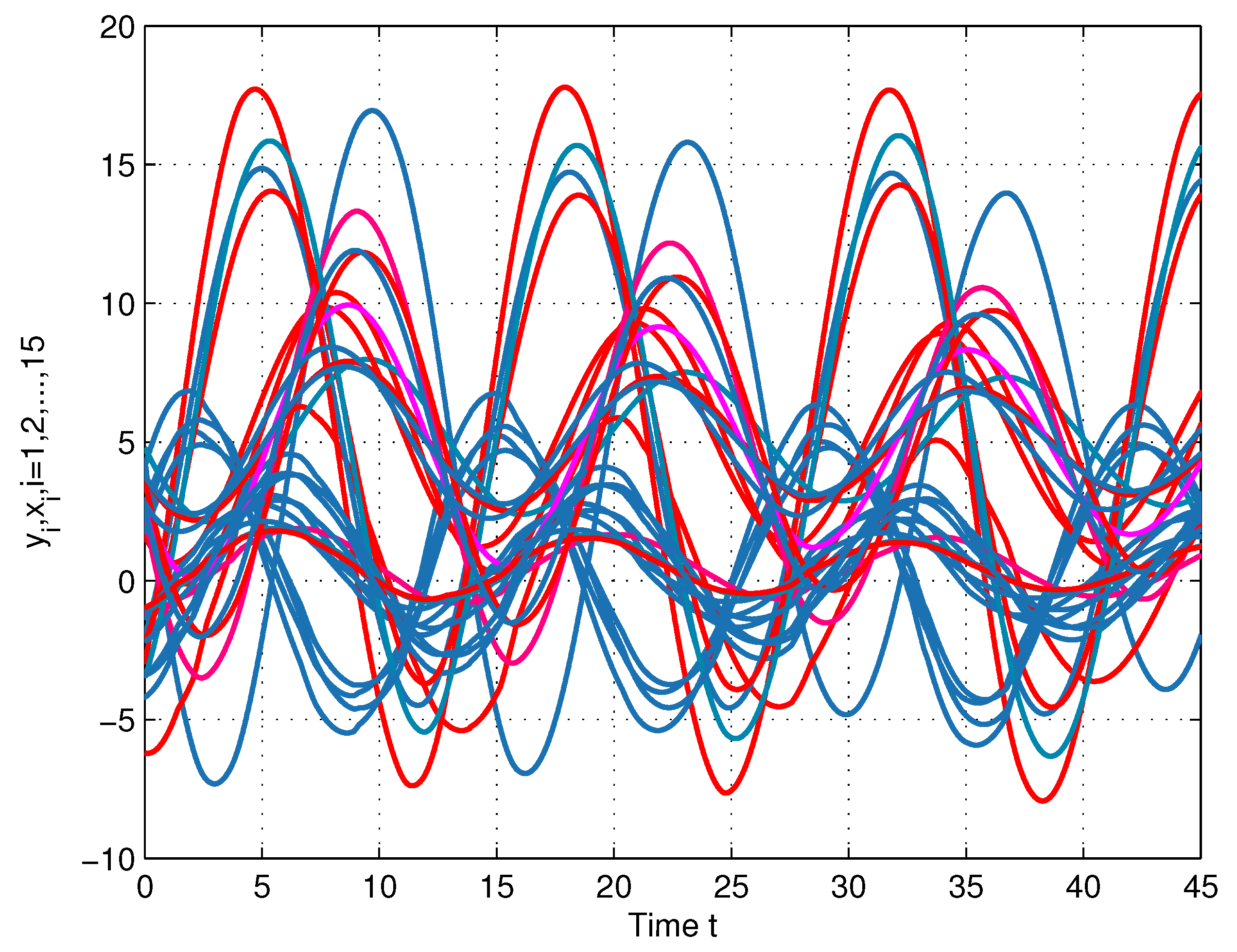
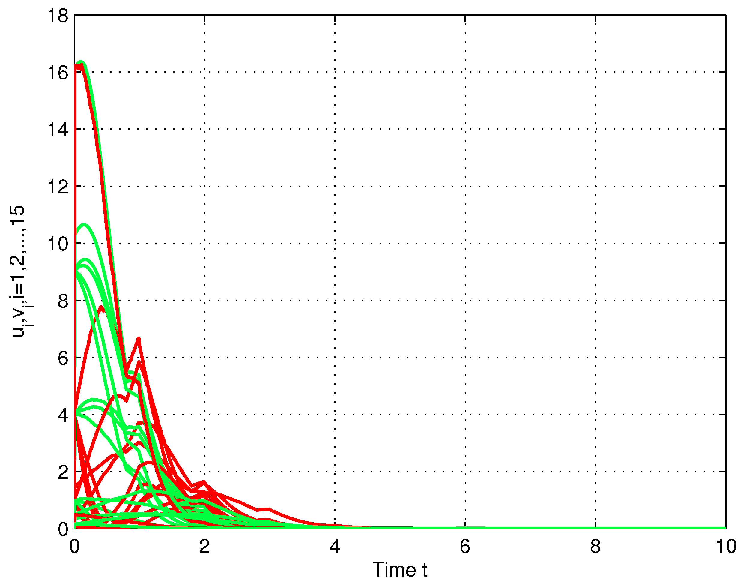
4. Numerical Simulations

This section will provide some numerical simulations to show the effectiveness of the obtained theoretical results.

Let $r_t$ be a Markovian chain taking values in $S=\{1,2\}$; consider the following INNs with 15 vertexes:

$$\left\{\begin{array}{cc}\hfill {\dot{y}}_i(t)=& x_i(t)-{\iota }_i{y}_i(t),\hfill \\ \hfill {\dot{x}}_i(t)=& -\left({\beta }_i(r_t)-{\iota }_i\right)x_i(t)+\left({\iota }_i{\beta }_i(r_t)-{\iota }_i^2-{\alpha }_i(r_t)\right)y_i(t)+\sum _{j=1}^{15}{a}_{ij}(r_t)f_j(y_j(t))\hfill \\ & +\sum _{j=1}^{15}{b}_{ij}(r_t)f_j(y_j(t-{\tau }_1(t))+\sum _{j=1}^{15}{d}_{ij}(r_t){\int }_{t-{\tau }_2(t)}^t{f}_j(y_j(s))\mathrm{d}s+J_i(r_t),\hfill \end{array}\right.$$

(19)

where ${\iota }_i=0.1$, ${\beta }_i(1)=0.01$, ${\beta }_i(2)=0.02$, ${\alpha }_i(1)=0.2$, ${\alpha }_i(2)=0.3$, $J_i(1)=1$, $J_i(2)=1.6$, $i=1,2,\dots ,15$. Let function $f_j(y_j)=0.1tanh(y_j)$, $j=1,2,\dots ,15$, ${\tau }_1(t)=0.2|cost|$ and ${\tau }_2(t)=0.1{sin}^{2}t$. Then one has ${\pi }_j=0.1$, ${\tau }_1=0.2$, ${\tau }_2=0.1$.

We regard system (19) as a drive system; the controlled response system is described as:

$$\left\{\begin{array}{cc}\hfill {\dot{\overline{u}}}_i(t)=& {\overline{v}}_i(t)-{\iota }_i{\overline{u}}_i(t)+u_{i1}(t)+g_{i1}(u_i(t),r_t)\dot{B}(t),\hfill \\ \hfill {\dot{\overline{v}}}_i(t)=& -\left({\beta }_i(r_t)-{\iota }_i\right){\overline{v}}_i(t)+\left({\iota }_i{\beta }_i(r_t)-{\iota }_i^2-{\alpha }_i(r_t)\right){\overline{u}}_i(t)+\sum _{j=1}^{15}{a}_{ij}(r_t)f_j({\overline{u}}_j(t))+u_{i2}(t)\hfill \\ & +\sum _{j=1}^{15}{b}_{ij}(r_t)f_j({\overline{u}}_j(t-{\tau }_1(t))+\sum _{j=1}^{15}{d}_{ij}(r_t){\int }_{t-{\tau }_2(t)}^t{f}_j({\overline{u}}_j(s)\mathrm{d}s+J_i(r_t)\hfill \\ & +g_{i2}(v_i(t),r_t)\dot{B}(t),\hfill \end{array}\right.$$

(20)

where $i=1,2,\dots ,15$, $g_{i1}(u_i(t),1)=0.01sin(u_i(t))$, $g_{i1}(u_i(t),2)=0.021u_i(t)$, $g_{i2}(v_i(t),1)=0.02v_i(t)$, $g_{i2}(v_i(t),2)=0.03sin(v_i(t))$. The coupled strengths are given as

$$\begin{array}{c}{a}_{21}^{(1)}=0.14,a_{32}^{(1)}=0.1,a_{43}^{(1)}=0.2,a_{65}^{(1)}=0.4,b_{1,12}^{(1)}=0.3,b_{2,12}^{(1)}=0.5,b_{13,4}^{(1)}=0.2,d_{75}^{(1)}=0.4,\hfill \\ d_{87}^{(1)}=0.2,d_{10,9}^{(1)}=0.4,d_{12,11}^{(1)}=0.1,d_{14,5}^{(1)}=0.1,d_{15,6}^{(1)}=0.5,a_{32}^{(2)}=0.3,a_{54}^{(2)}=0.3,a_{76}^{(2)}=0.5,\hfill \\ a_{11,1}^{(2)}=0.2,a_{13,2}^{(2)}=0.4,b_{39}^{(2)}=0.3,b_{94}^{(2)}=0.3,b_{14,13}^{(2)}=0.1,d_{91}^{(2)}=0.4,d_{14,6}^{(2)}=0.06,d_{15,7}^{(2)}=0.3,\hfill \end{array}$$

and other weights are 0. A sketch map of digraphs $(G,{(k_{ij}(1))}_{15\times 15})$ and $(G,{(k_{ij}(2))}_{15\times 15})$ are shown in Figure 2. Then, by the direct calculation, we determine that digraph $(G,{(k_{ij})}_{15\times 15})$ is strongly connected, which can also be seen from Figure 3.

Further, let $p_i^{(1)}=2$, $p_i^{(2)}=2.1$; one can derive that $\theta =0.0672$, $\gamma =0.0063$, ${\mathsf{\Xi }}_i=1.131$, and $i=1,2,\dots ,15$. The on–off adaptive controllers are $u_{i1}(t)=-M_i(t)u_i(t)$ and $u_{i2}(t)=-M_i(t)v_i(t)$, and the adaptive law $M_i(t)$ is defined as

$${\dot{M}}_i(t)=\left\{\begin{array}{cc}{\xi }_{i}exp\left\{{\kappa }_{i}t\right\}\left(|u_i{(t)|}^2+{|v_i(t)|}^2\right),\hfill & \hfill t\in [t_n,s_n],\\ 0,\hfill & t\in (s_n,t_{n+1}),\hfill \end{array}\right.$$

(21)

where ${\xi }_i=0.1$, ${\kappa }_i^{(1)}=0.7$, $i=1,2,\dots ,15$, $t_n=n+0.8$. Moreover, take $M_i=1$ and ${\widehat{\kappa }}_i=1.9$, $i=1,2,\dots ,15$. Then, by simple calculation, it holds that

$$\begin{array}{c}\hfill 2M_i-{\mathsf{\Xi }}_i-{\kappa }_i>0,{\widehat{\kappa }}_i-{\kappa }_i-{\mathsf{\Xi }}_i>0,i=1,2,\dots ,15.\end{array}$$

Furthermore, we have ${\kappa }_1=0.7$, ${\kappa }_2=1.2$, and $\epsilon =0.63$ is the solution of $\epsilon -{\kappa }_1+\theta exp\left\{\epsilon {\tau }_1\right\}-\frac{\gamma }{\epsilon }+\frac{\gamma }{\epsilon }exp\left\{\epsilon {\tau }_2\right\}=0$. Obviously, ${\kappa }_1>\theta +\gamma {\tau }_2$ and $\epsilon -({\kappa }_1+{\kappa }_2)\mathsf{\Delta }>0$ hold. It follows from Theorem 2 that the exponential synchronization for drive-response systems (19) and (20) are ensured under aperiodically on–off adaptive control with adaptive law (21). The state trajectories of systems (19) and (20) are given in Figure 4 and Figure 5. Moreover, Figure 6 presented the mean square trajectories of the error system under aperiodically on–off adaptive control with adaptive law (21). These numerical simulations also provide additional confirmation of the results.

5. Conclusions

In this paper, we considered the exponential synchronization of Markov switching inertial neural networks with mixed delays via aperiodically on–off adaptive control. Combined with the Lyapunov method and graph theory as well as the differential inequalities technique, some novel synchronization criteria were established. These criteria principally depend on an on–off controller, Markov switching, and all of the time delay information, and they extend the existing work to a certain extent. Some numerical simulations were provided to show the effectiveness of the obtained theoretical results. Some directions for future research would be to enhance the application scope of the proposed method by studying multi-link topology structures, impulsive models [33], etc.

References

1. Arbi, A.; Cao, J.; Alsaedi, A. Improved synchronization analysis of competitive neural networks with time-varying delays. Nonlinear Anal. Model. Control. 2018, 23, 82–107. [Google Scholar] [CrossRef]
2. Lu, J.; Ho, D.; Cao, J. Exponential synchronization of linearly coupled neural networks with impulsive disturbances. IEEE Trans. Neural Netw. Learn. Syst. 2011, 22, 329–335. [Google Scholar] [CrossRef] [PubMed] [Green Version]
3. Arbi, A.; Tahri, N. New results on time scales of pseudo Weyl almost periodic solution of delayed QVSICNNs. Comput. Appl. Math. 2022, 41, 293. [Google Scholar] [CrossRef]
4. Babcock, K.; Westervelt, R. Dynamics of simple electronic neural networks. Physica D 1987, 28, 305–316. [Google Scholar] [CrossRef]
5. Angelaki, D.E.; Correia, M.J. Models of membrane resonance in pigeon semicircular canal type II hair cells. Biol. Cybern. 1991, 65, 1–10. [Google Scholar] [CrossRef] [PubMed]
6. Koch, C. Cable theory in neurons with active, linearized membrane. Biol. Cybern. 1984, 50, 15–33. [Google Scholar] [CrossRef]
7. Arbi, A.; Tahri, N. Almost anti-periodic solution of inertial neural networks model on time scales. In Proceedings of the 2021 International Conference on Physics, Computing and Mathematical (ICPCM2021), Xiamen, China, 29–30 December 2022; MATEC Web of Conferences. Volume 355, p. 02006. [Google Scholar]
8. Arbi, A.; Tahri, N. Stability analysis of inertial neural networks: A case of almost anti-periodic environment. Math. Methods Appl. Sci. 2022, 45, 10476–10490. [Google Scholar] [CrossRef]
9. Lakshmanan, S.; Prakash, M.; Lim, C.; Rakkiyappan, R.; Balasubramaniam, P.; Nahavandi, S. Synchronization of an inertial neural network with time-varying delays and its application to secure communication. IEEE Trans. Neural Netw. Learn. Syst. 2018, 29, 195–207. [Google Scholar] [CrossRef]
10. Hoppensteadt, F.C.; Izhikevich, E.M. Pattern recognition via synchronization in phase-locked loop neural networks. IEEE Trans. Neural Netw. 2010, 11, 734–738. [Google Scholar] [CrossRef] [PubMed] [Green Version]
11. Tang, Z.; Feng, J.; Zhao, Y. Global synchronization of nonlinear coupled complex dynamical networks with information exchanges at discrete-time. Neurocomputing 2015, 151, 1486–1494. [Google Scholar] [CrossRef]
12. Li, X.; Li, X.T.; Hu, C. Some new results on stability and synchronization for delayed inertial neural networks based on non-reduced order method. Neural Netw. 2017, 96, 91–100. [Google Scholar] [CrossRef]
13. Li, X.; Huang, T. Adaptive synchronization for fuzzy inertial complex-valued neural networks with state-dependent coefficients and mixed delays. Fuzzy Sets Syst. 2021, 411, 174–189. [Google Scholar] [CrossRef]
14. Zhang, Z.; Cao, J. Finite-Time synchronization for fuzzy inertial neural networks by maximum value approach. IEEE Trans. Fuzzy Syst. 2022, 30, 1436–1446. [Google Scholar] [CrossRef]
15. Lakshmanan, S.; Prakash, M.; Rakkiyappan, R.; Joo, Y. Adaptive synchronization of reaction-diffusion neural networks and its application to secure communication. IEEE Trans. Cybern. 2020, 50, 911–922. [Google Scholar]
16. Wang, Y.; Ding, S.; Li, R. Master-slave synchronization of neural networks via event-triggered dynamic controller. Neurocomputing 2021, 419, 215–223. [Google Scholar] [CrossRef]
17. Udhayakumar, K.; Shanmugasundaram, S.; Kashkynbayev, A.; Janani, K.; Rakkiyappan, R. Saturated and asymmetric saturated impulsive control synchronization of coupled delayed inertial neural networks with time-varying delays. Appl. Math. Model. 2023, 113, 528–544. [Google Scholar] [CrossRef]
18. Liu, X.; Chen, Z.; Zhou, L. Synchronization of coupled reaction-diffusion neural networks with hybrid coupling via aperiodically intermittent pinning control. J. Frankl. Inst. 2017, 354, 7053–7076. [Google Scholar] [CrossRef]
19. Wang, P.; Jin, W.; Su, H. Synchronization of coupled stochastic complex-valued dynamical networks with time-varying delays via aperiodically intermittentadaptive control. Chaos 2018, 28, 043114. [Google Scholar] [CrossRef]
20. Wang, P.; Zou, W.; Su, H.; Feng, J. Exponential synchronization of complex-valued delayed coupled systems on networks with aperiodically on-off coupling. Neurocomputing 2019, 369, 155–165. [Google Scholar] [CrossRef]
21. Chen, L.; Qiu, C.; Huang, H. Synchronization with on-off coupling: Role of time scales in network dynamics. Phys. Rev. E 2016, 79, 045101. [Google Scholar] [CrossRef] [PubMed]
22. Wang, G.; Shen, Y.; Yin, Q. Synchronization analysis of coupled stochastic neural networks with on-off coupling and time-delay. Neural Process. Lett. 2015, 42, 501–515. [Google Scholar] [CrossRef]
23. Li, H.; Fang, J.; Li, X.; Rutkowski, L.; Huang, T. Event-triggered synchronization of multiple discrete-time Markovian jump memristor-based neural networks with mixed mode-dependent delays. IEEE Trans. Circuits Syst. I 2022, 66, 2095–2107. [Google Scholar] [CrossRef]
24. Wang, C.; Zhao, X.; Wang, Y. Finite-time stochastic synchronization of fuzzy bi-directional associative memory neural networks with Markovian switching and mixed time delays via intermittent quantized control. AIMS Math. 2023, 8, 4098–4125. [Google Scholar] [CrossRef]
25. Chen, C.; Li, L.; Peng, H.; Yang, Y. Fixed-time synchronization of inertial memristor-based neural networks with discrete delay. Neural Netw. 2019, 109, 81–89. [Google Scholar] [CrossRef] [PubMed]
26. Feng, Y.; Xiong, X.; Tang, R.; Yang, X. Exponential synchronization of inertial neural networks with mixed delays via quantized pinning control. Neurocomputing 2018, 310, 165–171. [Google Scholar] [CrossRef]
27. Prakash, M.; Balasubramaniam, P.; Lakshmanan, S. Synchronization of Markovian jumping inertial neural networks and its applications in image encryption. Neural Netw. 2016, 83, 86–93. [Google Scholar] [CrossRef] [PubMed]
28. Tang, Q.; Jian, J. Exponential synchronization of inertial neural networks with mixed time-varying delays via periodically intermittent control. Neurocomputing 2019, 338, 181–190. [Google Scholar] [CrossRef]
29. Wan, P.; Sun, D.; Chen, D.; Zhao, M.; Zheng, L. Exponential synchronization of inertial reaction-diffusion coupled neural networks with proportional delay via periodically intermittent control. Neurocomputing 2019, 356, 195–205. [Google Scholar] [CrossRef]
30. Li, M.Y.; Shuai, Z. Global-stability problem for coupled systems of differential equations on networks. J. Differ. Equ. 2010, 248, 1–20. [Google Scholar] [CrossRef] [Green Version]
31. Feng, J.; Li, Y.; Zhang, Y.; Xu, C. Stabilization of multi-link delayed neutral-type complex networks with jump diffusion via aperiodically intermittent control. Chaos Soliton. Fractal. 2023, 166, 112947. [Google Scholar] [CrossRef]
32. Guo, B.; Xiao, Y.; Zhang, C. Graph-theoretic approach to exponential synchronization of coupled systems on networks with mixed time-varying delays. J. Frankl. Inst. 2017, 354, 5067–5090. [Google Scholar] [CrossRef]
33. Zhang, T.; Xiong, L. Periodic motion for impulsive fractional functional differential equations with piecewise Caputo derivative. Appl. Math. Lett. 2020, 101, 106072. [Google Scholar] [CrossRef]
Figure 1. Example of a digraph with 5 vertexes.
Mathematics 11 02906 g001
Figure 2. Sketch map of digraphs ( G , ( k i j ( 1 ) ) 15 × 15 ) and ( G , ( k i j ( 2 ) ) 15 × 15 ) . The left is state 1, while the right is state 2.
Mathematics 11 02906 g002
Figure 3. Sketch map of digraph ( G , ( k i j ) 15 × 15 ) , where dotted lines and solid lines represents the connection strengths.
Mathematics 11 02906 g003
Figure 4. The state trajectories of system (19).
Mathematics 11 02906 g004
Figure 5. The state trajectories of system (20).
Mathematics 11 02906 g005
Figure 6. The mean square trajectories of error system under aperiodically on–off adaptive control with adaptive law (21).
Mathematics 11 02906 g006
Disclaimer/Publisher’s Note: The statements, opinions and data contained in all publications are solely those of the individual author(s) and contributor(s) and not of MDPI and/or the editor(s). MDPI and/or the editor(s) disclaim responsibility for any injury to people or property resulting from any ideas, methods, instructions or products referred to in the content.