Abstract
Edge embedding is a technique for constructing low-dimensional feature vectors of edges in heterogeneous graphs, which are also called heterogeneous information networks (HINs). However, edge embedding research is still in its early stages, and few well-developed models exist. Moreover, existing models often learn features on the edge graph, which is much larger than the original network, resulting in slower speed and inaccurate performance. To address these issues, a multi-view learning-based fast edge embedding model is developed for HINs in this paper, called MVFEE. Based on the “divide and conquer” strategy, our model divides the global feature learning into multiple separate local intra-view features learning and inter-view features learning processes. More specifically, each vertex type in the edge graph (each edge type in HIN) is first treated as a view, and a private skip-gram model is used to rapidly learn the intra-view features. Then, a cross-view learning strategy is designed to further learn the inter-view features between two views. Finally, a multi-head attention mechanism is used to aggregate these local features to generate accurate global features of each edge. Extensive experiments on four datasets and three network analysis tasks show the advantages of our model.
MSC:
05C82
1. Introduction
Heterogeneous graphs, which are also called heterogeneous information networks (HINs) have received significant attention in various real-world applications due to their ability to model complex real-world relationships more effectively than homogeneous networks [,,,]. However, the high dimensionality of HINs makes them unsuitable as direct input into network analysis tasks [,,]. To overcome this challenge, heterogeneous information network embedding techniques have been proposed to convert HINs into low-dimensional feature vectors [,,]. These low-dimensional vectors as features of HINs can speed up network analysis tasks and enhance their performance. Heterogeneous information network embedding has shown great promise in multiple network analysis tasks [], such as node classification, node clustering, and link prediction. As HINs become increasingly large and complex, researchers are actively working to develop more effective embedding techniques to support further advances in the field.
Most existing heterogeneous information network (HIN) embedding models focus on generating low-dimensional feature vectors for each node, which are suitable for node-based network analysis tasks, such as node classification and node clustering. For example, HIN2vec [] learns the embedding for different types of nodes and their relationships based on meta-paths. HAN [] uses an attention mechanism to capture rich semantic information of nodes, which is also a heterogeneous information network embedding model. However, edge-based analysis tasks, including edge classification, edge clustering, and link prediction, cannot be neglected. Edge-based tasks require a low-dimensional feature vector of each edge as input. Therefore, recent research has focused on developing edge embedding techniques that learn edge features from complex networks.
The existing edge embedding models can be simply classified into two categories. (1) The first category is indirect edge embedding models. These models do not directly generate the low-dimensional features of edges in the network. Instead, they derive the feature vectors of edges using the Hadamard product of the feature vectors of the two end nodes connected to the edges. For example, the node2vec model [] indirectly obtains the edge features by applying the average or Hadamard product on the embedding of the two end nodes connected to the corresponding edge. However, node2vec is solely suitable for homogeneous information networks, as it treats all nodes and edges as a single type. Similarly, AspEm [] treats a heterogeneous information network as multiple views to address the misalignment problem between different edge types. HEER [] uses edge representations and heterogeneous metrics to address semantic incompatibilities in HINs. Both of them generate the edge embedding by performing the Hadamard product on the embedding of two end nodes. While indirect models are highly efficient, they often sacrifice the accuracy of edge embedding. (2) The second category is direct edge embedding models. These models usually first convert a HIN into its edge graph, where each edge in the original network is converted into a vertex in the edge graph. Then, different neural networks [,,,,,] are used to learn the vertex features of the edge graph, which means learning the edge features of the original network. For example, the Edge2vec model [] first converts each edge in the original network into a vertex in the edge graph. Then, it uses a random walk strategy on the edge graph to generate a vertex sequence and applies a skip-gram model to learn the embedding of these vertexes. Gl2vec [] uses the acquired edge information of the constructed edge graph and feeds it back into the original network to enhance the quality of the learned embedding. These direct models outperform indirect models in edge-based network analysis tasks. CensNet [] is a deep model that uses GCN to obtain vertex embeddings from the edge graph of the original network. This approach allows CensNet to extract features at a deeper level than shallow models, at the cost of increased computational time. And most direct models typically transform the original network into a larger edge graph, which is a time-consuming process. In addition, most direct models are designed for homogeneous information networks and cannot be easily adapted to the heterogeneity of heterogeneous information networks.
In summary, the edge embedding for HINs is still in its early stage and there are few mature models. In addition, with the continuous growth in size and complexity of HINs, edge embedding for HINs still faces two challenges.
- Difficult to extract complex network features. With the development of big data technology, HINs have grown increasingly complex. As a result, the latent features they contain are becoming more complex and diverse, making them more difficult to extract. However, the existing indirect embedding models are unable to learn edges directly, causing a significant loss of edge information. The direct edge models are generally designed for homogeneous information networks, resulting in poor feature separation and low feature extraction accuracy when applied to heterogeneous information networks.
- Difficult to balance speed and performance. As the size of HINs increases, the network analysis tasks become more time-sensitive, requiring an embedding model with high speed and performance. However, the existing edge embedding models usually convert the original network into a larger edge graph. Moreover, when using a deep model to enhance nonlinear feature extraction, the time complexity of the model increases. Therefore, edge embedding models with high speed and performance must be further researched.
The motivation of this paper is to develop a fast and high-performing edge embedding model for HINs to overcome the above-mentioned challenges. To obtain high speed, the shallow model is used instead of the deep model to ensure the efficiency of edge embedding and cope with the large-scale HINs. To ensure accuracy, the edge graph of HINs is divided into multiple views, and the global features of an edge are divided into local intra-view features and local inter-view features. In this way, each local feature is purer and simpler, and it is more convenient for shallow models to extract accurately. To further speed up, a multi-view learning strategy is used to learn local features in a divide-and-conquer manner. Based on these ideas, a multi-view learning-based fast edge embedding model is proposed for HINs, called MVFEE. The main contributions of this paper are as follows.
- A shallow single-view learning strategy is designed to rapidly learn intra-view features for each view in the edge graph, where each vertex type is considered a separate view;
- A novel shallow cross-view learning strategy is designed to further learn the inter-view features between two views;
- A multi-head graph attention mechanism is used to accurately aggregate local features of multiple views, so as to generate a global edge embedding;
- Extensive experiments on three network analysis tasks and four public datasets show the good performance of our MFVEE model.
2. Definition
In this section, several definitions used in this paper are first introduced.
Definition 1 (Heterogeneous Graph).
Heterogeneous graphs, which are also called heterogeneous information networks (HINs) are complex networks with different types of nodes and edges. A HIN can be defined as G = (V, E), where V denotes the set of nodes and E denotes the set of edges. is a mapping function between nodes, edges, and their corresponding types. For each node ni ∈ V, there is a (ni) = Tk ∈ T where T denotes the set of node types. For each edge li ∈ E, there is a (li) = Rs ∈ R where R denotes the set of edge types. In addition, the |T| + |R| ≥ 2 where |*| is the number of elements in the set *.
Definition 2 (Edge Graph).
In an edge graph, also known as a line graph [], each vertex is an edge of the original network, and a link between two vertexes is constructed when the corresponding two edges in the original network share a common node. An edge graph of a HIN can be defined as G′ = (V′, E′), where V′ denotes the set of vertexes and E′ denotes the set of links. For the original network G = (V, E), each edge li ∈ E is a vertex v(li) ∈ V′ in the edge graph. And when two edges li ∈ E and lj ∈ E share a common node no, a link e(v(li), v(lj)) ∈ E′ is connected in the edge graph. The number of vertexes in G′ is usually greater than the number of nodes M in G. The number of links in G′ is also usually greater than the number of edges in G. The edge graph can better present the adjacency of edges in the original network and can help us to highlight the edge features.
Definition 3 (Heterogeneous Graph Edge embedding).
Edge embedding in heterogeneous graphs refers to mapping edges from the high-dimensional network space into a low-dimensional vector space. In this paper, a heterogeneous graph G = (V, E) is first transformed into its edge graph G′ = (V′, E′), and a mapping function f: V′ → 1×d is designed to perform the edge embedding on the G′ where d denotes the dimensional of the embedding. After mapping, each edge li can obtain a low-dimensional feature vector xi ∈ 1×d which can preserve its features in the original network.
3. Framework
3.1. Overview
As the era of big data advents, real-world HINs are expanding and becoming more heterogeneous. That is to say, the HINs become harder to accurately and efficiently extract features because of their additional types of nodes and edges, more diverse features, and more coupled correlations between features. Moreover, with the rapid development of network science, there is an increasing number of edge-based downstream network analysis tasks, such as link prediction, association analysis, relationship clustering, and so on. These edge-based downstream tasks call for more real-time and more accurate edge embedding models. To meet these requirements, this paper tries to build a multi-view learning-based fast edge embedding model, called MVFEE, to accurately and quickly capture the embedding feature of each edge. To obtain a better edge embedding, the model first transformed an original heterogeneous information network into its edge graph. To reduce the difficulty of embedding and extracting features more accurately, our model treats each vertex type (or edge type in the original network) as a separate view and divides the edge graph into multiple views. This division allows the features of one edge to be categorized into intra-view local features and inter-view local features. Additionally, we use a multi-view learning strategy to help the model learn features more efficiently in a divide and conquer approach. To further optimize speed, we use shallow networks instead of deep ones to quickly learn each sub-feature.
The framework of our MVFEE model is shown in Figure 1. The MVFEE model consists of four components. (1) Edge graph construction. This component is responsible for transforming a HIN into its edge graph, as shown in Figure 1a. In the edge graph, one edge of the original network is transformed into a vertex and a new link is built if two vertexes (two edges of the original network) are adjacent in the original HIN. Based on the edge graph, we can better learn the features of each edge in the original HIN. (2) Single-view learning for intra-view features. In the edge graph, each vertex type (an edge type of the original network) is seen as a view, as shown in Figure 1b. A private shallow skip-gram model is used to quickly learn the proximity of multiple vertexes within this view (multiple edges of the original network), so as to capture the intra-view local features. (3) Cross-view learning for inter-view features. In the edge graph, each link type is seen as the semantic similarity between two views, as shown in Figure 1c. A novel shallow cross-view learning strategy is designed to rapidly learn the inter-view local features of two views, and the inter-view features are fused to the learned intra-view features. (4) Multi-view Feature aggregation. The multi-head graph attention network, which is shown in Figure 1d, is further used to aggregate the local features of multiple views and then generate the global features for each edge.
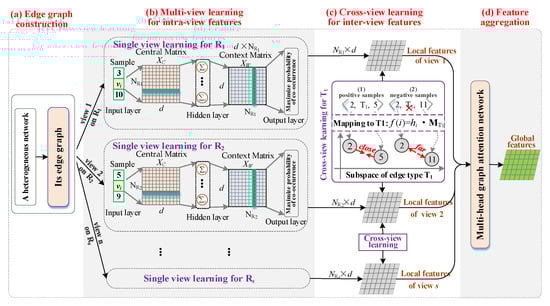
Figure 1.
The framework of the MVFEE model.
3.2. Edge Graph Construction
In a heterogeneous information network (HIN), an edge may be related to multiple nodes and edges with different types. Due to heterogeneity, feature associations between edges of the same type and the associations between edges of different types need to be studied separately. Therefore, the features of an edge consist not only of its closeness (intra-view proximity) to adjacent edges of the same type but also its semantic similarity (inter-view similarity) with adjacent edges of different types. However, it is difficult to judge whether two edges are directly adjacent or high-order adjacent in the HIN. For this reason, transforming a HIN into its edge graph can improve the learning of edge embeddings.
Figure 2 shows the process of constructing the edge graph of a HIN. First, each edge in the original HIN is transformed into a vertex in the edge graph, and the type of the edge is changed to the type of the vertex. For example, in Figure 2, edge 2 in the HIN is transformed into vertex 2 in the edge graph, and the type R1 of edge 2 in the HIN is the type of vertex 2 in the edge graph. Second, a link is built when two vertexes (two edges of the original network) are adjacent in the original HIN. In other words, if the two edges in the original network are adjacent, there is a common node between the two edges, and then a new link is created between the two vertexes in the edge graph. Moreover, the type of the new link in the edge graph is the type of the common node in the original network. When both vertexes and links are generated, the edge graph of the original HIN is also constructed.
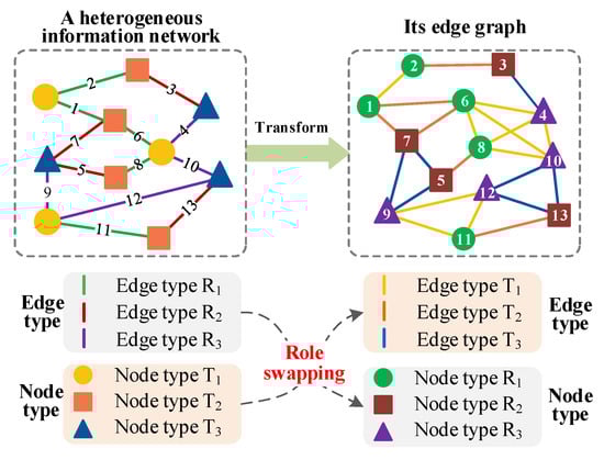
Figure 2.
The construction process of the edge graph.
It is easy to find some characteristics of the edge graph. (1) The edge graph is a heterogeneous graph as well, consisting of multiple different types of vertexes and links. (2) The edge types in the original network are the same as the vertex types in the edge graph, and the node types in the original network are the same as the link types in the edge graph. That is to say, node and edge types are exchanged between the original network and its edge graph. (3) The number of vertexes in the edge graph is the same as that of the edges in the original network, while the number of links in the edge graph is much larger than that of the nodes in the original network.
3.3. Single-View Learning for Intra-View Features
The first feature of an edge is its proximity to multiple edges of the same type in the original heterogeneous information network, which includes both 1-order proximity (i.e., direct adjacency) and higher-order proximity (i.e., multi-hop adjacency). To better capture the adjacent relationships between edges, the edge graph of the original network is used as the learning object. In the edge graph, each vertex type (R1~Rs) is treated as a separate view. In view R1, all R1-Type vertexes in the edge graph are assigned to this view. To quickly capture the first feature, a multi-view learning strategy is used based on the concept of “divide and conquer”. Specifically, a private skip-gram model is used for intra-view feature learning in each view to speed up the learning of one-order and higher-order proximity. After learning the intra-view features, a low-dimensional feature matrix with a size of × d is generated for each view, where is the number of Ri-type vertexes in the edge graph. It should be noted that + … + NRs = N, where N is the total number of vertexes in the edge graph. Taking the R1-type view as an example, the process of intra-view features learning is shown in Figure 3.
- Sampling. To capture the one-order and high-order intra-view neighbors, we generate some training samples for the skip-gram model. First, an R1-type vertex is randomly chosen from the edge graph as the starting vertex, and the random walk with a restart rate of 30% is repeatedly performed to obtain a vertex sequence of length L. Next, all R1-type vertexes are further selected from the generated walk sequence as a candidate subsequence. Then, this candidate subsequence is divided into several samples, and each sample consists of Win adjacent vertexes. The Win is the preset hyper-parameter, representing the window size of a sample. According to Section 4.6, the default value of Win in this stage is set as three. For example, the first to the Win-th in the subsequence is the first sample, and the second to the (Win + 1)-th is the second sample. When the window size Win is three, a sample <5, vi, 6> is generated where vi is the central vertex and the other vertexes are its contextual neighbors or positive vertexes. Additionally, the remaining vertexes 10 and 12 in the candidate subsequence are the negative vertexes. In this way, each sample includes both one-order and high-order proximity. Finally, this process is repeated until every R1-type vertex in the edge graph has been used as a starting vertex for a random walk.
- Input. The generated samples are input. In this paper, each view has a private skip-gram model consisting of a simple three-layer structure: an input layer, a hidden layer, and an output layer, as shown in Figure 3a. There is a central matrix XC ∈ N×d between the input layer and the hidden layer, a context matrix XW ∈ d×N between the hidden layer and the output layer where two matrices are randomly initialized, is the number of R1-type vertexes, and d is the dimension of the edge embedding.
- Learning process. First, a sample <5, vi, 6> is divided into the central vertex vi and contextual neighbors [,]. Second, the one-hot code of the central vertex vi is used as input of the skip-gram model to calculate the code of the hidden layer and defined as:where onehot() is the function to calculate the one-hot code, the size of the one-hot code for vi is 1 × , and the size of hi is 1 × d.
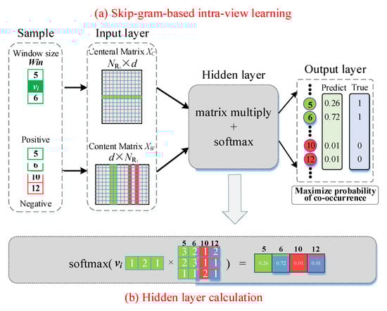
Figure 3.
Single-view learning for intra-view features.
Then, the code of the hidden layer is decoded as output and defined as:
where oi is a similarity vector between the central vertex vi and other R1-type vertexes, the size of oi is 1 × . In the oi, the k-th element represents the similarity between vertex vk and central vertex vi.
Finally, the softmax function is used to regularize the similarity between the central vertex vi and other R1-type vertexes and defined as:
where oi (j) is the j-th element in the oi, representing the similarity between the central vertex vi and the neighbor vi.
After regularization, the value of each element in Si is in the range of [0, 1]. Moreover, when Si (j) is close to one, it means that the central vertex vi and the vertex vj are one-order or high-order neighbors. In contrast, the central vertex vi and the vertex vj are not neighbors. Taking a sample <5, vi, 6> as an example, vertexes 5 and 6 are the neighbors for vertex vi. In Si, Si (5) and Si (6) should converge to one, and Si (10) and Si (12) should converge to zero, as shown on the right of Figure 3a. Furthermore, the concept of “Maximize probability of co-occurrence” depicted in Figure 1b and the right side of Figure 3a pertains to transforming the similarity values of positive samples with the central vertex to one and adjusting the similarity values of negative samples to zero.
- Loss Function. We aim to learn the proximity between vertexes in view R1 by adjusting the similarity between the central vertex vi and its context neighbors. Therefore, a sample is divided into the central vertex and its contextual neighbors. The contextual neighbors are the positive training samples for the central vertex. And the other R1-type vertexes are the negative training samples for the central vertex. Usually, the number of negative samples is much greater than the number of positive samples. To speed up training, the negative sampling strategy is used to randomly select M samples from all negative samples as the final negative samples. For a positive sample, the similarity to the central vertex vi should converge to one. For a negative sample, the similarity to the central vertex vi should converge to 0. Therefore, the loss function is defined as follows.where Neg (vi) represents the negative samples of the central vertex vi, Pos (vi) represents its positive samples, and Si (j) represents the j-th element of Si.
After the training, the central vertex feature matrix XC is the final intra-view features matrix of the R1-type view.
3.4. Edge Graph Construction
The second feature of one edge is the semantic similarity of multiple edges with different types in the original heterogeneous information network, which also contains the one-order similarity (i.e., direct adjacency) and higher-order similarity (i.e., multi-hop adjacency). In the edge graph, the semantic similarity of two edges with different types in the original network is the semantic similarity of two corresponding vertexes of different types. That is to say, if there is a link between two vertexes with different types in the edge graph, there is a semantic similarity between them. Moreover, multiple links of the same type have the same semantic similarity. Since each vertex belongs to only one view, semantic similarity can be regarded as a local feature of two views. Based on the above ideas, each link type in the edge graph is treated as a semantic subspace where heterogeneous vertexes of two views share the same distribution of semantic similarity. To learn the semantic similarity of each link type, a novel cross-view learning strategy is designed to learn the inter-view local features.
For a link type, cross-view learning is to capture the semantic similarity between two views. That is to say, the inter-view features and the intra-view features are complementary and together constitute the global feature of an edge in the original network. Therefore, the cross-view learning for a link type takes the intra-view features of two views as initial features and updates them. In this way, the inter-view features and the intra-view features can be effectively fused to generate the global features of each view. Taking the link type T1 in the edge graph as an example, the process of cross-view learning is shown in Figure 4.
- Sampling. To capture the one-order and high-order inter-view neighbors, we perform the inter-view sampling procedure. First, a T1-type link is randomly selected from the edge graph, and a vertex of this edge is randomly selected as the starting vertex. From the starting vertex, the random walk with a restart rate of 30% is repeatedly performed to obtain a vertex sequence of length L. Second, all the vertexes related to type T1 (belonging to one of the two end vertex types of type T1) in the vertex sequence are chosen sequentially as the positive subsequence. The remaining vertexes are chosen sequentially as the negative subsequence. Next, the positive subsequence is divided into multiple windows of length Win. The default value of Win in this stage has been set to three based on careful consideration and experimentation in Section 4.6 to ensure optimal performance and achieve the desired results. For example, when the Win is 3, [1,2,5] is a window and [2,5,7] is another window. Any two nodes in a window can constitute a positive sample. So, the window [1,2,5] can be generated as three positive samples <1,T1,2>, <1,T1,5>, and <2,T1,5>. In this way, the generated positive samples may contain one-order or higher-order semantic similarity. For example, if vertex 1 is adjacent to vertex 2, these two vertexes have one-order semantic similarity, otherwise, they have a high-order semantic similarity. Then, according to the same method, a large number of negative samples are generated from the negative subsequence. Finally, the process is repeated until every T1-type link has been treated as a starting place for a random walk. The whole sampling process is shown in Figure 4a.
- Input. The positive samples <vi, T1, vj> and the negative samples <vi, not T1, vo> are the first input. The intra-view features matrices of all views XC~XC are the second input. The projection matrix of the T1-type semantic subspace with size d × d is the fourth input, which is initialized randomly.
- Learning process. Based on the idea that “if a link exists between two vertexes with different types, the coordinates of the two vertexes in the semantic subspace should be close”, the cross-view feature learning of the link type T1 is to project two vertexes with different types into the same semantic subspace, and then pull the coordinates of the two vertexes as close together as possible when the two vertexes are 1-order or high-order neighbors, or push the coordinates of the two vertexes as far away as possible when the two vertexes are not neighbors.
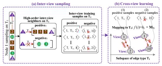
Figure 4.
Cross-view learning for inter-view features.
First, the two vertexes in a sample are mapped to the semantic subspace of T1, and the coordinates of the two vertexes are obtained, respectively, as follows.
where xi ∈ 1×d is the intra-view features vector of vertex vi in XC, xj ∈ 1×d is the intra-view features vector of vertex vj in an XC of corresponding vertex type.
Second, since the coordinates of two vertexes are vectors, the inner product of the two vectors is used to calculate the semantic similarity of two vertexes in the semantic subspace, as follows.
where ● represents the dot product operator.
Then, the sigmoid function is used to regularize the distance between vertexes to obtain a more easily comparable semantic similarity. The sigmoid function and semantic similarity computation of two vertexes are defined as follows.
After regularization, the semantic similarity between two vertexes is quantified into the range of [0, 1]. If two vertexes are one-order order or higher-order semantic neighbors, then the semantic similarity between them should be close to one. Otherwise, the semantic similarity should be close to 0.
- Loss Function: In the learning process, for one positive sample < vi, T1, vj >, vertex vi is pulled close to vertex vj in the T1 semantic subspace, increasing the similarity between them. And for one negative sample <vi, not T1, vo>, vertex vi is pulled far to vertex vo in T1 semantic subspace, decreasing the similarity between them. The similarity loss function is defined as follows.where Pos are all positive samples and Nes are all negative samples.
The final feature matrices and output following training are the intra-view features matrices XC~XC of all views.
3.5. Multi-View Feature Aggregation
After completing the above processes, the embedding vector matrix of each view is generated. However, the final global edge embedding has not yet been established. In addition, since random sampling is used in the above learning processes, the learned embedding vectors of each view may be slightly rough. To address these problems, based on the edge graph topology, a multi-view feature aggregation strategy is designed to use the multi-head graph attention mechanism to aggregate local features, so as to generate the global edge embedding. The whole aggregation process is shown in Figure 5.
- Input: The feature matrices of all views XC~XC are the first input. The adjacency matrix of the edge graph A is the second input.
- Learning process: Taking the attention head F1 in this process as an example.
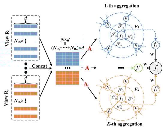
Figure 5.
Multi-view feature aggregation.
First, all the feature matrices XC~XC are spliced into a complete feature matrix , as follows:
where s represents the total number of vertex types in the edge graph, and the concat function is used to splice all the feature matrices to a matrix of size N×d.
Second, the attention head learns the neighborhood information of all vertexes in the feature matrix f based on the edge graph adjacency matrix A. An attention head is initialized to calculate the attention coefficients between two vertex features fi ∈ f and fj ∈ f, as follows:
where concat means to splice fi and fj to a vector of size 1 × 2d and ● represents the dot product operator.
Third, the weights of neighboring vertexes are calculated by the activation function softmax, as follows:
where Neighbors(i) represents the set of all the neighbors of vertex i.
Next, the features of surrounding vertexes of vertex i are aggregated to according to corresponding , as follows:
where U is the parameter matrix that updates the vertex features. In addition, in order to enhance the representation and self-renewal capability of the vertex, our model treats the vertexes themselves as their neighboring vertex. In other words, .
Then, the same program is performed in K attention heads. Linear transformation is employed to compute the final feature vector fi of vertex i as follows:
where k represents the in the k-th attention head, concat means to splice to a matrix of size d × (K × d), and represents the weight matrix.
Finally, all vertexes have aggregated the neighbor information through the above process, and a new feature matrix is obtained.
- Loss Function: In the learning process, the inner product of the vertex features in the obtained feature matrix is used to compute the probability of adjacency between vertexes. And the probability is used to reconstruct edge graph adjacency matrix as follows:where T represents transposition, and N is the number of vertexes, and ● represents the dot product operator.
Then, cross-entropy loss is used to adjust this reconstructed adjacency relationship to make it similar to the real edge graph adjacency matrix A as follows:
where indicates whether vertex i and vertex j are connected (1) or not (0), and indicates the probability whether vertex i and vertex j are connected.
After the training, the obtained feature matrix is the final global edge embedding of the heterogeneous information network.
3.6. Model Training
The training process of our MVFEE model is as follows: (1) The single-view learning process for one view is performed for 10 epochs. In each epoch, the training samples are independently sampled. To speed up the process, single-view learning processes for multiple views are performed in parallel. (2) The cross-view learning for each link type is performed for 10 epochs based on the learned intra-view features. In each epoch, the training samples are also independently sampled for each link type. (3) The single-view learning and the cross-view learning are alternated for two–three rounds. (4) The feature aggregation is performed for five epochs using a six-head graph attention in each epoch.
In the single-view learning process and cross-view learning process, the stochastic gradient descent (SGD) algorithm is used to update parameters with a learning rate of 0.2 and a decay rate of 0.0001. In the multi-view feature aggregation process, the Adam optimizer is used to update parameters with a learning rate of 0.005 and a decay rate of 0.0005.
4. Experiment
4.1. Experimental Setup
- Datasets. Five datasets were used in our experiments, as shown in Table 1. (1) AMiner [] (http://arnetminer.org/aminernetwork (10 March 2023)). The AMiner is a widely used academic graph in the research community for tasks such as paper recommendation, academic network analysis, and citation prediction. The latest version of AMiner contains billions of edges. To simplify this dataset, we have extracted a core set that has four node types and three edge types from it. (2) IMDb (https://datasets.imdbws.com/ (10 March 2023)). IMDb is a widely used online dataset that provides information about movies, TV shows, video games, and other forms of entertainment. It contains a vast collection of structured data about movies, including cast and crew information, plot summaries, user ratings, and other details. To simplify this dataset, we extracted a core set that has four node types and three edge types from it. (3) ACM (https:/www.aminer.org/citation (10 March 2023)). The ACM Citation Network dataset is commonly used for research in bibliometrics and network analysis, as well as for developing machine learning algorithms for citation prediction and recommendation systems. Since we are only interested in papers and their citation relationships, we have extracted a core set consisting of four node types and four edge types. (4) Douban [] (https://www.dropbox.com/s/u2ejjezjk08lz1o/Douban.tar.gz?dl=0 (10 March 2023)). The Douban dataset is a collection of structured data about movies, TV shows, music, books, and other forms of entertainment, along with user ratings, reviews, and other metadata. It contains numerous nodes representing different types of media, including those representing different types of media (movies, TV shows, music, and books), as well as nodes representing users and groups. To simplify the Douban dataset, we extracted a core set comprising four node types and three edge types.
 Table 1. Dataset.
 - Tasks and metrics. Three downstream edge-based network analysis tasks and their corresponding evaluation metrics were selected. (1) Edge classification is the first task. This task predicts the category of an edge based on the previously learned low-dimensional edge embedding vectors. It is common in recent network analysis tasks [,]. We pre-labeled edges in four networks based on their end node labels, and the edge labels are invisible to the model training. Micro-F1 and Macro-F1 are the two widely accepted evaluation metrics, with values between [0 and 1]. Micro-F1 first calculates the precision and recall for each class, and then performs a weighted average of the precision and recall for all classes, without considering class imbalance. Macro-F1 is a metric that calculates F1 values independently for each class, and then performs an arithmetic average of F1 values for all classes, without considering the sample size differences of the classes. (2) Edge clustering is the second task. The task applies a simple K-Means algorithm to divide the edges in a HIN into several disjoint subgroups with a class represented by each subgroup, based on the learned low-dimensional edge embedding vectors. Similar to the edge classification task, edge clustering is also a common network analysis task [,], and the labels of edges in four networks were pre-labeled. We selected NMI (Normalized Mutual Information) as the evaluation metric for this task, with values between [0 and 1]. A higher NMI value indicates that the clustering results are more consistent with the labels, while the opposite indicates that the clustering results are less consistent with the labels. (3) Link prediction is the third task. Link prediction is also a very common task for network analysis [,]. Based on the learned edge embeddings, this task predicts whether an edge exists in the network. If the edge exists, the label of it is set as one. Otherwise, the label is set as 0. We chose ACC (Accuracy) and AUC (Area Under the Curve) as our evaluation metrics for this task, with values between [0 and 1]. ACC measures the correctness of model predictions in link prediction, that is the ratio of the number of correct predictions to the number of all predictions. The AUC metric is the comparison of the similarity values of edges to the similarity values of non-existent edges.
- Baselines. As displayed in Table 2, the node embedding models HIN2vec and HAN, indirect edge embedding models AspEm and HEER, and direct edge embedding models Edge2vec and CensNet were used in the experiments. Among them, HAN and CensNet are deep models, while others are shallow models. By adjusting the default parameters, the best experimental results were obtained for all these algorithms, and the performance of our proposed model MVFEE was compared with these five typical baseline algorithms on the four real-world datasets mentioned above.
Table 2. Baselines.
- Parameters settings. The default parameters used for each algorithm are set as follows, and for each dataset, we fine-tuned the parameters to achieve the best performance based on these default values. (1) HIN2vec. We set the window size to 3, the walk length to 80, and the embedding dimension to 128. The learning rate was set to 0.025, the number of negative samples was set to 5, and the number of iterations was set to 10. (2) HAN. We used four attention heads in each layer and set the embedding dimension to 128. The learning rate was set to 0.005 and the weight decay was set to 0.01. (3) AspEm. We set the number of negative examples to 5, the embedding dimension to 128, and the initial learning rate to 0.025. (4) HEER. We set the embedding dimension to 128, the window size to 3, and the batch size was set to 50. (5) Edge2vec. We set the negative sampling to 500, the embedding dimension to 128, and the learning rate was set to 0.025. (6) CensNet. The dropout was set to 0.5, the initial learning rate was set to 0.01, the embedding dimension to 128, the weight decay was set to 0.0005, and the number of epochs was set to 200.
- Setting. The experimental platform was a PC server equipped with a T4 graphics card. The server has a 12-core Intel Core i7-12700 processor, 128 GB of RAM, and runs on the Ubuntu 20.04 operating system. We programmed the MVFEE algorithm using the PyCharm IDE and the Python programming language. The source code for the other algorithms can be downloaded from URLs in Table 2.
4.2. Edge Classification
The first experimental goal was to take edge classification as the task to evaluate the performance of our MVFEE model and the multi-view feature aggregation strategy. We used Micro-F1 and Macro-F1 metrics to evaluate the performance of these models on selected datasets.
4.2.1. Performance Analysis of Our MVFEE Model
To verify MVFEE’s performance, we selected five typical algorithms as baselines to perform the edge classification task on the AMiner, ACM, and Douban datasets. Moreover, the embedding vectors of the edges were used as the input of edge classification. For HIN2vec and HAN, we obtained the embedding vectors of the edges by taking the Hadamard product of the embedding of the two end-nodes connected by the corresponding edge. As for AspEm and HEER, we used the learned edge embedding as the input for the edge classification task. For Edge2vec, it is designed for homogeneous networks. Thus, we first use multiple meta-paths to extract homogeneous subgraphs from the edge graph. Then, Edge2vec is applied to learn these subgraphs to obtain the embedding vectors of the edges. As for CensNet, it was originally designed for graph embedding. In our experiments, we processed it like Edge2vec to improve its performance.
Figure 6 shows the edge classification accuracy of six algorithms on AMiner, ACM, and Douban, where HIN2vec is represented with gray lines, HAN with red lines, AspEm with blue lines, HEER with green lines, Edge2vec with purple lines, CensNet with yellow lines, and our model MVFEE with cyan lines. And the first row (Figure 6a–c) of the figure corresponds to the Micro-F1 score of the six algorithms, while the second row (Figure 6a′–c′) corresponds to the Macro-F1 score. The Micro-F1 and Macro-F1 scores for the algorithms were 0.61 and 0.37 on average. Further analysis of the results highlights the following observations. (1) Comparing the six models, the MVFEE and Edge2vec models had a better performance on all networks, while HAN performed better than AspEm and HEER, and HIN2vec had the worst performance. (2) Considering different embedding methods, the edge embedding models (MVFEE, Edge2vec, AspEm, and HEER) generally performed better than the node embedding models (HAN and HIN2vec). For example, on the AMiner network, Macro-F1 scores reached 0.8619 for MVFEE and only 0.8265 for HIN2vec. Similarly, on the Douban network, Macro-F1 scores reached 0.2469 for Edge2vec and only 0.2239 for HIN2vec. (3) Focusing on the edge embedding models, the MVFEE outperformed all others on all networks, while Edge2vec performed better than AspEm and HEER. For example, on the ACM network, the Micro-F1 scores for MVFEE (0.6397) and Edge2vec (0.6332) were higher than those of AspEm and HEER, which were 0.6083 and 0.6086, respectively. (4) Considering the depth of the edge embedding models, our shallow MVFEE model performed better than the deep CensNet model on most networks. For example, on the AMiner network, MFVEE achieved a Micro-F1 score of 0.8619, while CensNet only achieved 0.8564. (5) Considering the network density, our MVFEE model showed higher edge classification accuracy on sparser networks (AMiner and ACM) than on denser ones (Douban). For example, the highest Micro-F1 and Macro-F1 scores of MVFEE were only 0.4006 and 0.2536 on the Douban network but could reach 0.6397 and 0.3248 on the ACM network. These findings highlight the effectiveness of edge embedding methods for edge classification tasks, as well as the high performance of our model MVFEE across different networks.
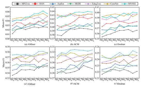
Figure 6.
Performance analysis of multiple algorithms on edge classification.
4.2.2. Performance Analysis of Multi-View Feature Aggregation
The MVFEE model uses a multi-view feature aggregation strategy with a multi-head attention mechanism to generate accurate global edge embedding. We designed a simplified version of this model, named simplified MVFEE, which directly splices embeddings in all views learned by the intra-view learning and inter-view learning strategies without the attention mechanism. To validate the effectiveness of the multi-view feature aggregation strategy, we used simplified MVFEE and MVFEE on four experimental datasets (AMiner, IMDb, ACM, and Douban) for the edge classification task. Then, Micro-F1 and Macro-F1 were selected as evaluation metrics.
As shown in Figure 7a,b, we compared the edge classification accuracy of MVFEE (orange) and simplified MVFEE (blue) on four networks. Our analysis of Figure 7 reveals the following insights. (1) Comparing the two models, the MVFEE model had better performance on all four networks than the simplified MVFEE model, as measured by both Micro-F1 and Macro-F1 scores. For example, the MVFEE model achieved Micro-F1 and Macro-F1 scores of 0.7928 and 0.4728 on the IMDb network, while the simplified MVFEE model only achieved 0.6411 and 0.3519. (2) Focusing on the density of the network, the difference in accuracy between the two models was more pronounced in sparse networks. For example, the Micro-F1 score of the MVFEE was 14.6% higher than the simplified MVFEE model on the AMiner network, while the improvement was only 8.4% on the Douban network. This disparity may be due to greater complexity in interactions between nodes in dense networks, resulting in more complex features at the edge. The attention mechanism in the MVFEE model is better equipped to aggregate these features in sparse networks (AMiner and IMDb) than in denser networks (ACM and Douban).
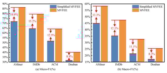
Figure 7.
Performance analysis of multi-view feature aggregation on edge classification.
4.3. Edge Clustering
The second objective of our experiments was to use normalized mutual information (NMI) as an evaluation metric to validate the performance of our MVFEE model and multi-view feature aggregation strategy in the edge clustering task.
4.3.1. Performance Analysis of Our MVFEE Model
We performed the edge clustering task on four different networks (AMiner, IMDb, ACM, and Douban) using five typical algorithms as baselines to evaluate the performance of our model. The edge clustering task also takes the embedding vectors of the edges as input in this experiment. The baseline algorithms are handled in the same way as in the edge classification task. To evaluate the clustering results, we use the k-means algorithm to group the learned edge embedding and measure the performance using the NMI metric.
Table 3 shows the edge clustering accuracy (measured by NMI) of six algorithms on four networks. The results indicate that the six algorithms performed well and achieved an average score of 0.46. From Table 3, several findings can be drawn. (1) Comparing the six models, the MVFEE and Edge2vec models outperformed the other four models on most networks. HAN was better than AspEm and HEER, and HIN2vec performed worst. (2) Considering different embedding methods, edge embedding models (MVFEE, Edge2vec, AspEm, and HEER) achieved better results than node embedding models (HAN and HIN2vec). For example, on the AMiner network, MVFEE achieved an NMI score of 0.6421, while HIN2vec only achieved an NMI score of 0.5798. On the Douban network, Edge2vec had an NMI score of 0.3295, while HAN only achieved 0.2863. (3) Focusing on the edge embedding models, MVFEE had the best performance among the edge embedding models on all networks, while Edge2vec outperformed AspEm and HEER. For example, on the ACM network, MVFEE achieved an NMI score of 0.4335, while Edge2vec achieved an NMI score of 0.4253, and AspEm only achieved an NMI score of 0.4066. (4) Considering the depth of the edge embedding models, our MVFEE model, which has a shallower architecture, outperformed the deep CensNet model on most of the networks evaluated. For example, on the IMDb network, MVFEE achieved an NMI score of 0.5539, while CensNet only achieved a score of 0.5423. (5) Considering the network density, the six models achieved higher edge clustering accuracy on the sparser networks (AMiner, IMDb, and ACM) than on the denser network (Douban). For example, the highest NMI of MVFEE was 0.3289 on the Douban network and 0.6421 on the AMiner network. These results demonstrate the effectiveness of edge embedding for edge clustering and the superior performance of MVFEE for edge clustering on different networks.
Table 3.
Performance analysis of multiple algorithms on edge clustering.
4.3.2. Performance Analysis of Multi-View Feature Aggregation
In this experiment, the performance of both MVFEE and Simplified MVFEE models were evaluated on four datasets (AMiner, IMDb, ACM, and Douban), in the edge clustering task. The chosen evaluation metric was the NMI.
Figure 8 presents the accuracy (based on NMI) of two models in edge clustering on four networks. From the figure, the following observations can be made. (1) Comparing the two models, the comparison between the MVFEE model and the simplified MVFEE model shows that the former achieved a higher accuracy on all four networks. For example, on the ACM network, the NMI score of the MVFEE model was 0.4335, which is significantly higher than the NMI score of the simplified MVFEE model (0.3291). (2) Focusing on the density of the network, the difference in accuracy between the two models was more noticeable in networks with sparse features. For example, the NMI score of the MVFEE model improved by 14.3% on the AMiner network compared to the simplified MVFEE model, whereas only an 8.0% improvement was achieved on the Douban network. Therefore, the multi-view feature aggregation strategy in the MVFEE model outperforms the method of simple splicing in the aggregation of learned features.
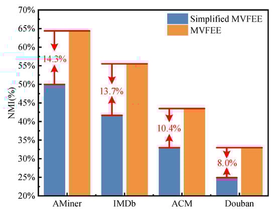
Figure 8.
Performance analysis of multi-view feature aggregation on edge clustering.
4.4. Link Prediction
The third experimental goal was to use link prediction as the task to evaluate the performance of the MVFEE model and multi-view feature aggregation strategy. We used ACC and AUC as evaluation metrics.
4.4.1. Performance Analysis of Our MVFEE Model
Similar to the above two tasks, this experiment used the same datasets and settings to verify the performance of the MVFEE on the link prediction task.
The link prediction accuracy (based on ACC (Figure 9a–c) and AUC (Figure 9a′–c′) for six algorithms is presented in Figure 9. The results indicate that these algorithms performed well and achieved an average performance of 0.51 and 0.60 for ACC and AUC, respectively. Further analysis of the results shows several important insights. (1) Comparing the six models, the MVFEE model outperformed all other models on all three networks, with Edge2vec performing second best. In contrast, HIN2vec had the poorest performance, while HAN, AspEm, and HEER had varying degrees of performance. (2) Considering different embedding methods, the edge embedding models (MVFEE, Edge2vec, AspEM, and HEER) achieved superior performance than the node embedding models (HAN and HIN2vec), and MVFEE outperformed all other edge embedding models on all networks. For example, MVFEE had an ACC score of 0.6818 on the AMiner network, compared to 0.6435 for HIN2vec. Similarly, Edge2vec had an AUC score of 0.5186 on the Douban network, while HIN2vec only achieved 0.4859. (3) Focusing on the edge embedding models, MVFEE outperformed other models on all three networks, and Edge2vec had better performance than AspEm and HEER. For example, on the ACM network, ACC scores for MVFEE, Edge2vec, AspEm, and HEER were 0.5117, 0.5013, 0.4874, and 0.4849, respectively. (4) Considering the depth of the edge embedding models, our shallow MVFEE model achieved better performance compared to the deeper CensNet model on most of the networks examined. For example, on the ACM network, MVFEE attained an AUC score of 0.5865, while CensNet only reached a score of 0.5787. (5) Considering the network density, the link prediction accuracy of all six models was higher on sparser networks (AMiner and ACM) than on denser ones (Douban). For example, ACC and AUC of MVFEE were highest on the AMiner network, with values of 0.6818 and 0.7573, respectively, while the best the model could achieve on the Douban network was an ACC of 0.4156 and an AUC of 0.5238. These results illustrate the effectiveness of edge embedding methods for the link prediction task and the superior performance of MVFEE for link prediction on different networks.
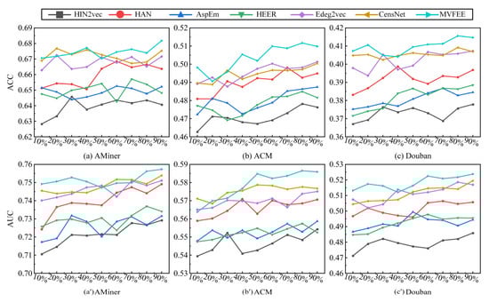
Figure 9.
Performance analysis of multiple algorithms on link prediction.
4.4.2. Performance Analysis of Multi-View Feature Aggregation
Similar to edge classification and edge clustering, this experiment used the same datasets and settings to verify the performance of the MVFEE model and the simplified MVFEE on the link prediction task, using ACC and AUC as evaluation metrics.
Figure 10 depicts the link prediction accuracy of both models on four networks, where ACC scores are presented in Figure 10a, and AUC scores are shown in Figure 10b. Based on the results, the following observations can be made. (1) Comparing the two models, the MVFEE model delivered higher scores in terms of both ACC and AUC scores on all four networks when compared to the simplified model. For example, on the AMiner network, the ACC and AUC scores of the MVFEE model were 0.6858 and 0.7573, while the simplified MVFEE model only achieved 0.5467 and 0.6115 for ACC and AUC scores, respectively. (2) Focusing on the density of the network, the improvement in the accuracy of the MVFEE model was less significant in denser networks. For example, the AUC of the MVFEE model only improved by 9.5% on the Douban network compared to the simplified MVFEE model, while it improved by 12.3% on the IMDb network. This can be attributed to the MVFEE model’s ability to aggregate learned features using the multi-view feature aggregation strategy.
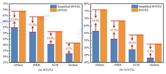
Figure 10.
Performance analysis of multi-view feature aggregation on link prediction.
4.5. Scalability
Scalability is a crucial factor for evaluating the performance of heterogeneous information network embedding models. With the rapid growth of network size, it is essential for a model to be able to handle large-scale networks in a reasonable amount of time. In this experiment, the intra-type feature learning process is parallelized using multi-threading techniques, and the ratio of parallelized threads to accelerated multipliers is recorded. The experimental results are shown in Figure 11.
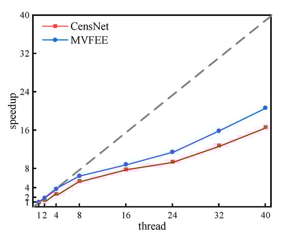
Figure 11.
The scalability performance of the MVFEE model.
The findings presented in Figure 11 illustrate the impact of the number of concurrent threads on the speedup multiplier. The plot shows that the MVFEE model achieves a significant speedup even with a lower number of threads. One of the notable observations is that MVFEE outperforms CensNet in terms of speedup when using multiple threads for concurrent execution. Specifically, when using 16 threads, MVFEE achieved a speedup of eight times compared to the baseline, while CensNet only achieved a speedup of seven times. However, the speedup for both models increases more slowly as the number of threads increases. For instance, when using 40 threads, the speedup for MVFEE is 20 times, whereas for CensNet, it is 16 times. These results highlight the ability of our proposed model to handle large-scale networks with millions of nodes and edges in a reasonable amount of time while maintaining or even surpassing the performance of existing models. The scalability and effectiveness of MVFEE demonstrated in this experiment suggest its potential for real-world applications on large-scale networks.
4.6. Parameter Sensitivity
The goal of this experiment is to assess the sensitivity of the hyperparameter Win. The window size Win is a hyper-parameter, where two vertexes within a window are each other’s neighbors. A larger Win can indicate that vertexes have higher-order neighbors. Moreover, both the intra-view features learning and the inter-view features learning use the same Win value. We choose link prediction as our experimental task and evaluate it using ACC as the metric, and select the AMiner, IMDb, ACM, and Douban datasets as appropriate testing datasets.
Figure 12 presents the link prediction accuracy of our model with different values of the Win parameter, with Figure 12a–d representing the ACC trend lines of the AMiner, IMDb, ACM, and Douban networks, respectively. From the figure, several findings can be derived. (1) Focusing on a single network, the ACC of the link prediction task increases initially and then decreases with the increase in the Win value. Specifically, the ACC increases before Win reaches two, then drops sharply after Win reaches two on the AMiner network, and the same trend is observed in the IMDb and ACM network. On the Douban network, three is the best value. This suggests that a Win value that is too small cannot capture all neighbor features of one edge in the network, while the Win value that is too large results in captured features that do not belong to edges. (2) Considering the density of the network, denser networks require a larger value of the Win parameter. The optimal value of Win on the Douban network, which is denser compared to AMiner, IMDb, and ACM, is three, whereas the best value on relatively sparse networks (AMiner, IMDb, and ACM) is two. This shows that denser networks typically contain more neighbor edges and, thus, relatively more feature information. (3) In summary, a shared best range of parameter Win for different networks is [,].
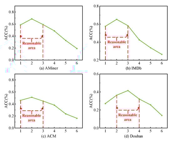
Figure 12.
Sensitivity analysis of the window size Win.
4.7. Visualization
To visually represent the performance of each model, we conducted a simple visualization experiment. First, we extracted a subset of 50 connected vertexes from the AMiner dataset, which contains millions of vertexes, to provide a clearer presentation. This extracted dataset consisted of four types of labeled vertexes, as well as unlabeled vertexes. Next, we extracted the edge embeddings of the entire AMiner network using partial baselines and MVFEE. We put these extracted edge embeddings into the edge classification task to predict the label of each vertex. By comparing the predicted labels with the true labels, we obtained the visualization results for the extracted 50 vertexes, which are depicted in Figure 13.
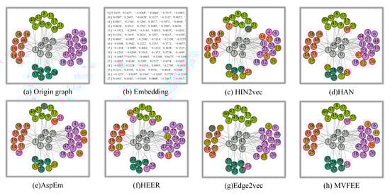
Figure 13.
Visualization of baselines and MVFEE on AMiner.
In Figure 13, different colors indicate different labels, and red numbers indicate incorrect classifications. The gray vertexes are unlabeled, and the rest of the colors are labeled vertexes. Figure 13a shows the visualization results of the extracted dataset based on the real labels. Figure 13b shows the edge embedding of AMiner extracted by MVFEE. Figure 13c–h shows the visualization results based on the predicted labels obtained by different algorithms. Comparing the visualization results in Figure 13, it is evident that MVFEE and Edge2vec outperformed the other models in the edge classification task. Specifically, in the light green region, MVFEE misclassified only one vertex, whereas Edge2vec achieved a perfect classification with no misclassified vertexes. On the other hand, AspEm and HEER both had three misclassified vertexes in the light green region. In the orange region, MVFEE achieved perfect classification without any misclassified vertexes, while HIN2vec misclassified three vertexes. In the purple region, Edge2vec misclassified only two vertexes, while HAN misclassified three vertexes.
5. Conclusions
In this paper, we propose a multi-view learning-based fast edge embedding model for HINs called MVFEE. The MVFEE model has the ability to quickly and accurately capture the embedding vectors of the edges of HINs. (1) To better learn coupled and diverse features, the edge graph of the original network is first divided into multiple views. As a result, the global features of each edge are divided into intra-view local features and inter-view local features, and each local feature is simpler, purer, and easier to learn. (2) To speed up embedding learning, a multi-view learning strategy is used to generate the embedding vectors of edges in a divide-and-conquer manner, where the learning process for each view can be performed in parallel. (3) To further speed it up, the shallow network is used in the intra-view feature learning, and cross-view feature learning to replace the deep network to capture the edge features more quickly. Extensive experimental results on multiple networks and multiple tasks demonstrate the good performance of our model. In our forthcoming research, we intend to delve deeper into the exploration of several promising topics in the field. Specifically, we will focus on advancing the methods related to the joint embedding of nodes and edges within heterogeneous information networks, as well as the methods of attribute network embedding.
Author Contributions
Conceptualization, C.L., X.D., T.H. and L.C.; Writing—Original draft, C.L.; Formal analysis, C.L.; Supervision, C.L. and L.C.; Validation, X.D., T.H., G.D. and Y.H.; Writing—Reviewing and Editing, X.D. and Y.H.; Investigation, X.D. and T.H.; Visualization, T.H., L.C. and Y.H.; Resources, L.C.; Methodology, G.D. and Y.H.; Data curation, G.D. All authors have read and agreed to the published version of the manuscript.
Funding
This research was funded by the National Key Research and Development Program (No. 2019YFE0105300); the National Natural Science Foundation of China (No. 62103143); the Hunan Province Key Research and Development Program (No. 2022WK2006); the Special Project for the Construction of Innovative Provinces in Hunan (No. 2020TP2018 and 2019GK4030); the Young Backbone Teacher of Hunan Province (No. 2022101); Hunan Provincial Natural Science Foundation of China (No. 2021JJ40214) and the Scientific Research Fund of Hunan Provincial Education Department (No. 22B0471 and 22C0829).
Data Availability Statement
The datasets could be downloaded at http://arnetminer.org/aminernetwork (10 March 2023), https://datasets.imdbws.com/ (10 March 2023), https:/www.aminer.org/citation (10 March 2023), https://www.dropbox.com/s/u2ejjezjk08lz1o/Douban.tar.gz?dl=0 (10 March 2023).
Conflicts of Interest
The authors declare no conflict of interest.
References
- Xiang, L.; Yu, Y.; Zhu, J. Moment-based analysis of pinning synchronization in complex networks. Asian J. Control 2022, 24, 669–685. [Google Scholar] [CrossRef]
- Chen, L.; Wang, L.; Zeng, C.; Liu, H.; Chen, J. DHGEEP: A Dynamic Heterogeneous Graph-Embedding Method for Evolutionary Prediction. Mathematics 2022, 10, 4193. [Google Scholar] [CrossRef]
- Zhang, C.; Li, K.; Wang, S.; Zhou, B.; Wang, L.; Sun, F. Learning Heterogeneous Graph Embedding with Metapath-Based Aggregation for Link Prediction. Mathematics 2023, 11, 578. [Google Scholar] [CrossRef]
- Chen, L.; Li, Y.; Deng, X.; Liu, Z.; Lv, M.; He, T. Semantic-aware network embedding via optimized random walk and paragaraph2vec. J. Comput. Sci. 2022, 63, 101825. [Google Scholar] [CrossRef]
- Huang, C.; Fang, Y.; Lin, X.; Cao, X.; Zhang, W. ABLE: Meta-Path Prediction in Heterogeneous Information Networks. ACM Trans. Knowl. Discov. Data 2022, 16, 1–21. [Google Scholar] [CrossRef]
- Huang, C.; Fang, Y.; Lin, X.; Cao, X.; Zhang, W.; Orlowska, M. Estimating Node Importance Values in Heterogeneous Information Networks. In Proceedings of the 38th International Conference on Data Engineering (ICDE), Kuala Lumpur, Malaysia, 9–12 May 2022; pp. 846–858. [Google Scholar]
- Luo, L.; Fang, Y.; Cao, X.; Zhang, X.; Zhang, W. Detecting Communities from Heterogeneous Graphs: A Context Path-based Graph Neural Network Model. In Proceedings of the 30th ACM International Conference on Information & Knowledge Management, Virtual Event, 1–5 November 2021; pp. 1170–1180. [Google Scholar]
- Wang, X.; Bo, D.; Shi, C.; Fan, S.; Ye, Y.; Philip, S.Y. A survey on heterogeneous graph embedding: Methods, techniques, applications and sources. IEEE Trans. Big Data 2022, 9, 415–436. [Google Scholar] [CrossRef]
- Chen, L.; Chen, F.; Liu, Z.; Lv, M.; He, T.; Zhang, S. Parallel gravitational clustering based on grid partitioning for large-scale data. Appl. Intell. 2022, 53, 2506–2526. [Google Scholar] [CrossRef]
- Lei, Y.; Chen, L.; Li, Y.; Xiao, R.; Liu, Z. Robust and fast representation learning for heterogeneous information networks. Front. Phys. 2023, 11, 357. [Google Scholar] [CrossRef]
- Shi, C.; Hu, B.; Zhao, W.X.; Philip, S.Y. Heterogeneous information network embedding for recommendation. IEEE Trans. Knowl. Data Eng. 2018, 31, 357–370. [Google Scholar] [CrossRef]
- Fu, T.; Lee, W.C.; Lei, Z. Hin2vec: Explore meta-paths in heterogeneous information networks for representation learning. In Proceedings of the 2017 ACM on Conference on Information and Knowledge Management, Singapore, 6–10 November 2017; pp. 1797–1806. [Google Scholar]
- Wang, X.; Ji, H.; Shi, C.; Wang, B.; Ye, Y.; Cui, P.; Yu, P.S. Heterogeneous graph attention network. In Proceedings of the World Wide Web Conference, San Francisco, CA, USA, 13–17 May 2019; pp. 2022–2032. [Google Scholar]
- Grover, A.; Leskovec, J. node2vec: Scalable feature learning for networks. In Proceedings of the 22nd ACM SIGKDD International Conference on Knowledge Discovery and Data Mining, San Francisco, CA, USA, 13–17 August 2016; pp. 855–864. [Google Scholar]
- Shi, Y.; Gui, H.; Zhu, Q.; Kaplan, L.; Han, J. Aspem: Embedding learning by aspects in heterogeneous information networks. In Proceedings of the 2018 SIAM International Conference on Data Mining. Society for Industrial and Applied Mathematics, San Diego, CA, USA, 3–5 May 2018; pp. 144–152. [Google Scholar]
- Shi, Y.; Zhu, Q.; Guo, F.; Zhang, C.; Han, J. Easing embedding learning by comprehensive transcription of heterogeneous information networks. In Proceedings of the 24th ACM SIGKDD International Conference on Knowledge Discovery & Data Mining, London, UK, 19–23 August 2018; pp. 2190–2199. [Google Scholar]
- Veličković, P.; Cucurull, G.; Casanova, A.; Romero, A.; Lio, P.; Bengio, Y. Graph attention networks. arXiv 2017, arXiv:1710.10903. [Google Scholar] [CrossRef]
- Kipf, T.N.; Welling, M. Semi-supervised classification with graph convolutional networks. arXiv 2016, arXiv:1609.02907. [Google Scholar]
- Goodfellow, I.; Pouget-Abadie, J.; Mirza, M.; Xu, B.; Warde-Farley, D.; Ozair, S.; Courville, A.; Bengio, Y. Generative adversarial networks. Commun. ACM 2020, 63, 139–144. [Google Scholar] [CrossRef]
- Chen, L.; Zheng, H.; Li, Y.; Liu, Z.; Zhao, L.; Tang, H. Enhanced density peak-based community detection algorithm. J. Intell. Inf. Syst. 2022, 59, 263–284. [Google Scholar] [CrossRef]
- Chen, L.; Guo, Q.; Liu, Z.; Zhang, S.; Zhang, H. Enhanced synchronization-inspired clustering for high-dimensional data. Complex Intell. Syst. 2021, 7, 203–223. [Google Scholar] [CrossRef]
- Hamilton, W.; Ying, Z.; Leskovec, J. Inductive representation learning on large graphs. arXiv 2017, arXiv:1706.02216. [Google Scholar]
- Wang, C.; Wang, C.; Wang, Z.; Ye, X.; Yu, P.S. Edge2vec: Edge-based social network embedding. ACM Trans. Knowl. Discov. Data (TKDD) 2020, 14, 1–24. [Google Scholar] [CrossRef]
- Chen, H.; Koga, H. Gl2vec: Graph embedding enriched by line graphs with edge features. In Proceedings of the Neural Information Processing: 26th International Conference, ICONIP 2019, Sydney, Australia, 12–15 December 2019; Proceedings, Part III 26. Springer International Publishing: Cham, Switzerland, 2019; pp. 3–14. [Google Scholar]
- Jiang, X.; Zhu, R.; Li, S.; Ji, P. Co-embedding of nodes and edges with graph neural networks. IEEE Trans. Pattern Anal. Mach. Intell. 2020, 45, 7075–7086. [Google Scholar] [CrossRef] [PubMed]
- Lozano, M.A.; Escolano, F.; Curado, M.; Hancock, E.R. Network embedding from the line graph: Random walkers and boosted classification. Pattern Recognit. Lett. 2021, 143, 36–42. [Google Scholar] [CrossRef]
- Tang, J.; Zhang, J.; Yao, L.; Li, J.; Zhang, L.; Su, Z. ArnetMiner: Extraction and Mining of Academic Social Networks. In Proceedings of the Fourteenth ACM SIGKDD International Conference on Knowledge Discovery and Data Mining (SIGKDD’2008), Las Vegas, NV, USA, 24–27 August 2008; pp. 990–998. [Google Scholar]
- Song, W.; Xiao, Z.; Wang, Y.; Charlin, L.; Zhang, M.; Tang, J. Session-based social recommendation via dynamic graph attention networks. In Proceedings of the Twelfth ACM International Conference on Web Search and Data Mining, Melbourne, Australia, 11–15 February 2019; pp. 555–563. [Google Scholar]
- Aggarwal, C.; He, G.; Zhao, P. Edge classification in networks. In Proceedings of the 2016 IEEE 32nd International Conference on Data Engineering (ICDE), Helsinki, Finland, 16–20 May 2016; pp. 1038–1049. [Google Scholar]
- Cai, B.; Wang, Y.; Zeng, L.; Hu, Y.; Li, H. Edge classification based on Convolutional Neural Networks for community detection in complex network. Phys. A Stat. Mech. Its Appl. 2020, 556, 124826. [Google Scholar] [CrossRef]
- Kim, P.; Kim, S. Detecting overlapping and hierarchical communities in complex network using interaction-based edge clustering. Phys. A Stat. Mech. Its Appl. 2015, 417, 46–56. [Google Scholar] [CrossRef]
- Zhang, X.K.; Tian, X.; Li, Y.N.; Song, C. Label propagation algorithm based on edge clustering coefficient for community detection in complex networks. Int. J. Mod. Phys. B 2014, 28, 1450216. [Google Scholar] [CrossRef]
- Hu, B.; Fang, Y.; Shi, C. Adversarial learning on heterogeneous information networks. In Proceedings of the 25th ACM SIGKDD International Conference on Knowledge Discovery & Data Mining, Anchorage, AK, USA, 4–8 August 2019; pp. 120–129. [Google Scholar]
- Zhang, C.; Swami, A.; Chawla, N.V. Shne: Representation learning for semantic-associated heterogeneous networks. In Proceedings of the Twelfth ACM International Conference on Web Search and Data Mining, Melbourne, Australia, 11–15 February 2019; pp. 690–698. [Google Scholar]
Disclaimer/Publisher’s Note: The statements, opinions and data contained in all publications are solely those of the individual author(s) and contributor(s) and not of MDPI and/or the editor(s). MDPI and/or the editor(s) disclaim responsibility for any injury to people or property resulting from any ideas, methods, instructions or products referred to in the content. |
© 2023 by the authors. Licensee MDPI, Basel, Switzerland. This article is an open access article distributed under the terms and conditions of the Creative Commons Attribution (CC BY) license (https://creativecommons.org/licenses/by/4.0/).