Geary’s c and Spectral Graph Theory: A Complement

Abstract

Spatial autocorrelation, which describes the similarity between signals on adjacent vertices, is central to spatial science, and Geary’s c is one of the most-prominent numerical measures of it. Using concepts from spectral graph theory, this paper documents new theoretical results on the measure. MATLAB/GNU Octave user-defined functions are also provided.

1. Introduction

Using concepts from spectral graph theory, in this paper, we document new theoretical results on Geary’s c, which is one of the most-prominent numerical measures of spatial autocorrelation. (Moran’s I is another prominent numerical measure. For the measure, see, e.g., [1,2].) Here, spatial autocorrelation describes the similarity between signals on adjacent vertices and is central to spatial science ([3]). Therefore, the results about the measure contribute to the development of spatial science.

More specifically, we provide a new representation of Geary’s c. It is an expansion of it into a linear combination of variables with different degrees of spatial autocorrelation. By using the distribution of the coefficients, we can characterize spatial data. It is somewhat similar to Fourier series. Subsequently, we develop a way to compute the graph Laplacian eigenvectors needed for the graph Fourier transform. MATLAB/GNU Octave user-defined functions are also provided.

This paper can be considered complementary to [4]. As in this paper, using concepts from spectral graph theory, [4] provided three types of representations for it: (a) graph Laplacian representation, (b) graph Fourier transform representation, and (c) Pearson’s correlation coefficient representation. Our new representation can be regarded as an addition to them. Moreover, the way to compute the graph Laplacian eigenvectors is useful not only for this paper, but also for [4].

We make two remarks on Geary’s c. First, Geary’s c was developed by [5] and modified by [6,7,8,9]) into what it is today. It is a spatial generalization of the von Neumann ratio ([10]). Second, unlike Pearson’s correlation coefficient, there exists the following:

$$\begin{array}{c}\hfill \left\{\begin{array}{cc}\mathrm{Positive}\mathrm{spatial}\mathrm{autocorrelation}\hfill & \mathrm{if}c<1;\hfill \\ \mathrm{No}\mathrm{spatial}\mathrm{autocorrelation}\hfill & \mathrm{if}c=1;\hfill \\ \mathrm{Negative}\mathrm{spatial}\mathrm{autocorrelation}\hfill & \mathrm{if}c>1.\hfill \end{array}\right.\end{array}$$

See, e.g., [11] (Equation (6)).

This paper is organized as follows. In Section 2, we provide some preliminaries for the following two sections. In Section 3, we present a new representation of Geary’s c. In Section 4, we develop a way to compute the graph Laplacian eigenvectors needed for the graph Fourier transform. Section 5 concludes. In Appendix A, we provide MATLAB/GNU Octave user-defined functions.

Some Notations

Let $\mathit{y}={[y_1,\dots ,y_n]}^{\top }$, ${\mathit{I}}_n$ be the identity matrix of order n and $\mathit{\iota }$ be the n-dimensional column vector of ones, i.e., $\mathit{\iota }={[1,\dots ,1]}^{\top }$. For an $n\times m$ full column rank matrix $\mathit{A}$, denote the column space of $\mathit{A}$ and its orthogonal complement by $\mathbb{S}\left(\mathit{A}\right)$ and ${\mathbb{S}}^{\perp }\left(\mathit{A}\right)$, respectively. For square matrices ${\mathit{A}}_1,\dots ,{\mathit{A}}_p$, $\mathrm{diag}({\mathit{A}}_1,\dots ,{\mathit{A}}_p)$ denotes the block diagonal matrix, whose diagonals are ${\mathit{A}}_1,\dots ,{\mathit{A}}_p$.

2. Preliminaries

Let $y_i$ denote the realization of a variable on a spatial unit i for $i=1,\dots ,n$. Here, we exclude the case where $y_1=\cdots =y_n$, i.e., $\mathit{y}\notin \mathbb{S}\left(\mathit{\iota }\right)$. Accordingly, ${\sum }_{i=1}^n{(y_i-\overline{y})}^2>0$, where $\overline{y}=\frac{1}{n}{\sum }_{i=1}^n{y}_i$. In addition, let $w_{ij}$ be the nonnegative spatial weight between the spatial units i and j. Here, we suppose that $w_{ii}=0$ and $w_{ji}=w_{ij}$ for $i,j=1,\dots ,n$. Accordingly, the spatial weights matrix $\mathit{W}=\left[w_{ij}\right]$ is an $n\times n$ symmetric hollow matrix. In addition, let $\mathrm{\Omega }={\sum }_{i=1}^n{\sum }_{j=1}^n{w}_{ij}$, which is assumed positive.

Geary’s c for $\mathit{y}$, denoted by $c\left(\mathit{y}\right)$, is defined by

$$\begin{array}{c}\hfill c\left(\mathit{y}\right)=\frac{n-1}{2\mathrm{\Omega }}\frac{{\sum }_{i=1}^n{\sum }_{j=1}^n{w}_{ij}{(y_i-y_j)}^2}{{\sum }_{i=1}^n{(y_i-\overline{y})}^2}.\end{array}$$

(1)

Let $\mathit{D}=\mathrm{diag}(d_1,\dots ,d_n)$, where $d_i={\sum }_{j=1}^n{w}_{ij}$ for $i=1,\dots ,n$. Then, the graph Laplacian in spectral graph theory (see, e.g., [12,13,14]) is defined as

$$\begin{array}{c}\hfill \mathit{L}=\mathit{D}-\mathit{W}.\end{array}$$

(2)

Accordingly, as shown in, e.g., [4,14], $\mathit{L}$ is a nonnegative definite matrix such that $\mathit{L}\mathit{\iota }=\mathbf{0}$.

Ref. [4] (Proposition 3.1) showed that $c\left(\mathit{y}\right)$ can be represented using $\mathit{L}$ as

$$\begin{array}{c}\hfill c\left(\mathit{y}\right)=\frac{n-1}{\mathrm{\Omega }}\frac{{\mathit{y}}^{\top }\mathit{L}\mathit{y}}{{\mathit{y}}^{\top }{\mathit{Q}}_{\iota }\mathit{y}},\end{array}$$

(3)

where ${\mathit{Q}}_{\iota }={\mathit{I}}_n-\mathit{\iota }{\left({\mathit{\iota }}^{\top }\mathit{\iota }\right)}^{-1}{\mathit{\iota }}^{\top }$, which is a symmetric idempotent matrix, i.e., ${\mathit{Q}}_{\iota }^{\top }={\mathit{Q}}_{\iota }$ and ${\mathit{Q}}_{\iota }^2={\mathit{Q}}_{\iota }$.

Given that $\mathit{L}$ is a real symmetric matrix, it can be spectrally decomposed as

$$\begin{array}{c}\hfill \mathit{L}=\mathit{U}\mathbf{\Lambda }{\mathit{U}}^{\top },\end{array}$$

(4)

where $\mathbf{\Lambda }=\mathrm{diag}({\lambda }_1,\dots ,{\lambda }_n)$ and $\mathit{U}=[{\mathit{u}}_1,\dots ,{\mathit{u}}_n]$ is an orthogonal matrix. Here, $({\lambda }_k,{\mathit{u}}_k)$ denotes an eigenpair of $\mathit{L}$ for $k=1,\dots ,n$, and the eigenvalues, ${\lambda }_1,\dots ,{\lambda }_n$, are in ascending order. Given that $\mathit{L}$ is a nonnegative definite matrix and $\mathit{L}\mathit{\iota }=\mathbf{0}$, we can suppose that $({\lambda }_1,{\mathit{u}}_1)=\left(0,\frac{1}{\sqrt{n}}\mathit{\iota }\right)$. Let m denote the number of connected components. Then, it is known that $0={\lambda }_1=\cdots ={\lambda }_m<{\lambda }_{m+1}\le \cdots \le {\lambda }_n$. See, e.g., [14]. Let ${\mathbf{\Lambda }}_2=\mathrm{diag}({\lambda }_2,\dots ,{\lambda }_n)$ and ${\mathit{U}}_2=[{\mathit{u}}_2,\dots ,{\mathit{u}}_n]$. We show how to obtain ${\mathit{U}}_2$, as well as ${\mathbf{\Lambda }}_2$ from $\mathit{L}$ in Section 4.

In spectral graph theory, the linear transformation given by ${\mathit{U}}^{\top }\mathit{y}$ is referred to as the graph Fourier transform of $\mathit{y}$ ([15]). In addition, ${\lambda }_k$ and ${\mathit{u}}_k$ for $k=1,\dots ,n$ are referred to as graph Laplacian eigenvalues and graph Laplacian eigenvectors, respectively. Let ${[{\alpha }_1,\dots ,{\alpha }_n]}^{\top }={\mathit{U}}^{\top }\mathit{y}$.

Given that ${\mathit{u}}_1\in \mathbb{S}\left(\mathit{\iota }\right)$, ${\mathit{u}}_k\in {\mathbb{S}}^{\perp }\left(\mathit{\iota }\right)$ for $k=2,\dots ,n$, and ${\mathit{Q}}_{\iota }$ is an orthogonal projection matrix onto ${\mathbb{S}}^{\perp }\left(\mathit{\iota }\right)$, it follows that ${\mathit{Q}}_{\iota }\mathit{U}=[\mathbf{0},{\mathit{u}}_2,\dots ,{\mathit{u}}_n]$, which yields

$$\begin{array}{c}\hfill {\mathit{y}}^{\top }{\mathit{Q}}_{\iota }\mathit{U}=[0,{\alpha }_2,\dots ,{\alpha }_n].\end{array}$$

(5)

In addition, given that $\mathit{L}$ is symmetric and $\mathit{L}\mathit{\iota }=\mathbf{0}$, it follows that

$$\begin{array}{c}\hfill \mathit{L}={\mathit{Q}}_{\iota }\mathit{L}{\mathit{Q}}_{\iota }.\end{array}$$

(6)

Moreover, $\mathit{U}$ is an orthogonal matrix. By combining these results, $c\left(\mathit{y}\right)$ can be represented as

$$\begin{array}{c}\hfill c\left(\mathit{y}\right)=\frac{n-1}{\mathrm{\Omega }}\frac{{\mathit{y}}^{\top }{\mathit{Q}}_{\iota }\mathit{U}\mathbf{\Lambda }{\mathit{U}}^{\top }{\mathit{Q}}_{\iota }\mathit{y}}{{\mathit{y}}^{\top }{\mathit{Q}}_{\iota }\mathit{U}{\mathit{U}}^{\top }{\mathit{Q}}_{\iota }\mathit{y}}=\frac{n-1}{\mathrm{\Omega }}\frac{{\sum }_{k=2}^n{\lambda }_k{\alpha }_k^2}{{\sum }_{j=2}^n{\alpha }_j^2}.\end{array}$$

(7)

Here, given that $\mathit{y}\notin \mathbb{S}\left(\mathit{\iota }\right)$, it follows that ${\sum }_{j=2}^n{\alpha }_j^2={\mathit{y}}^{\top }{\mathit{Q}}_{\iota }\mathit{y}>0$. Finally, we note that (7) is a part of [4] (Proposition 3.3).

3. A New Representation of Geary’s $\mathit{c}$

Given that ${\mathit{u}}_k\notin \mathbb{S}\left(\mathit{\iota }\right)$ for $k=2,\dots ,n$, we can consider

$$\begin{array}{c}\hfill c\left({\mathit{u}}_k\right)=\frac{n-1}{\mathrm{\Omega }}\frac{{\mathit{u}}_k^{\top }\mathit{L}{\mathit{u}}_k}{{\mathit{u}}_k^{\top }{\mathit{Q}}_{\iota }{\mathit{u}}_k},k=2,\dots ,n,\end{array}$$

(8)

which can be regarded as Geary’s c when $\mathit{y}={\mathit{u}}_k$. We note that, given ${\mathit{u}}_1\in \mathbb{S}\left(\mathit{\iota }\right)$, Geary’s c when $\mathit{y}={\mathit{u}}_1$ is excluded. (Actually, it cannot be defined. This is because ${\mathit{u}}_1^{\top }{\mathit{Q}}_{\iota }{\mathit{u}}_1=0$.)

For $k=2,\dots ,n$, it follows that ${\mathit{u}}_k^{\top }\mathit{L}{\mathit{u}}_k={\mathit{u}}_k^{\top }\mathit{U}\mathbf{\Lambda }{\mathit{U}}^{\top }{\mathit{u}}_k={\mathit{e}}_k^{\top }\mathbf{\Lambda }{\mathit{e}}_k={\lambda }_k$ and ${\mathit{u}}_k^{\top }{\mathit{Q}}_{\iota }{\mathit{u}}_k={\parallel {\mathit{u}}_k\parallel }^2=1$, where ${\mathit{e}}_k$ is the k-th column of ${\mathit{I}}_n$. Thus, $c\left({\mathit{u}}_k\right)$ in (8) can be represented as

$$\begin{array}{c}\hfill c\left({\mathit{u}}_k\right)=\frac{n-1}{\mathrm{\Omega }}{\lambda }_k,k=2,\dots ,n.\end{array}$$

(9)

Then, from the inequalities, $0\le {\lambda }_2\le \cdots \le {\lambda }_n$, it follows that

$$\begin{array}{c}\hfill 0\le c\left({\mathit{u}}_2\right)\le \cdots \le c\left({\mathit{u}}_n\right).\end{array}$$

(10)

Moreover, given that ${\sum }_{k=2}^n{\lambda }_k={\sum }_{k=1}^n{\lambda }_k=\mathrm{tr}\left(\mathit{L}\right)=\mathrm{\Omega }$, it follows that

$$\begin{array}{c}\hfill \frac{1}{n-1}\sum _{k=2}^{n}c\left({\mathit{u}}_k\right)=\frac{1}{n-1}\sum _{k=2}^n\frac{n-1}{\mathrm{\Omega }}{\lambda }_k=1.\end{array}$$

(11)

By combining (7) and (9), we obtain

$$\begin{array}{cc}\hfill c\left(\mathit{y}\right)& =\frac{n-1}{\mathrm{\Omega }}\frac{{\sum }_{k=2}^n{\lambda }_k{\alpha }_k^2}{{\sum }_{j=2}^n{\alpha }_j^2}=\frac{{\sum }_{k=2}^n\left(\frac{n-1}{\mathrm{\Omega }}{\lambda }_k\right){\alpha }_k^2}{{\sum }_{j=2}^n{\alpha }_j^2}=\frac{{\sum }_{k=2}^{n}c\left({\mathit{u}}_k\right){\alpha }_k^2}{{\sum }_{j=2}^n{\alpha }_j^2}\hfill \\ \hfill & =\sum _{k=2}^n\left(\frac{{\alpha }_k^2}{{\sum }_{j=2}^n{\alpha }_k^2}\right)c\left({\mathit{u}}_k\right)=\sum _{k=2}^n{\psi }_{k}c\left({\mathit{u}}_k\right),\hfill \end{array}$$

(12)

where

$$\begin{array}{c}\hfill {\psi }_k=\frac{{\alpha }_k^2}{{\sum }_{j=2}^n{\alpha }_j^2},k=2,\dots ,n.\end{array}$$

(13)

Note that ${\psi }_k$ in (13) satisfy ${\psi }_k\ge 0$ and ${\sum }_{k=2}^n{\psi }_k=1$.

The next proposition summarizes the above-mentioned results.

Proposition 1.

(a) $c\left(\mathit{y}\right)$ in (1) can be represented as ${\sum }_{k=2}^n{\psi }_{k}c\left({\mathit{u}}_k\right)$, where ${\psi }_k=\frac{{\alpha }_k^2}{{\sum }_{j=2}^n{\alpha }_j^2}$ for $k=2,\dots ,n$. Here, ${\psi }_k$ for $k=2,\dots ,n$ are nonnegative and sum to unity. (b) $c\left({\mathit{u}}_k\right)$ for $k=2,\dots ,n$ satisfy the inequalities given by (10), and their simple average equals unity.

Remark 1.

Concerning Proposition 1, we make three remarks:

(i) 

Proposition 1(a) implies that Geary’s c can be represented as a weighted average of $c\left({\mathit{u}}_2\right),\dots ,c\left({\mathit{u}}_n\right)$. Concerning the weight, ${\psi }_k$, the larger $|{\alpha }_k|=|{\mathit{u}}_k^{\top }\mathit{y}|=|{\left({\mathit{u}}_k^{\top }{\mathit{u}}_k\right)}^{-1}{\mathit{u}}_k^{\top }\mathit{y}|$ is, the larger ${\psi }_k$ is. We note that ${\alpha }_k=\mathit{arg}{min}_{{\varphi }_k}\parallel \mathit{y}-{\varphi }_1{\mathit{u}}_1-\cdots -{\varphi }_n{\mathit{u}}_n{\parallel }^2=\mathit{arg}{min}_{{\varphi }_k}{\parallel \mathit{y}-{\varphi }_k{\mathit{u}}_k\parallel }^2$.

(ii) 

Proposition 1(b) implies that the graph Laplacian eigenvectors, ${\mathit{u}}_2,\dots ,{\mathit{u}}_n$, can be sorted in the spatial autocorrelation measured by Geary’s c. In other words, ${\mathit{u}}_k$ is more positively spatially autocorrelated than or equal to ${\mathit{u}}_{k+1}$ for $k=2,\dots ,n-1$. Accordingly, $\mathit{y}$ is positively (respectively negatively) spatially autocorrelated if $\left\{{\psi }_k\right\}$ is a monotonically decreasing (respectively increasing) sequence. $\mathit{y}$ can be characterized by the distribution of the coefficients, ${\psi }_2,\dots ,{\psi }_n$. It is somewhat similar to the Fourier series.

(iii) 

If $c\left({\mathit{u}}_2\right)=\cdots =c\left({\mathit{u}}_n\right)=\mu$, then $c\left(\mathit{y}\right)={\sum }_{k=2}^n{\psi }_{k}c\left({\mathit{u}}_k\right)=\mu {\sum }_{k=2}^n{\psi }_k=\mu$ regardless of $\mathit{y}$.

Let $\mathit{\eta }={\mathit{\eta }}_1+{\mathit{\eta }}_2$, where ${\mathit{\eta }}_1\in \mathbb{S}\left(\mathit{\iota }\right)$ and ${\mathit{\eta }}_2\in \mathbb{S}\left(\mathit{y}\right)\setminus \left\{\mathbf{0}\right\}$. Then, $c\left(\mathit{\eta }\right)$ equals $c\left(\mathit{y}\right)$. That is, for all ${\gamma }_1\in \mathbb{R}$ and ${\gamma }_2\in \mathbb{R}\setminus \left\{0\right\}$, it follows that

$$\begin{array}{c}\hfill c({\gamma }_1\mathit{\iota }+{\gamma }_2\mathit{y})=c\left(\mathit{y}\right).\end{array}$$

(14)

Given that ${\mathit{Q}}_{\iota }\mathit{y}=\mathit{y}-\overline{y}\mathit{\iota }$, $c\left({\mathit{Q}}_{\iota }\mathit{y}\right)=c\left(\mathit{y}\right)$ is an example of (14). From (14) and Proposition 1(a), we obtain $c({\gamma }_1\mathit{\iota }+{\gamma }_2\mathit{y})={\sum }_{k=2}^n{\psi }_{k}c\left({\mathit{u}}_k\right)$.

The next corollary summarizes the above result.

Corollary 1.

For all ${\gamma }_1\in \mathbb{R}$ and ${\gamma }_2\in \mathbb{R}\setminus \left\{0\right\}$, $c({\gamma }_1\mathit{\iota }+{\gamma }_2\mathit{y})$ equals ${\sum }_{k=2}^n{\psi }_{k}c\left({\mathit{u}}_k\right)$.

In addition, from Proposition 1, it immediately follows that

$$\begin{array}{c}\hfill c\left(\mathit{y}\right)=\sum _{k=2}^n{\psi }_{k}c\left({\mathit{u}}_k\right)\le \sum _{k=2}^n{\psi }_{k}c\left({\mathit{u}}_n\right)=c\left({\mathit{u}}_n\right)\sum _{k=2}^n{\psi }_k=c\left({\mathit{u}}_n\right).\end{array}$$

(15)

Likewise, $c\left({\mathit{u}}_2\right)\le c\left(\mathit{y}\right)$ follows.

The next corollary summarizes the above result.

Corollary 2.

$c\left(\mathit{y}\right)$ belongs to the closed interval given by $\left[c\left({\mathit{u}}_2\right),c\left({\mathit{u}}_n\right)\right]$.

Remark 2.

Concerning Corollary 2, we make two remarks:

(i) 

If $c\left({\mathit{u}}_2\right)=\cdots =c\left({\mathit{u}}_n\right)$, then the interval given by $\left[c\left({\mathit{u}}_2\right),c\left({\mathit{u}}_n\right)\right]$ reduces to a singleton. For example, if $\mathit{W}=\mathit{\iota }{\mathit{\iota }}^{\top }-{\mathit{I}}_n$, which is the binary adjacency matrix of the complete graph with n vertices, then $\mathit{L}=(n-1){\mathit{I}}_n-(\mathit{\iota }{\mathit{\iota }}^{\top }-{\mathit{I}}_n)=n{\mathit{Q}}_{\iota }$ and, accordingly, $c\left({\mathit{u}}_2\right)=\cdots =c\left({\mathit{u}}_n\right)=\frac{n-1}{n(n-1)}\times n=1$. Then, in this case, $c\left(\mathit{y}\right)={\sum }_{k=2}^n{\psi }_{k}c\left({\mathit{u}}_k\right)={\sum }_{k=2}^n{\psi }_k=1$ regardless of $\mathit{y}$.

(ii) 

Ref. [11] showed that $c\left(\mathit{y}\right)$ belongs to the closed interval given by $\left[\frac{n-1}{\mathrm{\Omega }}{\lambda }_2,\frac{n-1}{\mathrm{\Omega }}{\lambda }_n\right]$. Given (9), Corollary 2 is its equivalent.

4. A Way to Compute the Eigenvectors in (4)

In this section, we develop a way to compute ${\mathit{U}}_2=[{\mathit{u}}_2,\dots ,{\mathit{u}}_n]$, which also provides ${\mathbf{\Lambda }}_2=\mathrm{diag}({\lambda }_2,\dots ,{\lambda }_n)$. Here, we explain the reason why it is useful. When there is only one connected component, i.e., $m=1$, there is no problem. This is because $\mathit{L}$ has single 0 eigenvalue and the corresponding normalized eigenvector is $\frac{1}{\sqrt{n}}\mathit{\iota }$. However, when there is more than one connected component, i.e., $m\ge 2$, $\mathit{L}$ has multiple 0 eigenvalues, and then, $\frac{1}{\sqrt{n}}\mathit{\iota }$ is not necessarily one of the eigenvectors returned from a computer program. For example, when

$$\begin{array}{c}\hfill \mathit{W}=\left[\begin{array}{ccccc}0& 1& 0& 0& 0\\ 1& 0& 1& 0& 0\\ 0& 1& 0& 0& 0\\ 0& 0& 0& 0& 1\\ 0& 0& 0& 1& 0\end{array}\right],\end{array}$$

(16)

there are two connected components and, accordingly, $m=2$ (Figure 1). In this case, both $(0,{\mathit{u}}_1^{*})$ and $(0,{\mathit{u}}_2^{*})$, where ${\mathit{u}}_1^{*}=\frac{1}{\sqrt{3}}{[1,1,1,0,0]}^{\top }$ and ${\mathit{u}}_2^{*}=\frac{1}{\sqrt{2}}{[0,0,0,1,1]}^{\top }$, and $(0,{\mathit{u}}_1)$ and $(0,{\mathit{u}}_2)$, where ${\mathit{u}}_1=\frac{1}{\sqrt{5}}{[1,1,1,1,1]}^{\top }$ and ${\mathit{u}}_2={\left[\sqrt{\frac{2}{15}},\sqrt{\frac{2}{15}},\sqrt{\frac{2}{15}},-\sqrt{\frac{3}{10}},-\sqrt{\frac{3}{10}}\right]}^{\top }$, are eigenpairs of the corresponding graph Laplacian. The results below can handle such a situation.

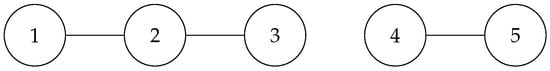
Figure 1. Undirected graph whose binary adjacency matrix is $\mathit{W}$ in (16).

Let $\{{\mathit{g}}_2,\dots ,{\mathit{g}}_n\}$ denote any orthonormal basis of ${\mathbb{S}}^{\perp }\left(\mathit{\iota }\right)$ and $\mathit{G}=[{\mathit{g}}_1,{\mathit{G}}_2]$, where ${\mathit{g}}_1=\frac{1}{\sqrt{n}}\mathit{\iota }$ and ${\mathit{G}}_2=[{\mathit{g}}_2,\dots ,{\mathit{g}}_n]$. Then, $\mathit{G}$ is an $n\times n$ orthogonal matrix. Accordingly, from (4) and (6), it follows that

$$\begin{array}{c}\hfill {\mathit{G}}^{\top }{\mathit{Q}}_{\iota }\mathit{L}{\mathit{Q}}_{\iota }\mathit{G}\mathit{V}=\mathit{V}\mathbf{\Lambda },\end{array}$$

(17)

where $\mathit{V}={\mathit{G}}^{\top }\mathit{U}$. Here, from ${\mathit{g}}_1^{\top }{\mathit{u}}_1=1$, ${\mathit{g}}_1^{\top }{\mathit{U}}_2=\mathbf{0}$, and ${\mathit{G}}_2^{\top }{\mathit{u}}_1=\mathbf{0}$, it follows that

$$\begin{array}{c}\hfill \mathit{V}=\mathrm{diag}(1,{\mathit{V}}_2),\end{array}$$

(18)

where ${\mathit{V}}_2={\mathit{G}}_2^{\top }{\mathit{U}}_2$, which is an $(n-1)\times (n-1)$ orthogonal matrix. This is because ${\mathit{V}}^{\top }\mathit{V}={\mathit{U}}^{\top }\mathit{G}{\mathit{G}}^{\top }\mathit{U}={\mathit{I}}_n$ and ${\mathit{V}}^{\top }\mathit{V}=\mathrm{diag}(1,{\mathit{V}}_2^{\top }{\mathit{V}}_2)$. In addition, given that ${\mathit{Q}}_{\iota }\mathit{G}=[\mathbf{0},{\mathit{G}}_2]$, it follows that

$$\begin{array}{c}\hfill {\mathit{G}}^{\top }{\mathit{Q}}_{\iota }\mathit{L}{\mathit{Q}}_{\iota }\mathit{G}=\mathrm{diag}(0,{\mathit{G}}_2^{\top }\mathit{L}{\mathit{G}}_2).\end{array}$$

(19)

By combining (18) and (19), (17) becomes $\mathrm{diag}(0,{\mathit{G}}_2^{\top }\mathit{L}{\mathit{G}}_2)·\mathrm{diag}(1,{\mathit{V}}_2)=\mathrm{diag}(1,{\mathit{V}}_2)·\mathrm{diag}({\lambda }_1,{\mathbf{\Lambda }}_2)$. Therefore, it follows that

$$\begin{array}{c}\hfill {\mathit{G}}_2^{\top }\mathit{L}{\mathit{G}}_2{\mathit{V}}_2={\mathit{V}}_2{\mathbf{\Lambda }}_2.\end{array}$$

(20)

Here, recall that ${\mathit{V}}_2$ is an orthogonal matrix. In addition, given that $\mathit{G}$ is an orthogonal matrix, premultiplying (18) by $\mathit{G}=[{\mathit{g}}_1,{\mathit{G}}_2]$ yields $\mathit{U}=[{\mathit{g}}_1,{\mathit{G}}_2]·\mathrm{diag}(0,{\mathit{V}}_2)=[{\mathit{g}}_1,{\mathit{G}}_2{\mathit{V}}_2]$. Therefore, it follows that

$$\begin{array}{c}\hfill {\mathit{U}}_2={\mathit{G}}_2{\mathit{V}}_2.\end{array}$$

(21)

The next proposition summarizes the above-mentioned results.

Proposition 2.

Denote the k-th column of ${\mathit{V}}_2$ by ${\mathit{v}}_{k+1}$ for $k=1,\dots ,n-1$, i.e., ${\mathit{V}}_2=[{\mathit{v}}_2,\dots ,{\mathit{v}}_n]$. Then, $({\lambda }_k,{\mathit{v}}_k)$ for $k=2,\dots ,n$ are the eigenpairs of ${\mathit{G}}_2^{\top }\mathit{L}{\mathit{G}}_2$. In addition, ${\mathit{U}}_2$ is obtainable from ${\mathit{V}}_2$ by (21).

Remark 3.

Concerning Proposition 2, we make two remarks:

(i) 

The following $n\times (n-1)$ matrix ${\mathit{F}}_2$ is an example of ${\mathit{G}}_2$:

$$\begin{array}{c}\hfill {\mathit{F}}_2=\left[\begin{array}{cccc}1& \cdots & \cdots & 1\\ -1& \ddots & & ⋮\\ 0& -2& \ddots & ⋮\\ ⋮& \ddots & \ddots & 1\\ 0& \cdots & 0& -(n-1)\end{array}\right]{\mathit{\Gamma }}^{-1},\end{array}$$

(22)

where $\mathit{\Gamma }=\mathrm{diag}(\sqrt{1·2},\dots ,\sqrt{(n-1)·n})$. (The use of ${\mathit{F}}_2$ is inspired by [16].) Here, $\mathit{F}=[{\mathit{f}}_1,{\mathit{F}}_2]$, where ${\mathit{f}}_1=\frac{1}{\sqrt{n}}\mathit{\iota }$, is a Helmert orthogonal matrix ([17]). Instead of ${\mathit{F}}_2$, we may use ${\mathit{H}}_2={\mathit{\Delta }}^{\top }{\left(\mathit{\Delta }{\mathit{\Delta }}^{\top }\right)}^{-\frac{1}{2}}$, where Δ is the $(n-1)\times n$ matrix such that $\mathit{\Delta }\mathit{\zeta }={[{\zeta }_2-{\zeta }_1,\dots ,{\zeta }_n-{\zeta }_{n-1}]}^{\top }$ for an n-dimensional vector $\mathit{\zeta }={[{\zeta }_1,\dots ,{\zeta }_n]}^{\top }$. This is because ${\mathit{H}}_2$ satisfies that ${\mathit{H}}_2^{\top }\mathit{\iota }={\left(\mathit{\Delta }{\mathit{\Delta }}^{\top }\right)}^{-\frac{1}{2}}\mathit{\Delta }\mathit{\iota }=\mathbf{0}$ and ${\mathit{H}}_2^{\top }{\mathit{H}}_2={\left(\mathit{\Delta }{\mathit{\Delta }}^{\top }\right)}^{-\frac{1}{2}}\mathit{\Delta }{\mathit{\Delta }}^{\top }{\left(\mathit{\Delta }{\mathit{\Delta }}^{\top }\right)}^{-\frac{1}{2}}={\mathit{I}}_{n-1}$. Here, $\mathit{\Delta }{\mathit{\Delta }}^{\top }$ is a positive definite matrix.

(ii) 

MATLAB/GNU Octave user-defined functions required for the calculation of ${\mathbf{\Lambda }}_2$, ${\mathit{U}}_2$, and the bounds of Geary’s c are provided in Appendix A.

5. Concluding Remarks

In this paper, we showed new theoretical results on Geary’s c, which included (i) a new representation of Geary’s c and (ii) a way to compute the graph Laplacian eigenvectors. The obtained results are summarized in Propositions 1 and 2 and Corollaries 1 and 2. The required MATLAB/GNU Octave user-defined functions are also provided. Finally, as stated, this paper can be considered complementary to [4].

References

- Dray, S. A new perspective about Moran’s coefficient: Spatial autocorrelation as a linear regression problem. Geogr. Anal. 2011, 43, 127–141. [Google Scholar]
- Yamada, H. A unified perspective on some autocorrelation measures in different fields: A note. Open Math. 2023, 21, 20220574. [Google Scholar] [CrossRef]
- Getis, A. A history of the concept of spatial autocorrelation: A geographer’s perspective. Geogr. Anal. 2008, 40, 297–309. [Google Scholar] [CrossRef]
- Yamada, H. Geary’s c and spectral graph theory. Mathematics 2021, 9, 2465. [Google Scholar] [CrossRef]
- Geary, R.C. The contiguity ratio and statistical mapping. Inc. Stat. 1954, 5, 115–127+129–146. [Google Scholar] [CrossRef]
- Cliff, A.D.; Ord, J.K. The problem of spatial autocorrelation. In Studies in Regional Science; Scott, A.J., Ed.; Pion: London, UK, 1969; pp. 25–55. [Google Scholar]
- Cliff, A.D.; Ord, J.K. Spatial autocorrelation: A review of existing and new measures with applications. Econ. Geogr. 1970, 46, 269–292. [Google Scholar] [CrossRef]
- Cliff, A.D.; Ord, J.K. Spatial Autocorrelation; Pion: London, UK, 1973. [Google Scholar]
- Cliff, A.D.; Ord, J.K. Spatial Processes: Models and Applications; Pion: London, UK, 1981. [Google Scholar]
- Von Neumann, J. Distribution of the ratio of the mean square successive difference to the variance. Ann. Math. Stat. 1941, 12, 367–395. [Google Scholar] [CrossRef]
- De Jong, P.; Sprenger, C.; van Veen, F. On extreme values of Moran’s I and Geary’s c. Geogr. Anal. 1984, 16, 17–24. [Google Scholar] [CrossRef]
- Bapat, R.B. Graphs and Matrices, 2nd ed.; Springer: London, UK, 2014. [Google Scholar]
- Estrada, E.; Knight, P. A First Course in Network Theory; Oxford University Press: Oxford, UK, 2015. [Google Scholar]
- Gallier, J. Spectral theory of unsigned and signed graphs. Applications to graph clustering: A survey. arXiv 2016, arXiv:1601.04692. [Google Scholar]
- Shuman, D.I.; Narang, S.K.; Frossard, P.; Ortega, A.; Vandergheynst, P. The emerging field of signal processing on graphs: Extending high-dimensional data analysis to networks and other irregular domains. IEEE Signal Process. Mag. 2013, 30, 83–98. [Google Scholar] [CrossRef]
- Maruyama, Y. An alternative to Moran’s I for spatial autocorrelation. arXiv 2015, arXiv:1501.06260v1. [Google Scholar]
- Lancaster, H.O. The Helmert Matrices. Am. Math. Mon. 1965, 72, 4–12. [Google Scholar] [CrossRef]
Disclaimer/Publisher’s Note: The statements, opinions and data contained in all publications are solely those of the individual author(s) and contributor(s) and not of MDPI and/or the editor(s). MDPI and/or the editor(s) disclaim responsibility for any injury to people or property resulting from any ideas, methods, instructions or products referred to in the content. |
© 2023 by the author. Licensee MDPI, Basel, Switzerland. This article is an open access article distributed under the terms and conditions of the Creative Commons Attribution (CC BY) license (https://creativecommons.org/licenses/by/4.0/).