Abstract
Ensuring the stability of surrounding rock is crucial for the safety of underground engineering projects. In this study, an improved fuzzy comprehensive evaluation method is proposed to accurately predict the stability of surrounding rock. Five key factors, namely, rock quality designation, uniaxial compressive strength, integrality coefficient of the rock mass, strength coefficient of the structural surface, and groundwater seepage, are selected as evaluation indicators, and a five-grade evaluation system is established. An improved analytic hierarchy process (IAHP) is proposed to enhance the accuracy of the evaluation. Using interval numbers rather than real numbers in constructing an interval judgment matrix can better account for the subjective fuzziness and uncertainty of expert judgment. Subjective and objective weights are obtained through IAHP and coefficient of variation, and the comprehensive weight is calculated on the basis of game theory principles. In addition, trapezoidal and triangular membership functions are employed to determine the membership degree, and an improved fuzzy comprehensive evaluation model is constructed. The model is then used to determine the stability of the surrounding rock based on the improved criterion. It is applied to six samples from an actual underground project in China to validate its effectiveness. Results show that the proposed model accurately and effectively predicts the stability of surrounding rock, which aligns with the findings from field investigations. The proposed method provides a valuable reference for evaluating surrounding rock stability and controlling construction risks.
Keywords:
surrounding rock stability; IAHP; fuzzy comprehensive evaluation; coefficient of variation MSC:
91A86
1. Introduction
The accelerated exploitation of underground resources has led to increased construction of underground engineering projects. The 21st century has been dubbed the “century of underground space” as more people live or work in such environments. Therefore, ensuring the safe construction of underground engineering is of paramount importance [1]. During the nonlinear excavation process of underground engineering, the stress field of the rock undergoes disturbance and redistribution [2]. These factors can lead to geological hazards, including rock burst, collapse, and water inrush. Determining the stability of the surrounding rock is a critical issue for construction safety [3]. It directly affects the economy, safety, and construction schedule of underground projects. Therefore, accurately assessing surrounding rock stability is vital for underground engineering.
The analysis of surrounding rock stability finds widespread application in water conservancy and hydropower engineering, mining engineering, and traffic engineering [4]. Numerous scholars have developed different evaluation methods based on various theories, which can be classified into analytical, numerical, and machine-learning approaches. Analytical methods include the Protodyakonov coefficient (f), rock quality designation (RQD), Q, and rock mass rating (RMR) method [5]. The Protodyakonov coefficient is simple but may introduce errors due to changes in stress states resulting from laboratory measurements [6]. RQD, proposed by Deere [7], offers a convenient indicator of rock quality. Beniawski developed the RMR system based on six parameters [8]. Barton proposed the Q system that evaluates rock mass quality using six different parameters [9]. However, these methods involve numerous parameters, some of which are difficult to determine accurately, leading to uncertainties regarding the mechanical properties of rock masses.
Other analytical methods include the Technique for Order Preference by Similarity to an Ideal Solution (TOPSIS) [10], the ideal point method [11], the matter-element method [12], and the cloud model approach [13]. Each of these methods has made remarkable contributions to the field. TOPSIS and the ideal point method calculate the closeness degree to obtain the results and address the quantification of indicator effects, which is a challenge for other methods. However, their results may fall between two grades. The matter-element method can ignore important constraints, leading to discrepancies between evaluation results and actual results. Cloud models construct a cloud generator to address the conversion of qualitative and quantitative data and consider the interaction of indicators. However, constructing cloud models is complex and challenging. Moreover, the evaluation index varies for different geotechnical projects [14].
Numerical methods include analytical fractal methods and numerical boundary element methods [15,16,17]. These approaches treat rock as porous media and examine its stability through the characterization of its complex structure. However, building fractal or numerical models is complex and time-consuming.
Many machine learning techniques, such as backpropagation (BP), Bayes, support vector machine (SVM), and random forest (RF), have been applied in the field of surrounding rock stability analysis [18,19]. Artificial intelligence algorithms possess strong nonlinear mapping capabilities and are widely used in engineering applications due to their effectiveness in regression prediction. Heuristic optimization algorithms, such as particle swarm optimization, genetic algorithms, gray wolf optimization, and Harris hawks optimizer methods, have been employed to enhance these techniques [20]. Machine learning methods utilize characteristic parameters of the rock mass as input to predict its stability by establishing a complex mapping relationship. This method improves the efficiency of stability prediction, reduces subjective judgment, and addresses parameter uncertainties associated with traditional methods. However, machine learning methods have certain drawbacks. They can be slow to converge, require long training cycles, and are susceptible to local optima. Moreover, these methods require a large number of practical engineering samples for training, and their accuracy is influenced by the data dimension and the volume of data. In addition, machine learning methods are often regarded as black boxes, leading to uncertainty in the output results.
In practical underground engineering, determining the stability of surrounding rock quickly and accurately within limited measured samples and time presents challenges. This study proposes an improved fuzzy comprehensive evaluation method (IFCEM) for determining surrounding rock stability. The method uses the improved analytic hierarchy process (IAHP) and coefficient of variation (CV) to determine the subjective weights (SW) and objective weights (OW) of evaluation indicators. Additionally, game theory is employed to determine the comprehensive weights (CW) of these indicators. Based on fuzzy theory, the proposed method establishes a mathematical model, determines membership functions, improves the traditional judgment criterion, and uses the confidence criterion to assess the stability of surrounding rock. The effectiveness of the method is validated through an underground project in China. The model enables rapid and objective determination of rock mass stability, aligning with the actual situation.
The structure of this article is as follows. Section 1 presents the research background. Section 2 introduces the methods employed. Section 3 determines the evaluation system for surrounding rock stability. Section 4 establishes the fuzzy comprehensive model and presents an engineering case study. Section 5 discusses the results. Section 6 provides the conclusion.
2. Methods
2.1. Improved Analytic Hierarchy Process
The AHP method proposed by Saaty is a commonly used approach to determine SW [21,22]. It is simple, practical, and widely used. In this method, the weights are calculated on the basis of a judgment matrix, and a consistency test is conducted [23].
In the traditional AHP, determining the scale of pairwise comparisons is crucial. During the process of comparison, experts may have limitations in their knowledge, leading to judgments that involve uncertainty. To address this issue, this study proposes an IAHP method that considers the importance of interval numbers in pairwise comparisons. This approach better aligns with the thinking of experts, resulting in weight outcomes that meet the requirements. The steps involved in the IAHP are as follows:
- (1)
- Construction of judgment matrix
Let the interval number be defined as , and multiple interval numbers are used to form a judgment matrix A. Experts are invited to provide the upper and lower limits of the interval numbers and and for pairwise comparisons between the two indexes. The values for the interval numbers are shown in Table 1.

Table 1.
Importance scale.
The importance scale for index comparison [24] is defined as follows: a scale of 1 indicates that the index is equally important to other indexes. A scale of 9 signifies that the index is much more important than the other indexes. The interval judgment matrix A is constructed as follows [25]:
where m is the number of assessment indexes.
- (2)
- Calculation of weight vectors and
Supposing , the weight vectors and for A− and A+ can be obtained by [26]:
where the symbols have the same meaning as described above.
- (3)
- Consistency test
During the process of comparison, checking for inconsistent judgments is important. Therefore, a consistency test is conducted. This test is solved using two coefficients as follows [27]:
where and represent correction coefficients. If and , then the matrix is considered consistent. However, if the values of these coefficients do not meet the criteria, it indicates poor consistency in the judgment matrix, and it needs to be reconstructed.
- (4)
- Weight calculation
Various methods, such as the iterative method and random simulation method [28], can be used to calculate the weights of the interval judgment matrix. In this study, the eigenvalue method is selected, and the weight vector of the interval number is obtained by [27]:
The calculated weight is an interval, which is then converted using the following formula:
where represents the subjective weight of factor i.
2.2. Coefficient of Variation
The CV method [29] is an objective weighting method. It assigns more weight to indicators with a larger gap between the actual measured value and the target value, and less weight is given to indicators with smaller gaps. This method helps eliminate the influence of different dimensions on weights and provides an objective weighting method [30]. The steps involved are as follows:
- (1)
- Normalized data
The indicators are divided into positive and negative indicators and dimensional differences are eliminated as follows [29]:
where and represent the minimum and maximum values, respectively. represents the measured value.
- (2)
- Calculation of the mean value and standard deviation
They are expressed as [29]:
where Sj and are the standard deviation and mean value, respectively.
- (3)
- Calculation of coefficient of variation and weight
They are obtained by [29]:
The symbols used here as defined similarly as above, where represents the subjective weight of factor j.
2.3. Game Theory
In this study, the basic idea of game theory [31] is introduced to combine different weights. The aim is to minimize the deviation between the weights and obtain the optimal comprehensive weight. The steps involved are as follows:
- (1)
- Set R different weight methods to assign weight to the indicators. In this study, R = 2. A linear combination of weight CW is defined by [31]:where and represent the correction factors.
- (2)
- The aggregation model of game theory is introduced to minimize the deviation between W and Wi. The objective function is expressed as [32]:
In accordance with the differential property of the matrix, the optimal condition equation of the first derivative in Equation (14) is derived as [32]
where the symbols used here are defined similarly as above.
- (3)
- Normalization of the optimization combination coefficient obtained from Equation (15) [33]:where and represent the correction coefficient after normalization.
- (4)
- Calculation of the comprehensive weight CW [33]:where w1 = SW and w2 = OW represent the objective and subjective weights obtained from the IAHP and CV methods, respectively.
2.4. Improved Fuzzy Comprehensive Evaluation Method
The FCEM is a comprehensive analysis method that combines qualitative and quantitative analysis [34]. It involves determining the factors and evaluation sets, obtaining the weights for each evaluation index, establishing the membership function, constructing the fuzzy evaluation matrix, and ultimately determining the evaluation results through various logical operations and relevant criteria. The method follows a step-by-step process, starting from the bottom and progressing to the top level, to obtain the final comprehensive evaluation result [35]. The steps involved are as follows:
- (1)
- Establishment of the factor set
It refers to the collection of various influencing factors. In this study, five evaluation factors are used, which can be expressed as:
where F represents the influencing factor.
- (2)
- Establishment of the evaluation set
In this study, the evaluation set is the grades of the surrounding rock, which are divided into five categories. It is expressed as:
where E represents the surrounding grade from I to V.
- (3)
- Determination of the degree of membership function
Currently, two approaches are mainly used to determine the membership degree. The first approach involves consulting an expert to determine the attribution of a subject’s rating and to determine the percentage of the subject’s rating in a particular category. The second approach involves determining the range of indicators in different hierarchies, constructing a membership function based on it, and using the data to solve the membership degree. Considering the fuzziness of adjacent classification boundaries and the subjectivity and uncertainty of decision-making, this study addresses the problem by constructing trapezoidal and triangular membership functions. The membership function of five different indexes is constructed under five grades using the measured values and the average boundary values of different grades. The membership function of different levels is defined as follows:
where c represents the level of the surrounding rock stability. And fj(ci) represents the membership function of the j-th factor under the i-th level (Figure 1). Here, i and j are equal to 1, 2, 3, 4, and 5. represents the measured value of the j-th factor and denotes the average of the boundary values of each grade. Each indicator at different levels is quantified into a categorical range. Once the classification criteria for different levels are determined, can be determined. For example, factor I1 represents the mean value of the boundary values under grade V. The upper and lower limit of the boundary value can be found in Table 3. In Table 3, the upper and lower limit of the boundary value of level V for factor I1 RQD is 0–25 and is equal to 12.5 when calculating the membership degree of index 1 under level V. Its value varies on the basis of the boundary values of different grade classifications. Other calculations of follow a similar procedure.
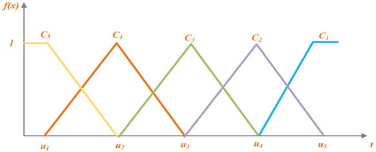
Figure 1.
Membership function.
- (4)
- Construction of the fuzzy comprehensive judgment matrix R
Once the membership function is determined, the membership degree can be obtained based on the measured value. The value is between 0 and 1, and it helps eliminate the dimensional influence of different indicators in the comprehensive evaluation. These values form a fuzzy comprehensive judgment matrix R, as expressed as [36]:
where Ri represents a fuzzy comprehensive judgment matrix.
- (5)
- Comprehensive evaluation
The evaluation sets of the surrounding rock B are obtained on the basis of the weight set of evaluation indicators CW and the fuzzy evaluation matrix. The process is shown as follows [36]:
where CWi represents the comprehensive weight, and i = 1, 2, 3, 4, 5.
The traditional criterion of maximum membership degree will sometimes fail, resulting in unreasonable results. Therefore, this study proposes an improvement by using the confidence identification criterion to obtain the stability of the surrounding rock. It is expressed as:
where k = 1, 2, …, 5 and .
3. Surrounding Rock Stability Evaluation System
3.1. Selection and Principle of Evaluation Indexes
The selection of assessment factors is important for obtaining accurate classification results [37]. Therefore, some principles should be observed:
- (1)
- Comprehensiveness and independence
The evaluation indicators should comprehensively reflect the factors affecting the stability of surrounding rock while selecting significant, largely independent, and representative indicators. This simplifies and enhances the effectiveness of the calculation.
- (2)
- Feasibility
Considering the numerous and complex monitoring and experimental data, the selected evaluation indicators should be practical, operable, and easy to investigate, collect, or measure. This ensures smooth progress in the evaluation process.
- (3)
- Scientificity and reliability
As the purpose of classifying surrounding rock is to reduce the occurrence of risk accidents, ensuring the scientific reliability of the evaluation indicators is essential.
According to the previous research [38], and considering the specific project situation of the project, five factors are selected in accordance with the aforementioned principles [39]. The rock quality designation (RQD), uniaxial compressive strength (Rw), integrality coefficient of the rock mass (KV), strength coefficient of the structural surface (Kf), and groundwater seepage (W) were selected as evaluation indicators for the classification system. A brief introduction is as follows:
- Rock quality designation (I1)
The RQD is the ratio of the cumulative length of intact columnar core samples greater than 10 cm per feed to the feed of each drill return (expressed as a percentage). RQD reflects the degree of rock integrity and is widely used in many rock stability evaluation methods, such as the RMR method and Q method, as expressed by Equation (27).
- 2.
- Uniaxial compressive strength (I2)
It is an important parameter that reflects the mechanical properties of rock. This index has been used as an evaluation index by the Q method and the RMR method, and other methods, so it is used for the study of the classification of the surrounding rock in this paper. It is shown as follows:
where P and A represent the applied load and cross-sectional area of the sample, respectively.
- 3.
- Integrality coefficient of rock mass (I3)
It is a quantitative physical indicator used to assess rock integrity and is widely used for classifying engineering rock masses. It is defined as:
where Vpr and Vpm represent the p-wave velocities of the rock and rock mass (m/s), respectively.
- 4.
- Strength coefficient of structural surface (I4)
Various forms of structural faces are observed in a rock mass, and the integrity of these structural faces is assessed on the basis of a combination of characteristics that can affect the stability of the surrounding rock.
- 5.
- Groundwater seepage (I5)
Groundwater can cause damage to the properties of rock, and its presence or absence differs between dry and water-rich environments [40]. Therefore, understanding the state of groundwater is essential for analyzing the surrounding rock stability.
3.2. Classification of Rock Stability
This study defines the surrounding rock stability according to pertinent literature and other methods (Table 2) in order to achieve a more precise categorization [41,42,43].
Table 2.
Surrounding rock stability classification of other methods.
Various classification methods, as listed in Table 2, divide rock stability into five grades, although six grades or nine grades are also used. To ensure comparability with other methods, this study chooses to classify rock stability into five classes: I, I, II, IV, and V.
3.3. Evaluation System
The surrounding rock stability is classified into five grades, ranging from grade I (excellent rock quality) to grade V (very poor rock quality). Each evaluation index is categorized on the basis of its impact on surrounding rock stability in accordance with different grades [44] (Table 3).
Table 3.
Classification criteria for various indicators of surrounding rock stability.
Based on the above studies, an evaluation system was constructed. It consists of two layers: the first layer represents the stability of the surrounding rock (target layer), and the second layer consists of five indicators (indicator layer).
4. Engineering Case Analysis
4.1. Engineering Background
The Guangzhou Pumped Storage Power Station is a major energy project in South China. The reservoir’s normal storage level of the reservoir is 816.80 m, with a maximum dam height of 68 m and a total reservoir capacity of 24 million km3. The water diversion and power generation system’s pipeline has a total length of approximately 4407 m. The underground plant’s dimensions are 152 m × 22 m × 46 m, and the vault elevation is approximately 239.9 m. Six samples of underground caverns in different parts of the study area were selected (Figure 2).
4.2. Subjective Weights Analysis
Weight seriously affects the accuracy of the results. In this study, IAHP is used to obtain the subjective weights. The procedure is as follows: an expert was invited to assess the interval number of each two indexes through the 1–9 scale to form an interval number evaluation matrix A (Table 4).
Table 4.
Interval number matrix of five factors.

Figure 2.
Surrounding rock data: (a) I1, I2, I5; (b) I3, I4.
Figure 2.
Surrounding rock data: (a) I1, I2, I5; (b) I3, I4.

For example, the interval number of I1 to I3 is [3, 5], which indicates that the expert considers the importance of the two indicators to range between moderately important and strongly important. The interpretation of other interval numbers follows a similar pattern.
The contrast matrix A can be divided into two independent matrices and . After the judgment matrix is constructed, the weight vector can be calculated. The weight vectors and for each matrix using the eigenvalue method through Equations (2) and (3) were calculated, resulting in [0.085, 0.142, 0.110, 0.307, 0.356] T and [0.150, 0.172, 0.111, 0.246, 0.321] T, respectively.
Correction coefficients and for and can be obtained using Equations (4) and (5). In this case, = 0.99 < 1 and = 1.014 > 1, indicating that the weight calculation is qualified by the consistency test. And the subjective weight of each factor can be obtained using Equation (7), as expressed in Table 5.
Table 5.
Results of subjective weight.
After calculation, the subjective weight of each index is [0.117, 0.157, 0.110, 0.277, 0.339] T. The weights are sorted as follows: I5 > I4 > I2 > I1 > I3. It means that the surrounding rock stability is most significantly influenced by groundwater.
4.3. Objective Weights Analysis
Using six samples of surrounding data in the study area, the OW of each index (Table 6) is obtained by Equations (8)–(12).
Table 6.
Objective weight of each index.
After calculation, the objective weight of each index is [0.131, 0.265, 0.173, 0.152, 0.279] T. The weights are sorted as follows: I5 > I2 > I3 > I4 > I1. This indicates that groundwater has the greatest influence on the surrounding rock stability based on the measured data.
4.4. Comprehensive Weights Analysis
After calculating SW and CW, the comprehensive weight can be obtained. and are obtained using Equation (15) in Python, resulting in , and . The calculation is correct. The comprehensive weight is obtained by Equations (16) and (17), resulting in [0.120, 0.175, 0.121, 0.255, 0.329] T.
The weights are sorted as follows: I5 > I4 > I2 > I3 > I1. This indicates that groundwater has the greatest influence on the surrounding rock stability based on the opinion of experts and the data in the study area. The weights are compared in Figure 3 to better visualize the differences between SW, OW, and CW.

Figure 3.
Comparison of different weights.
Analysis of weight results shows that the determination of subjective weights depends on the knowledge of experts, which is highly subjective and arbitrary. The determination of objective weights depends on field-measured data or monitoring data, which is highly objective but lacks human participation and may not fully reflect the actual project situation. Both subjective and objective weights have their shortcomings. Therefore, integrating the characteristics of both and conducting comprehensive empowerment is necessary to reflect experts’ subjective judgment and the objective importance of parameters.
In this study, comprehensive weights are obtained by integrating the SW and OW calculated using IAHP and CV through game theory, resulting in a more reasonable and accurate weight distribution that aligns with the actual situation.
4.5. Comprehensive Fuzzy Evaluation Analysis
In this section, the index and evaluation set, along with the membership functions and evaluation results, are calculated. The membership function serves to transform the index set into the evaluation set, assigning a membership degree between 0 and 1. A higher membership degree indicates a stronger association of the index with a certain level, whereas a lower degree indicates a weaker association [45].
In this study, trapezoidal and trigonometric membership functions (Figure 4) are used to determine the membership degrees.


Figure 4.
Membership degree of each evaluation index. (a) RQD; (b) Rw; (c) Kv; (d) Kf; (e) W.
After determining the membership degree function, the membership degrees are calculated using Equations (20)–(22). The index membership degrees at different levels are obtained by inputting the measured data into the membership degree function, forming a fuzzy matrix. Only a portion of the fuzzy matrix for samples 1, 2, 3, and 5 is shown in Table 7 due to space limitations.
Table 7.
Fuzzy matrix of samples 1, 2, 3, and 5.
The CW is [0.120, 0.175, 0.121, 0.255, 0.329] T. In addition, the evaluation matrix Bi can be obtained using Equation (13). The calculations of four examples are given below:
The calculation of other Bi values follows a similar approach.
5. Results and Discussion
Table 8.
Rock stability grade of six samples.
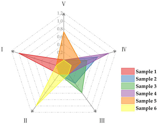
Figure 5.
Results of each sample.
Table 8 and Figure 5 show that the rock stability grades for the samples are I, IV, III, IV, V, and II, respectively. The selection of samples covers a range of surrounding rock stability grades ranging from I to V, indicating that each sample is representative, and the correct determination of multiple samples enhances the reasonability.
The rock stability grades are determined using the confidence criterion of 0.55. For sample 2, the sum of the membership degrees (0 + 0 + 0.290 + 0.710) is 1, which is greater than 0.55. Given that k = 4, the rock stability grade of sample 2 is determined to be IV. For sample 3, the sum of the membership degrees (0 + 0 + 0.582) is greater than 0.55, and k = 3, so the rock stability grade of sample 2 is III. For sample 5, the sum of the membership degrees (0 + 0 + 0 + 0.284 + 0.716) is 1, which is greater than 0.55. Given that k = 5, the rock stability grade of sample 5 is V. The surrounding rock stability grades for the other sections can be obtained in a similar manner. Samples 1 and 6 are determined to be I and II, respectively, indicating good quality of the surrounding rock with no need for additional measures. Samples 2, 3, 4, and 5 are determined to be IV, III, IV, and V, respectively, indicating poor quality. Reinforcement measures, such as bolt support, should be taken.
The relationship between the weight and results of some samples is analyzed using single-factor sensitivity. The weights of each indicator are adjusted by ±5%, ±10%, and ±20% to study their impact on rock stability. Taking sample 2 as an example, the stability of sample 2 show remains the same, that is, grade III, when the weight of factor I5 is reduced by 5%. When the weight is reduced by 10% and 20%, the stability grade is from III to IV. This shows that factor I5 has a greater influence on the stability of the surrounding rock compared with the other indexes. Similar analyses can be performed for other samples.
The results obtained using the proposed method are compared with the uncertainty measure method (UM) [46] and the TOPSIS method [47] to verify its validity and reliability. The comparison results are presented in Table 9 and Figure 6.
Table 9.
Comparison of different methods.

Figure 6.
Comparison of results from different methods.
Figure 6 shows that the results obtained by different methods differ for different samples. The UM method yields results that match the actual levels for samples 2, 4, and 6, and the TOPSIS method’s results match the actual levels for samples 1, 3, 4, and 6. The TOPSIS method calculates the closeness degree to determine the surrounding rock stability, and the result may fall between two grades, making it difficult to obtain an accurate result. The uncertainty measure method determines the stability using attribute measure values, which involves constructing a nonlinear attribute measure function that can be complicated and prone to large calculation errors. The proposed method is simple to calculate and provides accurate and quick results for surrounding rock stability, making it suitable for practical engineering. Field investigations have confirmed that the results of six samples agree with the actual situation. Therefore, the proposed method demonstrates higher precision, and its application to practical projects is feasible compared with the UM method and TOPSIS method.
Although the method presented in this study has been successfully applied in practical projects, it is worth noting that it still has some shortcomings and limitations:
- (1)
- The number of selected sections in the study area is relatively small. Selecting a large number of sections for analysis is recommended to further validate the proposed model;
- (2)
- The use of three different methods to calculate weights has improved the robustness of the weights. However, the subjective influence is difficult to avoid when constructing a judgment matrix in the IAHP.
In future research, more in-depth research will be conducted to address these limitations
6. Conclusions
In this study, an improved FCEM is proposed to evaluate the stability of surrounding rock and provide guidance for safety control in practical engineering. Some conclusions are as follows:
- (1)
- On the basis of the analysis of the actual situation and previous studies, five evaluation indicators are selected: the rock quality designation (RQD), uniaxial compressive strength (Rw), integrality coefficient of the rock mass (KV), strength coefficient of the structural surface (Kf), and groundwater seepage (W). These indicators form the evaluation system for surrounding rock stability, which is categorized into five grades on the basis of the varying influence of each factor on the stability;
- (2)
- The comprehensive weights are determined using a combination of subjective weights through the IAHP and objective weights through CV analysis. The application of game theory helps in obtaining more reasonable and accurate weight distributions for the indicators. Subsequently, an improved FCEM is established, incorporating trapezoidal and triangular membership degree functions to determine the membership degree of each index at different levels. The traditional identification criteria of the model are improved, and the surrounding rock stability grade is determined using confidence criteria;
- (3)
- The proposed model is applied to six sections in an actual project. Comparative analysis with other methods demonstrates that the model provides more accurate and efficient evaluations of the rock stability in different sections. The results of the model are consistent with the field investigations, confirming its rationality and practical value for underground engineering construction and design.
Author Contributions
Conceptualization, X.M.; Methodology, X.M.; Formal analysis, M.W. and R.Z.; Investigation, F.W. and R.Z.; Writing—original draft preparation, X.M. and A.H.; Writing—review and editing, X.M. and A.H. All authors have read and agreed to the published version of the manuscript.
Funding
This study received funding from the Talent Introduction Key Projects of Xihua University (Grant No. Z17112), Graduate Education Teaching Reform and Practice Key Project of Xihua University (Grant No. TJG202303), the Undergraduate Education Reform Program of Xihua University (Grant No. xjjg2019066), and the Natural Science Foundation of Sichuan Province (Grant No. 2022NSFSC1009).
Institutional Review Board Statement
Not applicable.
Informed Consent Statement
Not applicable.
Data Availability Statement
Not applicable.
Acknowledgments
The authors gratefully appreciate the support from Xihua University. The authors would like to express appreciation to the reviewers who helped to improve the quality of the paper.
Conflicts of Interest
The authors declare no conflict of interest.
Nomenclature
| Symbol | Description |
| Interval Judgment matrix | |
| Interval number | |
| X | Weight vector |
| Consistency test coefficient | |
| Consistency test coefficient | |
| S | Standard deviation |
| V | Variation coefficient |
| x | Measured value |
| Correction coefficient of weight | |
| F | Factor set |
| E | Evaluation set |
| f | Membership function |
| u | Boundary values of different grades |
| R | Fuzzy comprehensive judgment matrix |
| B | Fuzzy comprehensive result |
| C | Surrounding rock stability grade |
References
- Zhao, J.-W.; Peng, F.-L.; Wang, T.-Q.; Zhang, X.-Y.; Jiang, B.-N. Advances in Master Planning of Urban Underground Space (UUS) in China. Tunn. Undergr. Space Technol. 2016, 55, 290–307. [Google Scholar] [CrossRef]
- Mahdevari, S.; Shahriar, K.; Sharifzadeh, M.; Tannant, D.D. Stability Prediction of Gate Roadways in Longwall Mining Using Artificial Neural Networks. Neural Comput. Appl. 2016, 28, 3537–3555. [Google Scholar] [CrossRef]
- Idris, M.A.; Nordlund, E.; Saiang, D. Comparison of Different Probabilistic Methods for Analyzing Stability of Underground Rock Excavations. Electron. J. Geotech. Eng. 2016, 21, 6555–6585. [Google Scholar]
- Feng, X.-T.; Zhou, Y.-Y.; Jiang, Q. Rock Mechanics Contributions to Recent Hydroelectric Developments in China. J. Rock Mech. Geotech. Eng. 2019, 11, 511–526. [Google Scholar] [CrossRef]
- Zhang, J.; Shi, K.; Majiti, H.; Shan, H.; Fu, T.; Shi, R.; Lu, Z. Study on the Classification and Identification Methods of Surrounding Rock Excavatability Based on the Rock-Breaking Performance of Tunnel Boring Machines. Appl. Sci. 2023, 13, 7060. [Google Scholar] [CrossRef]
- Xiao, P.; Liu, X.; Zhao, B. Experimental Study on Gas Adsorption Characteristics of Coals under Different Protodyakonov’s Coefficient. Energy Rep. 2022, 8, 10614–10623. [Google Scholar] [CrossRef]
- Deere, D.U.; Hendron, A.J.; Patton, F.D.; Cording, E.J. Design Of Surface And Near-Surface Construction in Rock. In ARMA US Rock Mechanics/Geomechanics Symposium; ARMA: Tampa, FL, USA, 1966; p. ARMA-66-0237. [Google Scholar]
- Bieniawski, Z.T. Engineering Classification of Jointed Rock Masses. Civ. Eng. Siviele Ing. 1973, 15, 335–344. [Google Scholar] [CrossRef]
- Barton, N.; Lien, R.; Lunde, J.J.R.M. Engineering Classification of Rock Masses for the Design of Tunnel Support. Rock Mech. 1974, 6, 189–236. [Google Scholar] [CrossRef]
- Wu, L.; Li, S.; Zhang, M.; Zhang, L. A New Method for Classifying Rock Mass Quality Based on MCS and TOPSIS. Environ. Earth Sci. 2019, 78, 199. [Google Scholar] [CrossRef]
- Wang, Y.; Zhao, N.; Jing, H.; Meng, B.; Yin, X. A Novel Model of the Ideal Point Method Coupled with Objective and Subjective Weighting Method for Evaluation of Surrounding Rock Stability. Math. Probl. Eng. 2016, 2016, 8935156. [Google Scholar] [CrossRef]
- Ren, Y.; Li, T.; Xiong, G.; Lin, Z. New Surrounding Rock Classification Method for High Geostress Tunnels and its Applications. J. Eng. Geol. 2012, 20, 66–73. [Google Scholar]
- Liang, H.R.; Wang, Y.D.; Peng, H.; Liu, J.F.; Yan, X. Classification of Soft Surrounding Rock of Tunnel Based on Normal Cloud Theory. J. Chongqing Jiaotong Univ. 2021, 40, 82–87. [Google Scholar]
- Huang, D.; Li, W.; Chang, X.; Tan, Y. Key Factors Identification and Risk Assessment for the Stability of Deep Surrounding Rock in Coal Roadway. Int. J. Environ. Res. Public Heal. 2019, 16, 2802. [Google Scholar] [CrossRef] [PubMed]
- Liang, M.; Fu, C.; Xiao, B.; Luo, L.; Wang, Z. A Fractal Study for the Effective Electrolyte Diffusion through Charged Porous Media. Int. J. Heat Mass Transf. 2019, 137, 365–371. [Google Scholar] [CrossRef]
- Liang, M.; Liu, Y.; Xiao, B.; Yang, S.; Wang, Z.; Han, H. An Analytical Model for the Transverse Permeability of Gas Diffusion Layer with Electrical Double Layer Effects in Proton Exchange Membrane Fuel Cells. Int. J. Hydrog. Energy 2018, 43, 17880–17888. [Google Scholar] [CrossRef]
- Long, G.; Liu, Y.; Xu, W.; Zhou, P.; Zhou, J.; Xu, G.; Xiao, B. Analysis of Crack Problems in Multilayered Elastic Medium by a Consecutive Stiffness Method. Mathematics 2022, 10, 4403. [Google Scholar] [CrossRef]
- Santos, A.; Lana, M.; Pereira, T. Evaluation of Machine Learning Methods for Rock Mass Classification. Neural Comput. Appl. 2022, 34, 4633–4642. [Google Scholar] [CrossRef]
- Liu, K.; Liu, B.; Fang, Y. An Intelligent Model Based on Statistical Learning Theory for Engineering Rock Mass Classification. Bull. Eng. Geol. Environ. 2019, 78, 4533–4548. [Google Scholar] [CrossRef]
- Ding, Y.; Zhang, W.; Yu, L.; Lu, K. The Accuracy and Efficiency of GA and PSO Optimization Schemes on Estimating Reaction Kinetic Parameters of Biomass Pyrolysis. Energy 2019, 176, 582–588. [Google Scholar] [CrossRef]
- Xu, Z.H.; Li, S.C.; Li, L.P.; Hou, J.G.; Sui, B.; Shi, S.S. Risk Assessment of Water or Mud Inrush of Karst Tunnels Based on Analytic Hierarchy. Process Rock Soil Mech. 2011, 32, 1757–1766. [Google Scholar]
- Saaty, T.; Tran, L. On the Invalidity of Fuzzifying Numerical Judgments in the Analytic Hierarchy Process. Math. Comput. Model. 2007, 46, 962–975. [Google Scholar] [CrossRef]
- Sun, J.; Han, Y.; Li, Y.; Zhang, P.; Liu, L.; Cai, Y.; Li, M.; Wang, H. Construction of a Near-Natural Estuarine Wetland Evaluation Index System Based on Analytical Hierarchy Process and Its Application. Water 2021, 13, 2116. [Google Scholar] [CrossRef]
- Ouma, Y.O.; Tateishi, R. Urban Flood Vulnerability and Risk Mapping Using Integrated Multi-Parametric AHP and GIS: Methodological Overview and Case Study Assessment. Water 2014, 6, 1515–1545. [Google Scholar] [CrossRef]
- Zhang, Y.; Zhang, F.; Zhu, H.; Guo, P. An Optimization-Evaluation Agricultural Water Planning Approach Based on Interval Linear Fractional Bi-Level Programming and IAHP-TOPSIS. Water 2019, 11, 1094. [Google Scholar] [CrossRef]
- Yang, Y.; Chen, G.; Wang, D. A Security Risk Assessment Method Based on Improved FTA-IAHP for Train Position System. Electronics 2022, 11, 2863. [Google Scholar] [CrossRef]
- Huang, R.; Tian, Z.; Lv, Y. Research on Consistency of Reciprocal Judgment Matrix of Interval Rough Numbers. Fuzzy Syst. Math. 2019, 33, 124–133. [Google Scholar]
- Yao, J. Research on Risk Assessment of CTCS-3 Train Control System; Lanzhou Jiaotong University: Lanzhou, China, 2020. [Google Scholar]
- Zang, Z.; Huang, X.; Zhang, Q.; Jiang, C.; Wang, T.; Shang, J.; He, C.; Wan, F. Evaluation of the Effect of Ultrasonic Pretreatment on Vacuum Far-Infrared Drying Characteristics and Quality of Angelica Sinensis Based on Entropy Weight-Coefficient of Variation Method. J. Food Sci. 2023, 88, 1905–1923. [Google Scholar] [CrossRef]
- Zhang, L.; Zhang, X.; Wu, J.; Zhao, D.; Fu, H. Rockburst Prediction Model Based on Comprehensive Weight and Extension Methods and Its Engineering Application. Bull. Eng. Geol. Environ. 2020, 79, 4891–4903. [Google Scholar] [CrossRef]
- Wu, Y.; Deng, Z.; Tao, Y.; Wang, L.; Liu, F.; Zhou, J. Site Selection Decision Framework for Photovoltaic Hydrogen Production Project Using BWM-CRITIC-MABAC: A Case Study in Zhangjiakou. J. Clean. Prod. 2021, 324, 129233. [Google Scholar] [CrossRef]
- Sun, L.; Liu, Y.; Zhang, B.; Shang, Y.; Yuan, H.; Ma, Z. An Integrated Decision-Making Model for Transformer Condition Assessment Using Game Theory and Modified Evidence Combination Extended by D Numbers. Energies 2016, 9, 697. [Google Scholar] [CrossRef]
- Quan, H.; Li, S.; Wei, H.; Hu, J. Personalized Product Evaluation Based on GRA-TOPSIS and Kansei Engineering. Symmetry 2019, 11, 867. [Google Scholar] [CrossRef]
- Li, J.; Deng, C.C.C.; Xu, J.; Ma, Z.; Shuai, P.; Zhang, L. Safety Risk Assessment and Management of Panzhihua Open Pit (OP)-Underground (UG) Iron Mine Based on AHP-FCE, Sichuan Province, China. Sustainability 2023, 15, 4497. [Google Scholar] [CrossRef]
- Shi, S.; Li, S.; Li, L.; Zhou, Z.; Wang, J. Advance Optimized Classification and Application of Surrounding Rock Based on Fuzzy Analytic Hierarchy Process and Tunnel Seismic Prediction. Autom. Constr. 2014, 37, 217–222. [Google Scholar] [CrossRef]
- Cao, J.; He, B.; Qu, N.; Zhang, J.; Liu, C.; Liu, Y.; Chen, C.-L. Benefits Evaluation Method of an Integrated Energy System Based on a Fuzzy Comprehensive Evaluation Method. Symmetry 2023, 15, 84. [Google Scholar] [CrossRef]
- Wang, M.; Xu, X.; Li, J.; Jin, J.; Shen, F. A Novel Model of Set Pair Analysis Coupled with Extenics for Evaluation of Surrounding Rock Stability. Math. Probl. Eng. 2015, 2015, 892549. [Google Scholar] [CrossRef]
- Ma, J.; Li, T.; Li, X.; Zhou, S.; Ma, C.; Wei, D.; Dai, K. A Probability Prediction Method for the Classification of Surrounding Rock Quality of Tunnels with Incomplete Data Using Bayesian Networks. Sci. Rep. 2022, 12, 19846. [Google Scholar] [CrossRef]
- Xue, Y.; Li, Z.; Qiu, D.; Zhang, L.; Zhao, Y.; Zhang, X.; Zhou, B. Classification Model for Surrounding Rock Based on the PCA-Ideal Point Method: An Engineering Application. Bull. Eng. Geol. Environ. 2019, 78, 3627–3635. [Google Scholar] [CrossRef]
- Wu, Y.; Qiao, W.; Li, Y.; Jiao, Y.; Zhang, S.; Zhang, Z.; Liu, H. Application of Computer Method in Solving Complex Engineering Technical Problems. IEEE Access 2021, 9, 60891–60912. [Google Scholar] [CrossRef]
- GB/T 50218-94; National Standard of the People’s Republic of China. Standard for Engineering Classification of Rock Masses. China Building Industry Press: Beijing, China, 1995.
- JTG D70-2004; Industrial Standard of the People’s Republic of China. Code for Design of Road Tunnel. China Communications Press: Beijing, China, 2004.
- GB 50021-2001; National Standard of the People’s Republic of China. Code for Investigation of Geotechnical Engineering. China Building Industry Press: Beijing, China, 2002.
- Wu, S.; Yang, S.; Du, X. A Model for Evaluation of Surrounding Rock Stability Based on D-S Evidence Theory and Error-Eliminating Theory. Bull. Eng. Geol. Environ. 2021, 80, 2237–2248. [Google Scholar] [CrossRef]
- He, S.; Song, D.; Mitri, H.; He, X.; Chen, J.; Li, Z.; Xue, Y.; Chen, T. Integrated Rockburst Early Warning Model Based on Fuzzy Comprehensive Evaluation Method. Int. J. Rock Mech. Min. Sci. 2021, 142, 104767. [Google Scholar] [CrossRef]
- He, H.; Yan, Y.; Qu, C.; Fan, Y. Study and Application on Stability Classification of Tunnel Surrounding Rock Based on Uncertainty Measure Theory. Math. Probl. Eng. 2014, 2014, 626527. [Google Scholar] [CrossRef]
- Gu, X.-B.; Ma, Y.; Wu, Q.-H.; Liu, Y.-B. The Application of Intuitionistic Fuzzy Set-TOPSIS Model on the Level Assessment of the Surrounding Rocks. Shock. Vib. 2022, 2022, 4263276. [Google Scholar] [CrossRef]


Disclaimer/Publisher’s Note: The statements, opinions and data contained in all publications are solely those of the individual author(s) and contributor(s) and not of MDPI and/or the editor(s). MDPI and/or the editor(s) disclaim responsibility for any injury to people or property resulting from any ideas, methods, instructions or products referred to in the content. |
© 2023 by the authors. Licensee MDPI, Basel, Switzerland. This article is an open access article distributed under the terms and conditions of the Creative Commons Attribution (CC BY) license (https://creativecommons.org/licenses/by/4.0/).