Dynamical Behaviors in a Stage-Structured Model with a Birth Pulse

Abstract

This paper presents an exploitation model with a stage structure to analyze the dynamics of a fish population, where periodic birth pulse and pulse fishing occur at different fixed time. By utilizing the stroboscopic map, we can obtain an accurate cycle of the system and investigate the stability thresholds. Through the application of the center manifold theorem and bifurcation theory, our research has shown that the given model exhibits transcritical and flip bifurcation near its interior equilibrium point. The bifurcation diagrams, maximum Lyapunov exponents and phase portraits are presented to further substantiate the complexity. Finally, we present high-resolution stability diagrams that demonstrate the global structure of mode-locking oscillations. We also describe how these oscillations are interconnected and how their complexity unfolds as control parameters vary. The two parametric planes illustrate that the structure of Arnold’s tongues is based on the Stern–Brocot tree. This implies that the periodic occurrence of birth pulse and pulse fishing contributes to the development of more complex dynamical behaviors within the fish population.

1. Introduction

Many scholars have extensively discussed the optimal management of renewable resources, which is directly related to sustainable development [1,2,3,4]. The phenomenon of instantaneous population change in the development and utilization of biological resources is very common. For example, many fish populations are seasonal breeders, resulting in a rapid increase in the number of fry over a short period of time. As the world’s marine fisheries are struggling with the serious issue of overexploitation, direct overfishing poses a clear and present danger to their survival. It is highly realistic for decision makers to devise a workable scheme that sustains fisheries at a high level of productivity and meets economic needs [5,6]. There are two key factors in fisheries, namely, the effect of the seasonality and population stage-structure [7,8,9]. Impulsive differential Equations (hybrid dynamical system) provide a natural way to describe such phenomena.

The impulsive differential equations have been widely studied and have seen significant progress in recent years by many authors [10,11,12,13]. It has found widespread application in a variety of fields, including biological technology, medicine dynamics, physics, economy, population dynamics, and epidemiology [14]. It is widely accepted that both natural and human-induced phenomena can have impulsive effects on population dynamics and epidemiology.

The theory of impulsive differential equations was introduced by Mil’man and Mishkis [15] in the 1960s and has since undergone rapid development [16,17,18]. This theory provides a good description for real-world processes involving abrupt changes at certain time intervals. The most commonly encountered types of impulsive differential equations found in the mathematical literatures are instantaneous impulses, non-instantaneous impulses and autonomous impulsive Equations [19,20]. Nevertheless, as previously mentioned, almost all authors have utilized ODE, delay ODE or impulsive ODE models to investigate biological systems. Various models can be used to describe diverse biological phenomena, each with its own unique strengths. Certain species, such as numerous insect species, exhibit no temporal overlap between successive generations, and thus, their populations evolve in discrete time-steps. The discrete differential equation model is more suitable for biological systems than continuous model, particularly in situations where populations have a short lifespan and non-overlapping generations in the real world. Therefore, it is reasonable to pursue the study of biological models governed by differential equations, as they provide a powerful tool for understanding complex biological phenomena [21,22]. The purpose of this paper is to explore the dynamic characteristics of a discrete population model with a stage structure.

This paper is split into sections as follows. Section 2 presents the pulse fishing population model with stage structure and birth pulse. In Section 3, we prove the existence and stability of equilibria in this model. Section 4 focuses on the theoretical analysis of transcritical and flip bifurcation. Numerical simulations are provided to illustrate the complex dynamics of the model in Section 5. Finally, Section 6 provides a comprehensive summary of the results and serves as the concluding section for the paper.

2. Single-Species Population Model with Stage Structure

Here, we consider the single-species population model proposed by Gao et al. [23]:

$$\left\{\begin{array}{c}\dot{x}\left(t\right)=\frac{b}{c+N{\left(t\right)}^m}y\left(t\right)-dx\left(t\right)-\delta x\left(t\right),\hfill \\ \dot{y}\left(t\right)=\delta x\left(t\right)-dy\left(t\right),\hfill \end{array}\right.$$

(1)

where $x\left(t\right)$ and $y\left(t\right)$ are the population densities of immature and mature, respectively, $d>0$ represents the constant death rate, the maturity rate is denoted by $\delta (\delta >0)$, which governs the average duration of the juvenile period, $b/(c+N{\left(t\right)}^m)$ is the birth rate of mature population, and $N\left(t\right)=x\left(t\right)+y\left(t\right),x\left(t\right)\in R,y\left(t\right)\in R,b,c,m>0$.

In model (1), we assume that there are different death rates for immature and mature population, denoted as $d_1$ and $d_2$, respectively. In order to account for the harvesting of mature individuals, we propose modifying system (1) in the following manner:

$$\left\{\begin{array}{c}\dot{x}\left(t\right)=\frac{b}{c+N{\left(t\right)}^m}y\left(t\right)-d_{1}x\left(t\right)-\delta x\left(t\right),\hfill \\ \dot{y}\left(t\right)=\delta x\left(t\right)-d_{2}y\left(t\right)-Ey\left(t\right),\hfill \end{array}\right.$$

(2)

where $E(0\le E<1)$ denotes the harvesting effort.

Model (2) has traditionally assumed that the mature population is born continuously throughout the year, whereas in reality, births may be seasonal or occur in regular pulses. Numerous large mammal and fish populations have been observed to exhibit a growth pattern referred to as a "birth pulse" by Gao et al. [23]. In other words, reproduction occurs in a relatively short period each year. Furthermore, we also consider pulse fishing and assume that the time taken to harvest is fixed annually. To further develop the model, we introduce periodic birth and harvesting at different fixed time. Specifically, we will consider a model with a birth pulse and a harvesting pulse:

$$\left\{\begin{array}{cc}\dot{x}\left(t\right)=-d_{1}x\left(t\right)-\delta x\left(t\right),\hfill & \\ \dot{y}\left(t\right)=\delta x\left(t\right)-d_{2}y\left(t\right),\hfill & t\ne n+T,t\ne n+1,\hfill \\ x\left(t^{+}\right)=x\left(t\right),\hfill & \\ y\left(t^{+}\right)=(1-E)y\left(t\right),\hfill & t=n+T,\hfill \\ x\left(t^{+}\right)=x\left(t\right)+\frac{by\left(t\right)}{c+{(x\left(t\right)+y\left(t\right))}^m},\hfill & \\ y\left(t^{+}\right)=y\left(t\right),\hfill & t=n+1,\hfill \end{array}\right.$$

(3)

where $T(0\le T<1)$ is the fishing time after the birth pulse each year and $n\in Z^{+}$.

By performing a series of complex calculations in [23], one can obtain the following stroboscopic map for system (3):

$$\left\{\begin{array}{c}x\to rx+\frac{b(px+qy)}{c+{[(r+p)x+qy]}^m},\hfill \\ y\to px+qy,\hfill \end{array}\right.$$

(4)

where $0<r=e^{-(\delta +d_1)}<1,0<p=\frac{\delta }{\delta +d_1-d_2}[(1-E)e^{-d_2}-e^{-(\delta +d_1)}+E{e}^{-T(\delta +d_1)-(1-T)d_2}],$$0<q=(1-E)e^{-d_2}<1$.

Equation (4) illustrates the numbers of immature and mature individuals in a population at a birth pulse in terms of values from the previous birth pulse. In other words, we are observing the system’s behavior at its pulsing period using stroboscopic sampling. The dynamic behaviors of system (4) will influence the dynamics of system (3). Consequently, in the subsequent section, our analysis will center on system (4) and explore its diverse dynamic behaviors.

3. Existence and Stability of Equilibria

By solving system (4), we can obtain that there exists a trivial equilibrium $E_0(0,0)$, as well as an unique positive equilibrium $E(x_{*},y_{*})$ when $bp>c(1-r)(1-q)$, whose expression can be given by:

$$\left\{\begin{array}{c}{x}_{*}=\frac{1-q}{r(1-q)+p}\sqrt[m]{c(R-1)},\hfill \\ y_{*}=\frac{p}{r(1-q)+p}\sqrt[m]{c(R-1)},\hfill \end{array}\right.$$

(5)

where $R=\frac{bp}{c(1-r)(1-q)}$.

Initially, we will analyze the stability of the fixed points $E_0(0,0)$ and $E(x_{*},y_{*})$. The Jacobian matrix of system (4) at any fixed point can be expressed as:

$$\mathit{J}=\left(\begin{array}{cc}r+\frac{bpG-bm(r+p)(px+qy)H^{m-1}}{G^2}& \frac{bqG-bmq(px+qy)H^{m-1}}{G^2}\\ p& q\end{array}\right),$$

where

$$G=c+{[(r+p)x+qy]}^m,H=(r+p)x+qy.$$

It is evident that the characteristic polynomial of J reads as:

$$F\left(\lambda \right)={\lambda }^2-Tr\left(J\right)\lambda +Det\left(J\right),$$

(6)

where

$$\begin{array}{ccc}& & Tr\left(J\right)=r+q+\frac{bpG-bm(r+p)y_{*}{H}^{m-1}}{G^2},\hfill \\ & & Det\left(J\right)=rq-\frac{bmrq{y}_{*}{H}^{m-1}}{G^2}.\hfill \end{array}$$

By using Jury conditions in [24], we can assert that $E_0(0,0)$ is asymptotically stable provided that $b<c(1-r)(1-q)/p$. Our next objective is to explore the stability analysis of the unique positive equilibrium $E(x_{*},y_{*})$.

In order to study the local stability and bifurcation phenomenon of the positive equilibrium, the following lemma will be very useful and essential, which can be demonstrated conveniently by examining the relationship between roots and coefficients of a quadratic Equation [25,26].

Lemma 1.

Let $F\left(\lambda \right)={\lambda }^2+P\lambda +Q$, and $F\left(1\right)>0$. Suppose ${\lambda }_1$ and ${\lambda }_2$ are two roots of $F\left(\lambda \right)=0$. Then, the following results hold true:

(i) 

$|{\lambda }_1| < 1$ and $|{\lambda }_2| < 1$⇔$F(-1) > 0$ and $Q < 1$;

(ii) 

$|{\lambda }_1| > 1$ and $|{\lambda }_2| > 1$⇔$F(-1) > 0$ and $Q > 1$;

(iii) 

$|{\lambda }_1| < 1$ and $|{\lambda }_2| > 1$ (or $|{\lambda }_1| > 1$ and $|{\lambda }_2| < 1$) ⇔$F(-1) < 0$.

(iv) 

${\lambda }_1,{\lambda }_2$ are complex and $|{\lambda }_1|=|{\lambda }_2|=1$⇔$P^2-4Q < 0$ and $Q=1$.

By applying Lemma 1 and some definitions in [25,26], the following conclusions can be obtained.

Theorem 1.

The interior fixed point $E(x_{*},y_{*})$ fulfills the following conditions:

1. 

E is a sink if and only if $b>\frac{-(1+r)(1+q)G^2}{pG-m{y}_{*}(r+p+qr)H^{m-1}},b<\frac{(rq-1)G^2}{mrq{y}_{*}{H}^{m-1}}.$

2. 

E is a source if and only if $b>\frac{-(1+r)(1+q)G^2}{pG-m{y}_{*}(r+p+qr)H^{m-1}},b>\frac{(rq-1)G^2}{mrq{y}_{*}{H}^{m-1}}.$

3. 

E is a saddle if and only if $b<\frac{-(1+r)(1+q)G^2}{pG-m{y}_{*}(r+p+qr)H^{m-1}}.$

4. 

E is non-hyperbolic if one of the following conditions is true:

(1) 

$b=\frac{(1-r)(1-q)G^2}{pG-m{y}_{*}(r+p-rq)H^{m-1}}$ and $b\ne b_1^{*}=\frac{-(r+q)G^2}{pG-m(r+p)y_{*}{H}^{m-1}},b\ne b_2^{*}=\frac{(2-r-q)G^2}{pG-m(r+p)y_{*}{H}^{m-1}}$;

(2) 

$b=\frac{-(1+r)(1+q)G^2}{pG-m{y}_{*}(r+p+qr)H^{m-1}}$ and $b\ne \frac{-(r+q)G^2}{pG-m(r+p)y_{*}{H}^{m-1}},b\ne \frac{(2-r-q)G^2}{pG-m(r+p)y_{*}{H}^{m-1}}$.

In the non-hyperbolic case, equilibrium can lead to bifurcations and chaos. From the above conclusion, if the condition (4.1) is met, one eigenvalue of E is 1, and the other is $-1+q+r+\frac{bpG-bm(r+p)y_{*}{H}^{m-1}}{G^2}\ne -1,1$, namely there exists a transcritical bifurcation. If the condition (4.2) is satisfied, it can be easily observed that one of the eigenvalues of E is $-1$, and the other is $1+q+r+\frac{bpG-bm(r+p)y_{*}{H}^{m-1}}{G^2}\ne -1,1$, that is to say, a flip bifurcation will occur. Now, let us define the following two sets:

$$\begin{array}{ccc}& & T_B=\left\{(b,c,p,r,m,q)\in R_{+}^6:b=\overline{b}=\frac{(1-r)(1-q)G^2}{pG-m{y}_{*}(r+p-rq)H^{m-1}},b\ne b_1^{*},b_2^{*}\right\},\hfill \\ & & F_B=\left\{(b,c,p,r,m,q)\in R_{+}^6:b=\tilde{b}=\frac{-(1+r)(1+q)G^2}{pG-m{y}_{*}(r+p+rq)H^{m-1}},b\ne b_1^{*},b_2^{*}\right\},\hfill \end{array}$$

at which transcritical bifurcation and flip bifurcation will appear, respectively.

4. Bifurcation Analysis

In this section, the possible bifurcation scenarios at the unique equilibrium $E(x_{*},y_{*})$ for system (4) will be investigated based on the analysis presented in Section 3.

4.1. Transcritical Bifurcation at E

To begin with, we analyze the transcritical bifurcation at E. From Theorem 1, it is straightforward to determine that two eigenvalues of $J\left(E\right)$ are ${\lambda }_1=1,{\lambda }_2\ne \pm 1$. It is important to note that all parameters are located within the set $T_B$, and b fluctuates in a vicinity of $T_B$. Consequently, the point $E(x_{*},y_{*})$ passes through a transcrtical bifurcation.

Choose b as a bifurcation parameter, and assume $u=x-x_{*},v=y-y_{*},b_{*}=b-\overline{b}$. In this case, the fixed point E is shifted to the origin, the system (2.4) is perturbed into:

$$\left[\begin{array}{c}u\\ v\end{array}\right]\to \left[\begin{array}{cc}{a}_{11}& a_{12}\\ p& q\end{array}\right]\left[\begin{array}{c}u\\ v\end{array}\right]+\left[\begin{array}{c}f(u,v)+O\left(\right|u,v{|}^4)\\ 0\end{array}\right],$$

(7)

where

$$\begin{array}{ccc}& & f(u,v)=a_1{u}^2+a_{2}uv+a_3{v}^2+a_4{u}^3+a_5{u}^{2}v+a_{6}u{v}^2+a_7{v}^3+b_{1}u{b}_{*}+b_{2}v{b}_{*},\hfill \\ & & +b_3{u}^2{b}_{*}+b_{4}uv{b}_{*}+b_5{v}^2{b}_{*},\hfill \end{array}$$

with:

$$\begin{array}{ccc}& & a_{11}=r+\frac{bpG-bm(r+p)y_{*}{H}^{m-1}}{G^2},a_{12}=\frac{bqG-bmq{y}_{*}{H}^{m-1}}{G^2},\hfill \\ & & a_1=\frac{b{m}^2{(r+p)}^2{y}_{*}{H}^{2m-2}}{G^3}-\frac{bm(r+p)H^{m-2}[2pH+(m-1)(r+p)y_{*}]}{2G^2},\hfill \\ & & a_2=\frac{2bq{m}^2(p+r)y_{*}{H}^{2m-2}}{G^3}-\frac{bmq{H}^{m-2}[(r+p)(m-1)y_{*}+2pH+rH]}{G^2},\hfill \\ & & a_3=\frac{b{y}_{*}{m}^2{q}^2{H}^{2m-2}}{G^3}-\frac{bm{q}^2{H}^{m-2}[2H+(m-1)y_{*}]}{2G^2},\hfill \\ & & a_4=\frac{-b{y}_{*}{m}^3{(p+r)}^3{H}^{3m-3}}{G^4}+\frac{b{m}^2{(p+r)}^2{H}^{2m-3}[(m-1)(p+r)y_{*}+pH]}{G^3}\hfill \\ & & -\frac{bm(m-1){(p+r)}^2{H}^{m-3}[(m-2)(p+r)y_{*}+3pH]}{6G^2},\hfill \\ & & a_5=\frac{-3bq{y}_{*}{m}^3{(p+r)}^2{H}^{3m-3}}{G^4}+\frac{bq{m}^2(r+p)H^{2m-3}[3pH+rH+3(m-1)(p+r)y_{*}]}{G^3}\hfill \\ & & -\frac{bqm(m-1)(r+p)H^{m-3}[3pH+rH+(m-2)(p+r)y_{*}]}{2G^2},\hfill \\ & & a_6=\frac{-3b{y}_{*}{q}^2{m}^3(p+r)H^{3m-3}}{G^4}+\frac{b{q}^2{m}^2{H}^{2m-3}[3pH+2rH+3(m-1)(p+r)y_{*}]}{G^3}\hfill \\ & & -\frac{bm{q}^2(m-1)H^{m-3}[3pH+2rH+(m-2)(p+r)y_{*}]}{2G^2},\hfill \\ & & a_7=\frac{3b{m}^2{q}^3{H}^{2m-3}[H+(m+1)y_{*}]}{G^3}-\frac{bm{q}^3(m-1)H^{m-3}[y_{*}(m-2)+3H]}{6G^2}\hfill \\ & & -\frac{b{y}_{*}{q}^3{m}^3{H}^{3m-3}}{G^4},b_1=\frac{pG-m(r+p)y_{*}{H}^{m-1}}{G^2},b_2=\frac{qG-mq{y}_{*}{H}^{m-1}}{G^2},\hfill \\ & & b_3=\frac{m^2{(r+p)}^2{y}_{*}{H}^{2m-2}}{G^3}-\frac{m(r+p)H^{m-2}[2pH+(m-1)(p+r)y_{*}]}{2G^2},\hfill \\ & & b_4=\frac{2q(r+p)m^2{y}_{*}{H}^{2m-2}}{G^3}-\frac{mq{H}^{m-2}[2pH+rH+(m-1)(p+r)y_{*}]}{G^2},\hfill \\ & & b_5=\frac{m^2{q}^2{y}_{*}{H}^{2m-2}}{G^3}-\frac{m{q}^2{H}^{m-2}[2H+(m-1)y_{*}]}{2G^2}.\hfill \end{array}$$

Make a non-singular linear coordinate transformation:

$$\left[\begin{array}{c}u\\ v\end{array}\right]=\left[\begin{array}{cc}\frac{a_{12}}{1-a_{11}}& \frac{a_{12}}{q-1}\\ 1& 1\end{array}\right]\left[\begin{array}{c}X\\ Y\end{array}\right].$$

(8)

Then, the map (4.1) becomes:

$$\left[\begin{array}{c}X\\ Y\end{array}\right]\to \left[\begin{array}{cc}1& 0\\ 0& q+a_{11}-1\end{array}\right]\left[\begin{array}{c}X\\ Y\end{array}\right]+\left[\begin{array}{c}f(X,Y,b_{*})+O\left(\right|X,Y,b_{*}{|}^4)\\ g(X,Y,b_{*})+O\left(\right|X,Y,b_{*}{|}^4)\end{array}\right],$$

(9)

where

$$\begin{array}{ccc}& & f(X,Y,b_{*})=\frac{p}{2-q-a_{11}}\sum _{2\le j+k+l\le 3}{f}_{jkl}{X}^j{Y}^k{b}_{*}^l,g(X,Y,b_{*})=-f(X,Y,b_{*}),\hfill \\ & & f_{020}=\frac{a_1{a}_{12}^2}{{(q-1)}^2}+\frac{a_2{a}_{12}}{q-1}+a_3,f_{110}=\frac{-2a_1{a}_{12}}{p}-\frac{a_2(q-a_{11})}{p}+2a_3,\hfill \\ & & f_{200}=\frac{a_1{a}_{12}^2}{{(1-a_{11})}^2}+\frac{a_2{a}_{12}}{1-a_{11}}+a_3,f_{030}=\frac{a_4{a}_{12}^3}{{(q-1)}^3}+\frac{a_5{a}_{12}^2}{{(q-1)}^2}+\frac{a_6{a}_{12}}{q-1}+a_7,\hfill \\ & & f_{120}=-\frac{3a_4{a}_{12}^2}{p(q-1)}+\frac{a_5{a}_{12}^2}{{(q-1)}^2}-\frac{2a_5{a}_{12}}{p}+\frac{a_6{a}_{12}}{1-a_{11}}+\frac{2a_6{a}_{12}}{q-1}+3a_7,\hfill \\ & & f_{210}=-\frac{3a_4{a}_{12}^2}{p(1-a_{11})}+\frac{a_5{a}_{12}^2}{{(1-a_{11})}^2}-\frac{2a_5{a}_{12}}{p}+\frac{2a_6{a}_{12}}{1-a_{11}}+\frac{a_6{a}_{12}}{q-1}+3a_7,\hfill \\ & & f_{300}=\frac{a_4{a}_{12}^3}{{(1-a_{11})}^3}+\frac{a_5{a}_{12}^2}{{(1-a_{11})}^2}+\frac{a_6{a}_{12}}{1-a_{11}}+a_7,f_{011}=\frac{b_1{a}_{12}}{q-1}+b_2,\hfill \\ & & f_{101}=\frac{b_1{a}_{12}}{1-a_{11}}+b_2,f_{111}=\frac{b_4{a}_{12}}{q-1}+\frac{b_4{a}_{12}}{1-a_{11}}-\frac{2b_3{a}_{12}}{p}+2b_5,\hfill \\ & & f_{021}=\frac{b_3{a}_{12}^2}{{(q-1)}^2}+\frac{b_4{a}_{12}}{q-1}+b_5,f_{201}=\frac{b_3{a}_{12}^2}{{(1-a_{11})}^2}+\frac{b_4{a}_{12}}{1-a_{11}}+b_5.\hfill \end{array}$$

To discuss the stability of $(X,Y)=(0,0)$ near $b_{*}=0$, consider the following center manifold:

$$W^C(0,0,0)=\{(X,Y,b_{*})\in R^3|Y=h(X,b_{*}),h(0,0)=0,Dh(0,0)=0\},$$

where X and $b_{*}$ are sufficiently small. Suppose that:

$$Y=h_1{X}^2+h_2{b}_{*}^2+h_{3}X{b}_{*}+O\left(\right|X,b_{*}{|}^3).$$

It is not difficult to calculate:

$$h_1=-\frac{g_{200}}{q+a_{11}-2},h_2=0,h_3=-\frac{g_{101}}{q+a_{11}-2}.$$

Consequently, the system (9) restricted to the center manifold is described by:

$$\begin{array}{ccc}& & X\to f(X,b_{*})=X+\frac{p{f}_{200}}{2-q-a_{11}}{X}^2+\frac{p{f}_{101}}{2-q-a_{11}}X{b}_{*}+O\left(\right|X,b_{*}{|}^3).\hfill \end{array}$$

Then, we have:

$$\begin{array}{ccc}& & f(0,0)=0,\frac{\partial f}{\partial X}(0,0)=1,\frac{\partial f}{\partial b_{*}}(0,0)=0,\hfill \\ & & \frac{{\partial }^{2}f}{\partial X\partial b}(0,0)=\frac{p{f}_{101}}{2-q-a_{11}},\frac{{\partial }^{2}f}{\partial X^2}(0,0)=\frac{2p{f}_{200}}{2-q-a_{11}}.\hfill \end{array}$$

According to the conclusions in [27], all necessary conditions hold for a transcritical bifurcation to occur. Finally, we arrive at the following conclusions regarding the direction and existence of the transcritical bifurcation.

Theorem 2.

Suppose $(b,m,r,p,q,c)\in T_B$. There exists a transcritical bifurcation at $E(x_{*},y_{*})$ when $f_{101}\ne 0$, $f_{200}\ne 0$ and the parameter b deviates within a small neighborhood of $\overline{b}$.

4.2. Flip Bifurcation at E

In this section, by applying the center manifold theorem and bifurcation theory in [24,25,26,27], we investigate the flip bifurcation at $E(x_{*},y_{*})$.

When $b=\tilde{b}$, the two eigenvalues of J are ${\lambda }_1=-1,{\lambda }_2\ne \pm 1$, and the fixed point $E(x_{*},y_{*})$ sustains flip bifurcation whenever the parameters deviate within the small neighborhood of $F_B$. Choose b as a bifurcation parameter, and assume $u=x-x_{*},v=y-y_{*}$. Then, the fixed point E is shifted to the origin, and system (2.4) is devoted to:

$$\left[\begin{array}{c}u\\ v\end{array}\right]\to \left[\begin{array}{cc}{a}_{11}& a_{12}\\ p& q\end{array}\right]\left[\begin{array}{c}u\\ v\end{array}\right]+\left[\begin{array}{c}f(u,v)+O\left(\right|u,v{|}^4)\\ 0\end{array}\right],$$

(10)

where the expression of $f(u,v)$ can be found in model (4.1) by replacing $b=\tilde{b}+b_{**}$.

For the conversion of coefficient matrix J into a normal form, we use the following translation:

$$\left[\begin{array}{c}u\\ v\end{array}\right]=\left[\begin{array}{cc}{a}_{12}& a_{12}\\ -1-a_{11}& {\lambda }_2-a_{11}\end{array}\right]\left[\begin{array}{c}X\\ Y\end{array}\right].$$

(11)

From Equations (10) and (11), it follows that:

$$\left[\begin{array}{c}X\\ Y\end{array}\right]\to \left[\begin{array}{cc}-1& 0\\ 0& {\lambda }_2\end{array}\right]\left[\begin{array}{c}X\\ Y\end{array}\right]+\left[\begin{array}{c}\overline{f}(X,Y,b_{**})+O\left(\right|X,Y,b_{**}{|}^4)\\ \overline{g}(X,Y,b_{**})+O\left(\right|X,Y,b_{**}{|}^4)\end{array}\right],$$

(12)

where

$$\begin{array}{ccc}& & \overline{f}(X,Y,b_{**})=\frac{{\lambda }_2-a_{11}}{a_{12}(1+{\lambda }_2)}[a_1{u}^2+a_{2}uv+a_3{v}^2+a_4{u}^3+a_5{u}^{2}v+a_{6}u{v}^2+a_7{v}^3\hfill \\ & & +b_{1}u{b}_{**}+b_{2}v{b}_{**}+b_3{u}^2{b}_{**}+b_{4}uv{b}_{**}+b_5{v}^2{b}_{**}],\hfill \\ & & \overline{g}(X,Y,b_{**})=\frac{1+a_{11}}{a_{12}(1+{\lambda }_2)}[a_1{u}^2+a_{2}uv+a_3{v}^2+a_4{u}^3+a_5{u}^{2}v+a_{6}u{v}^2+a_7{v}^3\hfill \\ & & +b_{1}u{b}_{**}+b_{2}v{b}_{**}+b_3{u}^2{b}_{**}+b_{4}uv{b}_{**}+b_5{v}^2{b}_{**}],\hfill \\ & & u=a_{12}(X+Y),v=-(1+a_{11})X+({\lambda }_2-a_{11})Y.\hfill \end{array}$$

By the center manifold theory, the stability of the equilibrium can be assessed by analyzing a one-parameter family of map on a center manifold $W^C\left(0\right)$, which can be written as:

$$W^C\left(0\right)=\{(X,Y,b_{**})\in R^3:Y=h_1{X}^2+h_{2}X{b}_{**}+h_3{b}_{**}^2\}.$$

On the basis of the invariance of the center manifold, we have:

$$\begin{array}{ccc}& & h_1=\frac{a_{12}(1+a_{11})a_1}{1-{\lambda }_2^2}-\frac{a_2{(1+a_{11})}^2}{1-{\lambda }_2^2}+\frac{a_3{(1+a_{11})}^3}{a_{12}(1-{\lambda }_2^2)},\hfill \\ & & h_2=\frac{(1+a_{11})[b_1{a}_{12}-b_2(1+a_{11})]}{1-{\lambda }_2^2},h_3=0.\hfill \end{array}$$

Therefore, the map (12) restricted to the center manifold is referred to as:

$$F:X\to -X+k_1{X}^2+k_{2}X{b}_{**}+k_3{X}^2{b}_{**}+k_{4}X{b}_{**}^2+k_5{X}^3+O\left(\right|X,b_{**}{|}^4),$$

where

$$\begin{array}{ccc}& & k_1=\frac{a_{12}({\lambda }_2-a_{11})a_1}{1+{\lambda }_2}-\frac{({\lambda }_2-a_{11})(1+a_{11})a_2}{1+{\lambda }_2}+\frac{({\lambda }_2-a_{11}){(1+a_{11})}^2{a}_3}{a_{12}(1+{\lambda }_2)},\hfill \\ & & k_2=\frac{({\lambda }_2-a_{11})a_{12}{b}_1-({\lambda }_2-a_{11})(1+a_{11})b_2}{a_{12}(1+{\lambda }_2)},\hfill \\ & & k_3=\frac{2a_{12}{h}_2({\lambda }_2-a_{11})a_1}{1+{\lambda }_2}+\frac{{({\lambda }_2-a_{11})}^2{a}_2{h}_2}{1+{\lambda }_2}+\frac{({\lambda }_2-a_{11})a_{12}{b}_3}{1+{\lambda }_2}+\frac{({\lambda }_2-a_{11})h_1{b}_1}{1+{\lambda }_2}\hfill \\ & & -\frac{2{({\lambda }_2-a_{11})}^2(1+a_{11})a_3{h}_2}{a_{12}(1+{\lambda }_2)}-\frac{({\lambda }_2-a_{11})(1+a_{11})a_2{h}_2}{1+{\lambda }_2}-\frac{({\lambda }_2-a_{11})(1+a_{11})b_4}{1+{\lambda }_2}\hfill \\ & & +\frac{({\lambda }_2-a_{11}){(1+a_{11})}^2{b}_5}{a_{12}(1+{\lambda }_2)}+\frac{{({\lambda }_2-a_{11})}^2{h}_1{b}_2}{a_{12}(1+{\lambda }_2)},\hfill \\ & & k_4=\frac{({\lambda }_2-a_{11})b_1{h}_2}{1+{\lambda }_2}+\frac{{({\lambda }_2-a_{11})}^2{b}_2{h}_2}{a_{12}(1+{\lambda }_2)},\hfill \\ & & k_5=\frac{({\lambda }_2-a_{11})a_{12}^2{a}_4}{1+{\lambda }_2}-\frac{({\lambda }_2-a_{11})(1+a_{11})a_{12}{a}_5}{1+{\lambda }_2}+\frac{2({\lambda }_2-a_{11})a_{12}{h}_1{a}_1}{1+{\lambda }_2}\hfill \\ & & +\frac{({\lambda }_2-a_{11}){(1+a_{11})}^2{a}_6}{1+{\lambda }_2}-\frac{({\lambda }_2-a_{11})(1+a_{11})a_2{h}_1}{1+{\lambda }_2}+\frac{{({\lambda }_2-a_{11})}^2{a}_2{h}_1}{1+{\lambda }_2}\hfill \\ & & -\frac{({\lambda }_2-a_{11}){(1+a_{11})}^3{a}_7}{a_{12}(1+{\lambda }_2)}-\frac{2(1+a_{11}){({\lambda }_2-a_{11})}^2{a}_3{h}_1}{a_{12}(1+{\lambda }_2)}.\hfill \end{array}$$

Owing to the aforementioned computation, two non-zero real numbers are defined as:

$${\alpha }_1=\frac{({\lambda }_2-a_{11})b_1}{1+{\lambda }_2}-\frac{({\lambda }_2-a_{11})(1+a_{11})b_2}{a_{12}(1+{\lambda }_2)},{\alpha }_2=k_1^2+k_5,$$

which are the existence conditions for flip bifurcation.

In summary, the above analysis indicates that a flip bifurcation of system (2.4) occurs at the positive equilibrium E and that the stability of the period orbits is contingent upon the value of ${\alpha }_2$. As a result, we have the following implications.

Theorem 3.

As a result, a flip bifurcation exists around $E(x_{*},y_{*})$ whenever b deviates within a small neighborhood of $\tilde{b}$ and ${\alpha }_{1,2}\ne 0$. Additionally, if ${\alpha }_2>0({\alpha }_2<0)$, then the period-two orbits that bifurcated from E are stable (unstable).

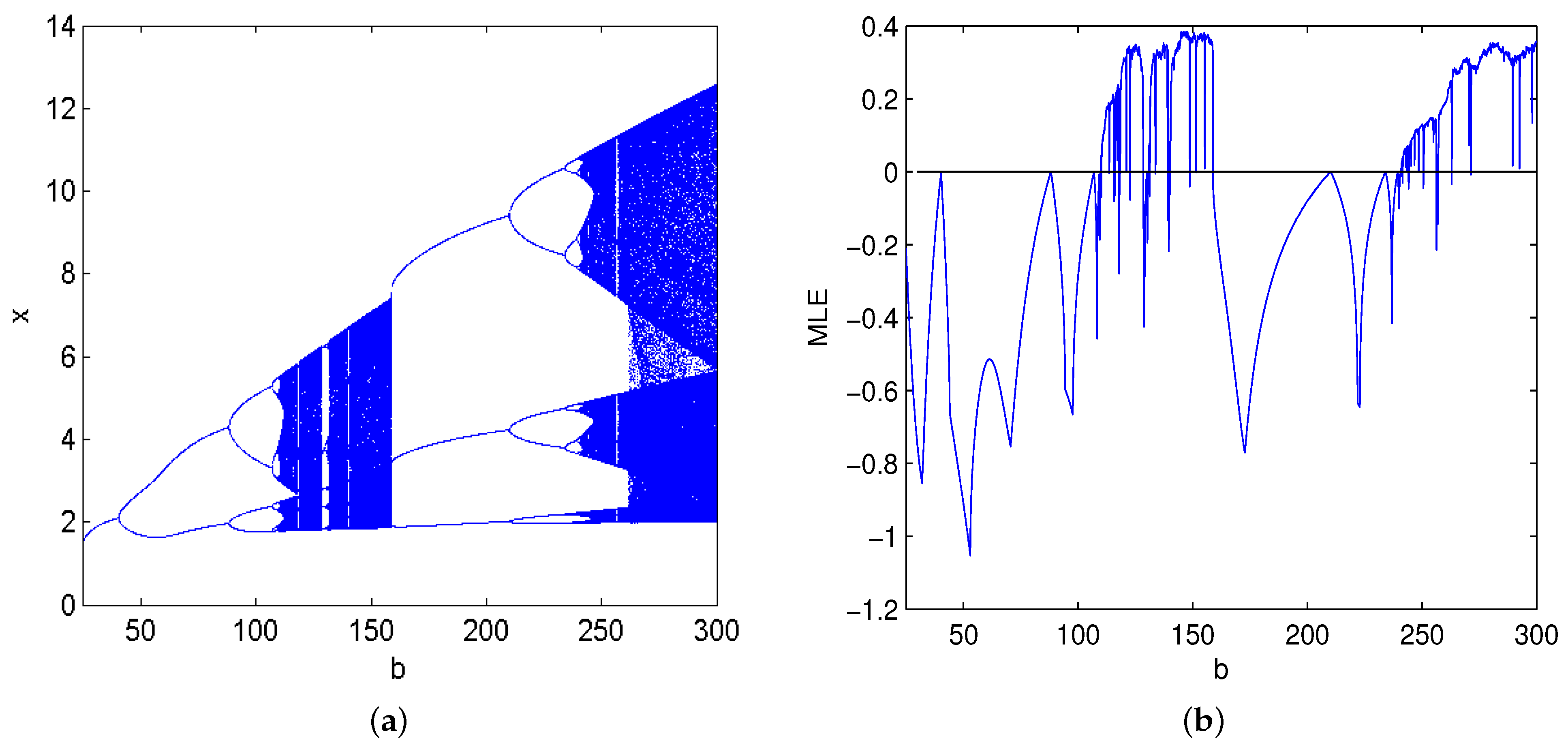
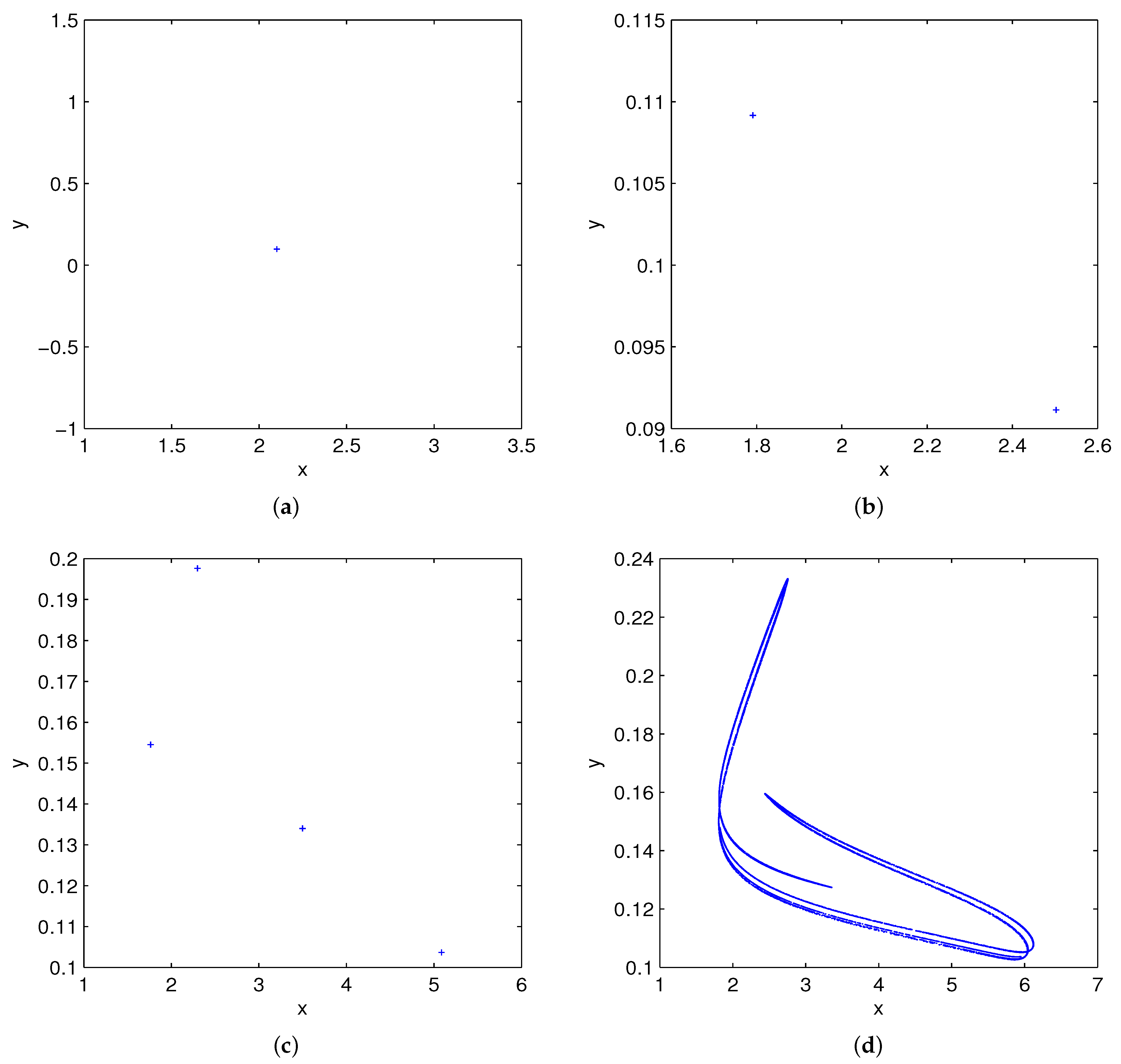
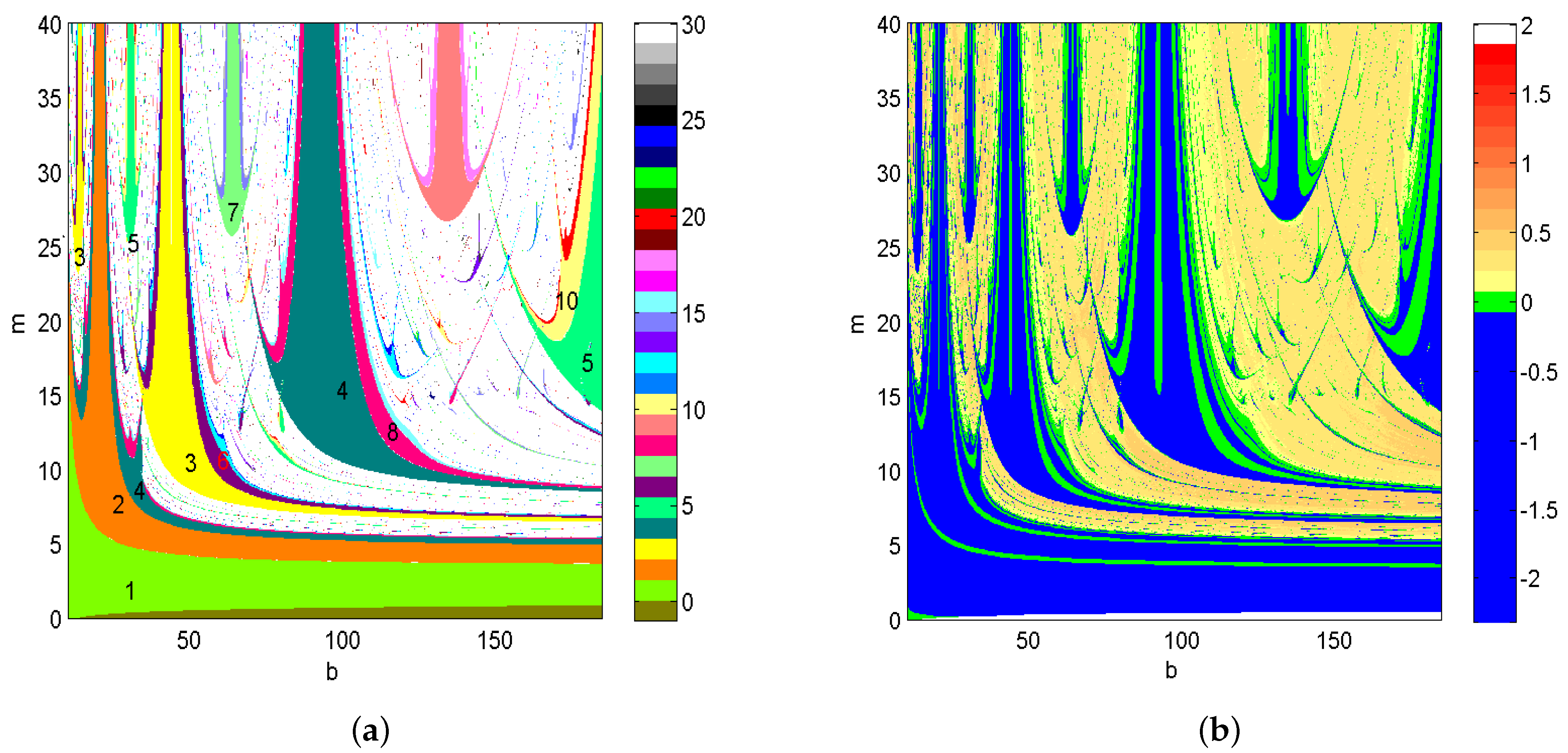
5. Numerical Simulations

A bifurcation diagram [28,29] is an effective tool for analyzing the dynamic behaviors of different attractors with a changing parameter. To gain a rudimentary comprehension of the dynamics of system (2.4), a one-dimensional bifurcation diagram has been computed, as illustrated in Figure 1. To substantiate the occurrence of flip bifurcation, we select a set of parameters as $T=0.25,E=0.6,c=2,\delta =0.2,d_1=0.6,d_2=0.3,m=8$.

Figure 1a illustrates that b is stable for $b<40.62$, and a flip bifurcation occurs when $b=40.62$. As b exceeds $b=124$, it traverses a series of bifurcations that ultimately result in chaotic dynamics. Subsequently, periodic motion and chaotic motion alternate in succession. In Figure 1b, we demonstrate the powerful Lyapunov exponent test [30] to confirm the periodic motion and chaotic motion. As can be seen from it, when $25<b<124$, the system exhibits regular motion; when $124<b<162$, it routes to chaotic motion, and so on. This is in accordance with the phenomena observed in Figure 1a, which is the focus of our analysis.

The phase portraits for different b values are employed to determine the nature of the bifurcation that causes the system to evolve into chaos. The phase portraits in Figure 2 show that there are orbits of period 1, 2, and 4 when $b=40$, $b=80$, and $b=100$, respectively. Meanwhile, Figure 2d displays the system as chaotic for $b=124$.

Next, we utilize two types of high-resolution stability phase diagrams to uncover novel kinetics in the system (2.4). Figure 3a represents isoperiodic diagram of the $(b,m)$ parameter-space for system (2.4) with $T=0.25,E=0.6,c=2,\delta =0.2,d_1=0.6,d_2=0.3$. A colorbar with 30 colors is employed to illustrate the number of periods. For example, a period-3 solution is depicted in yellow, a period-29 solution is shown in light gray, and the regions for periods 2–28 are distinguished using various colors and marked with distinct numbers. In addition to periodic solutions, quasiperiodic solutions and chaotic solutions are plotted in white. It is necessary to note that the identification of quasi-periodic regions goes beyond the scope of determining the number of periods. Instead, we use Lyapunov phase diagrams (shown in Figure 3b), which are complementary to phase diagrams in Figure 3a, to identify these regions. The colorbar on the right of Figure 3b is linked to the magnitude of the largest Lyapunov exponent. The periodic motion is illustrated using a gradual dark green-light blue scale. The green area represents the quasiperiodic response, while a continuously light yellow to dark red region signifies the chaotic motion. It is clear that the dynamic responses predicted by Figure 3a,b are in good agreement with each other, despite being generated in different methods.

Figure 3a provides a detailed depiction of various Arnold tongues, which are arranged in a regular pattern based on a small and incomplete portion of the Stern–Brocot sum tree [31,32]. For instance, the period-2 tongue (father) contains two period-3 tongues (daughters) on either side, with each daughter tongue having its own two daughter tongues of period-4 and period-5. Evidently, the aforementioned construction rule also applies to the subsequent period-4 and period-5 tongues. A tongue with a longer period can also be derived through the fractal self-similarity of the structure, which is not unwound to evade repetition. While generating the aforementioned tongues, we observed that the sequence of periodicities corresponds perfectly to the integers in the Stern–Brocot sum tree as the control parameters were adjusted. These distinctive and regular trees are presented in Figure 2 in [31], which can be obtained from the Stern–Brocot tree by summing the numerator and denominator of the fractions. Moreover, in some overlapping regions, various periodic, quasi-periodic, and chaotic responses can be observed. Within these quasi-periodic phases, the boundaries of each Arnold tongue are loci of period doubling (flip) bifurcations. This suggests that there are numerous period-adding cascades present in the discrete model.

As previously mentioned, the observations of well-organized trees depicted above may offer a closed formula to explain the intricate patterns underlying non-linear systems. In other words, it has become possible to investigate the tongues with higher periods in model (2.4), since their periods follow a regular pattern based on the Stern–Brocot sum tree. This pattern can be also found in the parameter-space $(E,m)$ and $(T,m)$ depicted in Figure 4.

6. Conclusions

To summarize, we have conducted a comprehensive analysis of the bifurcations for a discrete-time model with both birth and harvesting pulses. Our theoretical findings indicate that the impulsive system undergoes transcritical and flip bifurcations. In order to construct the bifurcation diagrams for these cases, normal forms for maps and their approximations to the flows of the corresponding differential equations are utilized. Numerical simulation results, including bifurcation diagrams, Maximum Lyapunov Exponents, and phase portraits, are employed to demonstrate fascinating dynamical behaviors. Furthermore, the phase diagrams with high quality are employed to demonstrate the mode-locking structures. Our study also reveals the appearance of Stern–Brocot trees in this pulsing system. We anticipate that the Stern–Brocot tree will prove to be a highly versatile categorization tool for mode-locking oscillations of the impulsive system.

References

1. Tang, S.Y.; Chen, L.S. The effect of seasonal harvesting on stage-structured population models. J. Math. Biol. 2003, 48, 357–374. [Google Scholar] [CrossRef]
2. Battistelli, C.; Baringo, L.; Conejo, A. Optimal energy management of small electric energy systems including V2G facillities and renewable energy sources. Electr. Pow. Syst. Res. 2012, 92, 50–59. [Google Scholar] [CrossRef]
3. Murty, V.V.; Kumar, A. Optimal energy managemet and technoeconomic analysis in microgrid with hybrid renewable energy source. J. Mod. Power. Syst. Clean Energy 2020, 8, 929–940. [Google Scholar] [CrossRef]
4. Kesavan, T.; Lakshmi, K. Optimization of a renewable energy source-based virtual power plant for electrical energy management in an unbalanced distribution network. Sustainability 2022, 14, 11129. [Google Scholar] [CrossRef]
5. Ben Miled, S.; Kebir, A.; Hbid, M.L. Mathematical Modeling Describing the Effect of Fishing and Dispersion on Hermaphrodite Population Dynamics. Int. Rev. Red. Cross 2010, 5, 159–179. [Google Scholar] [CrossRef]
6. Arino, O.; Hbid, M.L.; Bravo de la Parra, R. A mathematical model of growth of population of fish in the larval stage: Density-dependence effects. Math. Biosci. 1998, 150, 1–20. [Google Scholar] [CrossRef]
7. Gao, S.J.; Chen, L.S. The effect of seasonal harvesting on a single-species discrete population model with stage structure and birth pulses. Chaos Solitons Fract. 2005, 24, 1013–1023. [Google Scholar] [CrossRef]
8. Liu, J.L.; Zhang, T.L. Global dynamics of a stage-structured hantavirus infection model with seasonality. Nonlinear. Anal. 2021, 26, 21–40. [Google Scholar] [CrossRef]
9. Soudijin, F.H.; de Roos, A.M. Approximation of a physiologically structured population model with seasonal reproduction by a stage-structured biomass mdel. Theor. Ecol. 2017, 10, 73–90. [Google Scholar] [CrossRef]
10. Kaul, S.K.; Liu, X.Z. Generalized variation of parameters and stability of impulsive system. Nonlinear. Anal. 2000, 40, 295–307. [Google Scholar] [CrossRef]
11. Raheem, A. Oscillation criteria for impulsive partial fractional differential equations. Comput. Math. Appl. 2017, 107, 17–21. [Google Scholar] [CrossRef]
12. Church, K.E.M. Eigenvalues and delay differential equations: Periodic coefficients, impulses and rigorous numerics. J. Dyn. Diff. Equ. 2021, 33, 2173–2252. [Google Scholar] [CrossRef]
13. Xia, M.L.; Liu, L.N.; Fang, J.Y.; Zhang, Y.C. Stability analysis for a class of stochastic differential equations with impulses. Mathematics 2023, 11, 1542. [Google Scholar] [CrossRef]
14. Feketa, P.; Klinshov, V.; Lucken, L. A survey on the modeling of hybrid behaviors: How to account for impulsive jumps properly. Commun. Nonlinear Sci. 2021, 103, 105955. [Google Scholar] [CrossRef]
15. Milman, V.D.; Myshkis, A.D. On the stability of motion in the presence of impulses. Sib. Math. J. 1960, 1, 233–237. [Google Scholar]
16. Bainov, D.D.; Minchev, E.; Nakagawa, K. Asymptotic behaviour of solutions of impulsive semilinear parabolic equations. Nonlinear Anal. 1997, 30, 2725–2734. [Google Scholar] [CrossRef]
17. Liu, X.N.; Chen, L.S. Global dynamics of the periodic logistic system with periodic impulsive perturbations. J. Math. Anal. Appl. 2004, 289, 279–291. [Google Scholar] [CrossRef] [Green Version]
18. Ma, Y.; Liu, B.; Feng, W. Dynamics of a birth-pulse single-species model with restricted toxin input and pulse harvesting. Discret. Dyn. Nat. Soc. 2010, 2010, 142534. [Google Scholar] [CrossRef] [Green Version]
19. Samoilenko, A.M.; Perestyuk, A.A. Impulsive Differential Equations; World Scientific: Singapore, 1995. [Google Scholar]
20. Hernández, E.; O’Regan, D. On a new class of abstract impulsive differential equations. Proc. Am. Math. Soc. 2013, 141, 1641–1649. [Google Scholar]
21. Lindner, F.; Schilling, R.L. Weak order for the discretization of the stochastic heat equation driven by impulsive noise. Potential. Anal. 2013, 38, 345–379. [Google Scholar] [CrossRef] [Green Version]
22. Liu, B.; Wu, R.C. Bifurcation and patterns analysis for a spatiotemporal discrete Gierer-Meinhart system. Mathematics 2022, 10, 243. [Google Scholar] [CrossRef]
23. Gao, S.J.; Chen, L.S.; Sun, L.H. Optimal pulse fishing policy in stage-structured models with birth pulses. Chaos Solitons Fract. 2005, 25, 1209–1219. [Google Scholar] [CrossRef]
24. Kuznetsov, Y.A. Elements of Applied Bifurcation Theory, 2nd ed.; Springer: New York, NY, USA, 1988. [Google Scholar]
25. Liu, X.J.; Liu, Y.; Chu, Y.D. Bifurcation and chaos in a host-parasitoid model with a lower bound for the host. Adv. Differ. Equ. 2018, 2018, 31. [Google Scholar] [CrossRef] [Green Version]
26. Yousef, A.; Yousef, F.B. Bifurcation and stability analysis of a system of fractional-order differential equations for a plant-herbivore model with Allee effect. Mathematics 2019, 7, 454. [Google Scholar] [CrossRef] [Green Version]
27. Singh, A.; Sharma, V.S. Bifurcations and chaos control in a discrete-time prey-predator model with Holling type-II functional response and prey huge. J. Comput. Appl. Math. 2023, 418, 114666. [Google Scholar] [CrossRef]
28. Tang, S.Y.; Chen, L.S. Chaos in functional response host-parasitoid ecosystem models. Chaos Solitons Fract. 2002, 13, 875–884. [Google Scholar] [CrossRef]
29. Lv, S.J.; Zhao, M. The dynamic complexity of a host-parasitoid model with a lower bound for the host. Chaos Solitons Fract. 2008, 36, 911–919. [Google Scholar] [CrossRef]
30. Magnitskii, N.A. Universal bifurcation chaos theory and its new applications. Mathematics 2023, 11, 2536. [Google Scholar] [CrossRef]
31. Rao, X.B.; Chu, Y.D.; Zhang, J.G.; Gao, J.S. Complex mode-locking oscillations and Stern-Brocot derivation tree in a CSTR reaction with impulsive perturbations. Chaos 2020, 30, 113117. [Google Scholar] [CrossRef]
32. Klapcsik, K.; Varga, R.; Hegeds, F. Bi-parameter topology of subharmonics of an asymmetric bubble oscillator at high dissipation rate. Nonlinear Dyn. 2018, 94, 2373–2389. [Google Scholar] [CrossRef]
Figure 1. (a) Flip Bifurcation of map (2.4) in ( b , x ) space. (b) The Maximum Lyapunov Exponent (MLE) related to (a).
Mathematics 11 03321 g001
Figure 2. The phase trajectory for (a) b = 40 , (b) b = 80 , (c) b = 100 , (d) b = 124 .
Mathematics 11 03321 g002
Figure 3. Two complementary types of stability diagrams in ( b , m ) parameter space. (a) The period stability diagram shows that mode-locking oscillations are regularly organized according to the Stern–Brocot sum tree. (b) The corresponding Lyapunov phase diagram emphasizing quasi-periodic response.
Mathematics 11 03321 g003
Figure 4. Period stability diagrams observed in two additional parameter planes (a) E × m parameter plane, (b) T × m parameter plane.
Mathematics 11 03321 g004
Disclaimer/Publisher’s Note: The statements, opinions and data contained in all publications are solely those of the individual author(s) and contributor(s) and not of MDPI and/or the editor(s). MDPI and/or the editor(s) disclaim responsibility for any injury to people or property resulting from any ideas, methods, instructions or products referred to in the content.