An Exact In-Plane Equilibrium Equation for Transversely Loaded Large Deflection Membranes and Its Application to the Föppl-Hencky Membrane Problem

Abstract

In the existing literature, there are only two in-plane equilibrium equations for membrane problems; one does not take into account the contribution of deflection to in-plane equilibrium at all, and the other only partly takes it into account. In this paper, a new and exact in-plane equilibrium equation is established by fully taking into account the contribution of deflection to in-plane equilibrium, and it is used for the analytical solution to the well-known Föppl-Hencky membrane problem. The power series solutions of the problem are given, but in the form of the Taylor series, so as to overcome the difficulty in convergence. The superiority of using Taylor series expansion over using Maclaurin series expansion is numerically demonstrated. Under the same conditions, the newly established in-plane equilibrium equation is compared numerically with the existing two in-plane equilibrium equations, showing that the new in-plane equilibrium equation has obvious superiority over the existing two. A new finding is obtained from this study, namely, that the power series method of using Taylor series expansion is essentially different from that of using Maclaurin series expansion; therefore, the recurrence formulas for power series coefficients of using Maclaurin series expansion cannot be derived directly from that of using Taylor series expansion.

1. Introduction

The “membrane” is a term in mechanics which refers to a laterally loaded thin plate whose edge displacement is always completely constrained (fixed) during deflection. Therefore, “thin plate bending problems” [1,2,3,4,5] differ from “membrane deflecting problems” [6,7,8,9,10], mainly in that the thin plates under lateral loading undergo both tensile stress and compressive stress in bending problems (i.e., undergoing the so-called bending stresses), and undergo only tensile stress in deflecting problems due to the always fully fixed edge displacements (as if the bending stiffness of the plates vanishes). In general, the large deflection problems of laterally loaded thin plates or membranes are solved analytically by establishing the governing equations such as geometric equations and equilibrium equations, in which the accuracies of these governing equations depend usually on whether the deflection effect is properly taken into account, which further affects the accuracies of the solutions of these large deflection problems. Obviously, the deflections in membrane deflecting problems are usually much greater than that in thin plate bending problems, especially when the inverted deflected circular membranes are used to design the so-called membrane shells or bending-free shells [11,12,13,14,15,16], the desired maximum deflections of the membranes may reach half the radius of the membranes (which is not possible in thin plate bending problems). This means that the deflections in membrane deflecting problems have a greater influence on the establishment of the geometric equations and equilibrium equations, in comparison with the deflections in thin plate bending problems.

The mathematical equations that describe the relationship between strain and displacement in large deflection problems are called geometric equations, and are established usually by studying the spatial geometric relationships between micro straight or curved line elements before and after the deformation. For example, in cylindrical coordinate systems, the radial geometric equation is established by analyzing the spatial geometric relationship between a micro, initially flat, radial (straight) line element before the deformation and its meridional (curved) line element after the deformation with deflection, while the circumferential geometric equation is established by analyzing the spatial geometric relationship between a micro, initially flat, circumferential (curved) line element before the deformation and its circumferential (curved) line element after the deformation with deflection. The classical geometric equations are derived under the assumption of small thin plate or membrane deflections, and only partly take into account the effect of deflections to the spatial geometric relationship, but are widely used [17,18,19,20,21]. Therefore, Lian et al. [22] improved the classical geometric equations and presented the new geometric equations suitable for larger deflection membranes.

The so-called out-of-plane equilibrium equation refers to the mathematical equation describing the equilibrium of the forces perpendicular to the plane in which the geometric middle plane of the initially flat thin plates or membranes is located. By ignoring the terms related to bending stiffness in the Föppl-von Kármán out-of-plane equilibrium equation of thin plates [23,24], Hencky [25] derived an out-of-plane equilibrium equation suitable for the large deflection problem of transversely uniformly loaded circular thin plates with vanishing bending stiffness, i.e., the so-called Föppl-Hencky membrane problem, the large deflection problem of transversely uniformly loaded circular membranes. An incorrect power series coefficient in [25] was corrected by Chien [26] and Alekseev [27], respectively. Sun et al. [28] used the power series method for differential equations to solve the Föppl-Hencky membrane problem, where the out-of-plane equilibrium equation used is essentially the same as that used in [25]. However, the classical Föppl-von Kármán out-of-plane equilibrium equation was actually derived under the assumption of small rotation angles or small deflections. But membranes tend to exhibit very large elastic deflections. Therefore, Sun et al. [29] established a new out-of-plane equilibrium equation suitable for the large deflection Föppl-Hencky membranes.

The classical in-plane equilibrium equation, which was established originally for thin plate bending problems [23,24], is actually applicable only to planar stretching or compressing problems of thin plates or membranes, because it does not take into account the contribution of deflection to in-plane equilibrium at all, i.e., the equilibrium of the forces parallel to the plane in which the geometric middle plane of the initially flat thin plates or membranes is located. But in practice, this classical in-plane equilibrium equation was often used to solve the large deflection problems of thin plates [30,31,32,33,34,35,36,37] or even membranes [38,39,40,41,42,43,44]. It is obvious that these large deflection problems require an in-plane equilibrium equation that takes into account the contribution of deflection to in-plane equilibrium, especially for those membranes that tend to exhibit large elastic deflections. Therefore, Li et al. [45] established an in-plane equilibrium equation suitable for large deflection problems. However, the in-plane equilibrium equation in [45] is observed actually to take into account only the partial contribution of deflection to in-plane equilibrium, which still affects the accuracy of solving those membranes with very large deflections.

In this paper, the contribution of deflection to in-plane equilibrium is fully taken into account, and an exact in-plane equilibrium equation is derived. As an example of application, the derivation of the exact in-plane equilibrium equation is combined with the solution to the well-known Föppl-Hencky membrane problem. In the following section, the Föppl-Hencky membrane problem is reformulated with the derived exact in-plane equilibrium equation, the resulting governing equations are solved by using the power series method and Maclaurin series expansion (see Section 2.6.1) and Taylor series expansion (see Section 2.6.2), and new power series solutions of the problem are presented, where a new finding is obtained, that the power series method of using Taylor series expansion is essentially different from that of using Maclaurin series expansion, and therefore, the recurrence formulas for power series coefficients of using Maclaurin series expansion cannot be derived directly from that of using Taylor series expansion. In Section 3, some important issues are discussed, such as the relationship and essential difference between the power series solutions of using Maclaurin series expansion and Taylor series expansion, the superiority of using Taylor series expansion over using Maclaurin series expansion, the convergence of the obtained power series solutions, and the superiority of the derived exact in-plane equilibrium equation over the classical and previously improved in-plane equilibrium equations. The concluding remarks are shown in Section 4.

2. Membrane Equation and Solution

It should be stated first that in the following reformulation of the well-known Föppl-Hencky membrane problem, all the other governing equations, except the in-plane equilibrium equation, are consistent with those in the references [22,46], in order to facilitate comparison under the same conditions. A uniformly distributed transverse loads q is quasi-statically applied to an initially flat and peripherally fixed circular membrane with radius a, thickness h, Poisson’s ratio ν, and Young’s modulus of elasticity E, resulting in an axisymmetric deformation with large deflection of the circular membrane, as shown in Figure 1, where the dash-dotted line represents the geometric middle plane of the initially flat circular membrane, r, φ, w, and o denote the radial coordinate, circumferential coordinate, transverse coordinate, and original of the introduced cylindrical coordinate system (r, φ, w); also, w denotes the transverse displacement of the circular membrane under the loads q, but the circumferential coordinate φ is not represented in Figure 1 due to the axisymmetric nature of the problem under consideration.

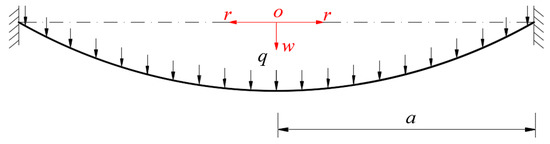
Figure 1. Profile of the deflected circular membrane under the uniformly distributed transverse loads q.

2.1. Formulation of Out-of-Plane Equilibrium Equation

As shown in Figure 2, a free body with radius r (0 ≤ r ≤ a) is taken out from the central portion of the deflected circular membrane in Figure 1 to study the static problem of equilibrium of this free body in the direction perpendicular to the polar plane (r, φ), where σ_r and θ denote the radial stress and rotation angle at any point on the deflected circular membrane, h is the thickness of the circular membrane, and σ_rh is the membrane force acting on the boundary r.

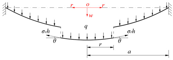
Figure 2. Profile of the free body under the external loads q and the membrane force σ_rh.

Obviously, in the direction perpendicular to the polar plane (r, φ), there are only two vertical forces, i.e., the vertical downward force πr²q, and the vertical upward force 2πrσ_rhsinθ. Therefore, the equilibrium condition in the vertical direction is

$$2\pi r{\sigma }_{r}h\sin \theta -\pi r^{2}q=0.$$

(1)

If the transverse displacement at r is denoted by w, then

$$\sin \theta =1/\sqrt{1+1/{\tan }^2\theta }=1/\sqrt{1+1/{(-\mathrm{d}w/\mathrm{d}r)}^2}.$$

(2)

Substituting Equation (2) into Equation (1), the out-of-plane equilibrium equation may be written as

$$\frac{1}{2}rq\sqrt{1+1/{(-\mathrm{d}w/\mathrm{d}r)}^2}={\sigma }_{r}h.$$

(3)

2.2. Formulation of In-Plane Equilibrium Equation

A micro area element $ABCD$ is taken out arbitrarily from the deflected circular membrane in Figure 1 along the meridional curves $\stackrel{⌢}{AB}$ and $\stackrel{⌢}{DC}$ and circumferential curves $\stackrel{⌢}{AD}$ and $\stackrel{⌢}{BC}$, as shown in Figure 3, where $A^{\prime }{B}^{\prime }{C}^{\prime }{D}^{\prime }$ represents the projection of the micro area element $ABCD$ on the polar plane (r, φ), $\Delta r$ and $\Delta \phi$ are the increments of the radial coordinate r and circumferential coordinate φ, σ_t is the circumferential stress at r, $w_m$ denotes the maximum deflection at the center of the circular membrane (i.e., the deflection w at r = 0), and $\overrightarrow{om}$ is the bisector of the angle $\angle A^{\prime }o{D}^{\prime }$.

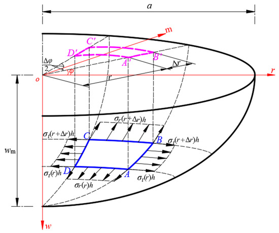
Figure 3. The micro area element ABCD taken out arbitrarily from the deflected circular membrane and its projection A′B′C′D′ on the polar plane (r, φ).

We now deal with the in-plane equilibrium problem of the micro area element $ABCD$ under the joint actions of the radial membrane forces σ_r(r)h and σ_r(r + ∆r)h and circumferential membrane forces σ_t(r)h and σ_t(r + ∆r)h, i.e., the static problem of equilibrium in the direction parallel to the polar plane (r, φ), as shown in Figure 4, where θ(r + ∆r) and θ(r) denote the rotation angles of the deflected circular membrane at the circumferential curves $\stackrel{⌢}{BC}$ and $\stackrel{⌢}{AD}$ in Figure 3, respectively.

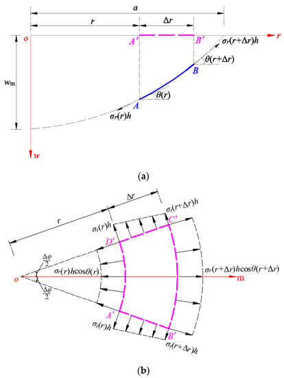
Figure 4. Schematic diagram: (a) The profile, along the meridian in which the curve $\stackrel{⌢}{AB}$ in Figure 3 is located, of the deflected circular membrane; (b) The projection of the radial membrane forces σ_r(r)h and σ_r(r + ∆r)h and circumferential membrane forces σ_t(r)h and σ_t(r + ∆r)h on the polar plane (r, φ).

In the horizontal direction parallel to the polar plane (r, φ), there are four horizontal forces acting on the micro area element $ABCD$; they are the horizontal component ${\sigma }_r(r+\Delta r)h\cos \theta (r+\Delta r)$ of the radial membrane force ${\sigma }_r(r+\Delta r)h$ acting on the boundary $\stackrel{⌢}{BC}$ (corresponding to the projection $\stackrel{⌢}{B^{\prime }{C}^{\prime }}$ on the polar plane (r, φ), see Figure 4), the horizontal component ${\sigma }_r(r)h\cos \theta (r)$ of the radial membrane force ${\sigma }_r(r)h$ acting on the boundary $\stackrel{⌢}{AD}$ (corresponding to the projection $\stackrel{⌢}{A^{\prime }{D}^{\prime }}$ on the polar plane (r, φ), see Figure 4), and the horizontal circumferential membrane forces acting on the boundaries $\stackrel{⌢}{AB}$ and $\stackrel{⌢}{CD}$, which may be approximated by $[{\sigma }_t(r+\Delta r)h+{\sigma }_t(r)h]/2$. Therefore, the condition that the resultant force in the direction of the bisector $\overrightarrow{om}$ is equal to zero yields

$$\begin{array}{l}(r+\Delta r)\Delta \phi \cdot {\sigma }_r(r+\Delta r)h\cdot \cos \theta (r+\Delta r)-r\Delta \phi \cdot {\sigma }_r(r)h\cdot \cos \theta (r)\\ -2\sin \frac{\Delta \phi }{2}\cdot \frac{{\sigma }_t(r)h+{\sigma }_t(r+\Delta r)h}{2}\frac{\Delta r}{\cos \theta (r)}=0\end{array}$$

(4)

Given that $\sin (\Delta \phi /2)\approx \Delta \phi /2$ when $\Delta \phi \to 0$, Equation (4) can, therefore, be reduced to the following form

$$\begin{array}{l}(r+\Delta r)\cdot {\sigma }_r(r+\Delta r)\cdot \cos \theta (r+\Delta r)-r{\sigma }_r(r)\cdot \cos \theta (r)\\ -\frac{{\sigma }_t(r)+{\sigma }_t(r+\Delta r)}{2}\frac{\Delta r}{\cos \theta (r)}=0\end{array}$$

(5)

Let us expand ${\sigma }_r(r+\Delta r)$, ${\sigma }_t(r+\Delta r)$ and $\cos \theta (r+\Delta r)$ into the Taylor series and ignore the higher order terms therein

$${\sigma }_r(r+\Delta r)={\sigma }_r(r)+\frac{\mathrm{d}{\sigma }_r(r)}{\mathrm{d}r}\Delta r+\frac{1}{2!}\frac{{\mathrm{d}}^2{\sigma }_r(r)}{\mathrm{d}{r}^2}{(\Delta r)}^2+\dots \approx {\sigma }_r(r)+\frac{\mathrm{d}{\sigma }_r(r)}{\mathrm{d}r}\Delta r,$$

(6)

$${\sigma }_t(r+\Delta r)={\sigma }_t(r)+\frac{\mathrm{d}{\sigma }_t(r)}{\mathrm{d}r}\Delta r+\frac{1}{2!}\frac{{\mathrm{d}}^2{\sigma }_t(r)}{\mathrm{d}{r}^2}{(\Delta r)}^2+\dots \approx {\sigma }_t(r)+\frac{\mathrm{d}{\sigma }_t(r)}{\mathrm{d}r}\Delta r$$

(7)

and

$$\cos \theta (r+\Delta r)=\cos \theta (r)+\frac{\mathrm{d}\cos \theta (r)}{\mathrm{d}r}\Delta r+\frac{1}{2!}\frac{{\mathrm{d}}^2\cos \theta (r)}{\mathrm{d}{r}^2}{(\Delta r)}^2+\dots \approx \cos \theta (r)+\frac{\mathrm{d}\cos \theta (r)}{\mathrm{d}r}\Delta r.$$

(8)

Substituting Equations (6)–(8) into Equation (5) and taking the limit as $\Delta r\to 0$ yields

$$r\frac{\mathrm{d}{\sigma }_r(r)}{\mathrm{d}r}\cos \theta (r)+{\sigma }_r(r)\cos \theta (r)+r{\sigma }_r(r)\frac{\mathrm{d}\cos \theta (r)}{\mathrm{d}r}-\frac{{\sigma }_t(r)}{\cos \theta (r)}=0.$$

(9)

If ${\sigma }_r(r)$, ${\sigma }_t(r)$ and $\theta (r)$ are abbreviated as ${\sigma }_r$, ${\sigma }_t$, and $\theta$, then Equation (9) can be further reduced to the following simpler form

$$\frac{\mathrm{d}}{\mathrm{d}r}(r{\sigma }_r\cos \theta )-\frac{{\sigma }_t}{\cos \theta }=0,$$

(10)

where

$$\cos \theta =1/\sqrt{1+{\tan }^2\theta }=1/\sqrt{1+{(-\mathrm{d}w/\mathrm{d}r)}^2}.$$

(11)

After substituting Equation (11) into Equation (10), the in-plane equilibrium equation may be finally written as

$$\frac{\mathrm{d}}{\mathrm{d}r}(\frac{r{\sigma }_r}{\sqrt{1+{(-\mathrm{d}w/\mathrm{d}r)}^2}})-{\sigma }_t\sqrt{1+{(-\mathrm{d}w/\mathrm{d}r)}^2}=0.$$

(12)

2.3. Formulation of Geometric Equations

The geometric equations for radial and circumferential deformations, i.e., the relationships between radial and circumferential strain and radial and circumferential displacement, may be formulated as follows. A micro curve element $\stackrel{⌢}{AB}$ along the meridian direction on the deflected circular membrane is assumed to come from the deformation of a micro straight line element $\overline{A^{″}{B}^{″}}$ with length ∆r along the radial direction on the initially flat circular membrane located in the polar plane (r, φ), as shown in Figure 5, where the radial coordinate at the point $A^{″}$ is r, and the radial and transverse displacement from the point $A^{″}$ to the point $A$ are u and w, respectively. Therefore, the radial and transverse coordinates at the point $A$ are r + u and w, respectively. Moreover, using Taylor series expansion and ignoring the higher order terms therein, the radial and transverse displacement from the point $B^{″}$ to the point $B$ may be written as $u+\Delta rdu/dr$ and $w+\Delta rdw/dr$, respectively. Therefore, the radial and transverse distance between the points $A$ and $B$ are $\Delta r+\Delta rdu/dr$ and $-\Delta rdw/dr$, respectively.

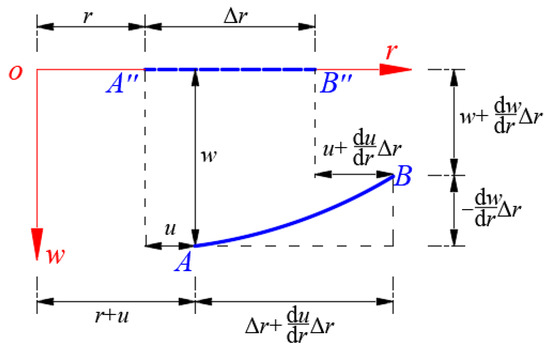
Figure 5. The geometric relationship between the micro radial straight line element $\overline{A^{″}{B}^{″}}$ and the micro meridional curve element $\stackrel{⌢}{AB}$.

The length of the straight line $\overline{A^{″}{B}^{″}}$ is $L_{\overline{A^{″}{B}^{″}}}=\Delta r$, while the length of the curve $\stackrel{⌢}{AB}$ may be approximated by

$$L_{\stackrel{⌢}{AB}}\approx L_{\overline{AB}}=\sqrt{(\Delta r+\frac{\mathrm{d}u}{\mathrm{d}r}\Delta r{)}^2+(-\frac{\mathrm{d}w}{\mathrm{d}r}\Delta r{)}^2}.$$

(13)

Therefore, for the radial deformation from the micro straight line element $\overline{A^{″}{B}^{″}}$ to the micro curve element $\stackrel{⌢}{AB}$, the line strain in the radial direction may be written as

$$e_r=\frac{L_{\stackrel{⌢}{AB}}-L_{\overline{A^{″}{B}^{″}}}}{L_{\overline{A^{″}{B}^{″}}}}=\frac{\sqrt{{(\Delta r+\frac{\mathrm{d}u}{\mathrm{d}r}\Delta r)}^2+(-\frac{\mathrm{d}w}{\mathrm{d}r}\Delta r{)}^2}-\Delta r}{\Delta r}=\sqrt{{(1+\frac{\mathrm{d}u}{\mathrm{d}r})}^2+{(-\frac{\mathrm{d}w}{\mathrm{d}r})}^2}-1.$$

(14)

On the other hand, if a micro curve element $\stackrel{⌢}{AD}$ along the circumferential direction on the deflected circular membrane is assumed to come from the deformation of a micro curve element $\stackrel{⌢}{A^{″}{D}^{″}}$ with radius r along the circumferential direction on the initially flat circular membrane located in the polar plane (r, φ), as shown in Figure 6, then the radial parallel distance between $\stackrel{⌢}{A^{″}{D}^{″}}$ and $\stackrel{⌢}{AD}$ should be equal to the radial displacement u.

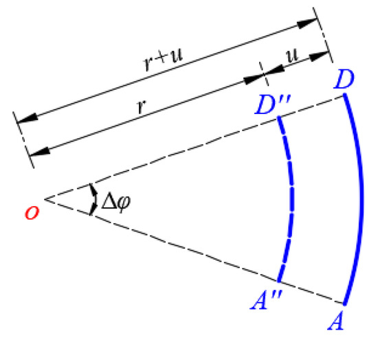
Figure 6. The geometric relationship between the circumferential curve micro elements $\stackrel{⌢}{A^{″}{D}^{″}}$ and $\stackrel{⌢}{AD}$.

Therefore, the lengths of the curves $\stackrel{⌢}{A^{″}{D}^{″}}$ and $\stackrel{⌢}{AD}$ are, respectively,

$$L_{\stackrel{⌢}{A^{″}{D}^{″}}}=r\cdot \Delta \phi$$

(15)

and

$$L_{\stackrel{⌢}{AD}}=(r+u)\cdot \Delta \phi .$$

(16)

Then, for the circumferential deformation from the micro curve element $\stackrel{⌢}{A^{″}{D}^{″}}$ to the micro curve element $\stackrel{⌢}{AD}$, the line strain in the circumferential direction may be written as

$$e_t=\frac{L_{\stackrel{⌢}{AD}}-L_{\stackrel{⌢}{A^{″}{D}^{″}}}}{L_{\stackrel{⌢}{A^{″}{D}^{″}}}}=\frac{(r+u)\cdot \Delta \phi -r\cdot \Delta \phi }{r\cdot \Delta \phi }=\frac{u}{r}.$$

(17)

Equations (14) and (17) are the so-called geometric equations for radial and circumferential deformations.

2.4. Formulation of Physical Equations

The relationships of stress and strain, i.e., the so-called physical equations, are assumed to satisfy generalized Hooke’s law, and are thus given by

$${\sigma }_r=\frac{E}{1-{\nu }^2}(e_r+\nu e_t)$$

(18)

and

$${\sigma }_t=\frac{E}{1-{\nu }^2}(e_t+\nu e_r).$$

(19)

2.5. Boundary Conditions

Equations (3), (12), (14), and (17)–(19) are six governing equations for solving stresses ${\sigma }_r$ and ${\sigma }_t$, strains $e_r$ and $e_t$, and displacements u and w. The boundary conditions for solving the above six governing equations are

$$\frac{\mathrm{d}w}{\mathrm{d}r}=0 \mathrm{at} r=0,$$

(20)

$$e_t=\frac{u}{r}=0 \mathrm{at} r=a$$

(21)

and

$$w=0 \mathrm{at} r=a.$$

(22)

2.6. Power Series Solutions to Governing Equations

Substituting Equations (14) and (17) into Equations (18) and (19), one has

$${\sigma }_r=\frac{E}{1-{\nu }^2}[\sqrt{(1+\frac{\mathrm{d}u}{\mathrm{d}r}{)}^2+(-\frac{\mathrm{d}w}{\mathrm{d}r}{)}^2}-1+\nu \frac{u}{r}]$$

(23)

and

$${\sigma }_t=\frac{E}{1-{\nu }^2}[\frac{u}{r}+\nu \sqrt{(1+\frac{\mathrm{d}u}{\mathrm{d}r}{)}^2+(-\frac{\mathrm{d}w}{\mathrm{d}r}{)}^2}-\nu ].$$

(24)

By means of Equations (23) and (24),

$$\frac{u}{r}=\frac{1}{E}({\sigma }_t-\nu {\sigma }_r).$$

(25)

Further, substituting the u in Equation (25) into Equation (23), the so-called consistency equation may be written as

$$(\frac{1}{E}{\sigma }_r-\frac{v}{E}{\sigma }_t+1{)}^2-[\frac{1}{E}\frac{\mathrm{d}(r{\sigma }_t)}{\mathrm{d}r}-\frac{v}{E}\frac{\mathrm{d}(r{\sigma }_r)}{\mathrm{d}r}+1{]}^2-(-\frac{\mathrm{d}w}{\mathrm{d}r}{)}^2=0.$$

(26)

Equations (3), (12), and (26) are three equations for the solutions of σ_r, σ_t, and w.

Let us introduce the following dimensionless variables

$$Q=\frac{aq}{hE},S_r=\frac{{\sigma }_r}{E},S_t=\frac{{\sigma }_t}{E},W=\frac{w}{a},U=\frac{u}{a},x=\frac{r}{a},$$

(27)

and transform Equations (3), (12), (25), and (26) into

$$(4S_r^2-x^2{Q}^2)(-\frac{\mathrm{d}W}{\mathrm{d}x}{)}^2-x^2{Q}^2=0,$$

(28)

$$\frac{\mathrm{d}(x{S}_r)}{\mathrm{d}x}[1+(-\frac{\mathrm{d}W}{\mathrm{d}x}{)}^2]-x{S}_r\frac{\mathrm{d}W}{\mathrm{d}x}\frac{{\mathrm{d}}^{2}W}{\mathrm{d}{x}^2}-S_t[1+(-\frac{\mathrm{d}W}{\mathrm{d}x}{)}^2{]}^2=0,$$

(29)

$$\frac{U}{x}=S_t-\nu S_r$$

(30)

and

$${(S_r-v{S}_t+1)}^2-[\frac{\mathrm{d}(x{S}_t)}{\mathrm{d}x}-v\frac{\mathrm{d}(x{S}_r)}{\mathrm{d}x}+1{]}^2-(-\frac{\mathrm{d}W}{\mathrm{d}x}{)}^2=0,$$

(31)

and transform the boundary condition Equations (20)–(22) into

$$\frac{\mathrm{d}W}{\mathrm{d}x}=0 \mathrm{at} x=0,$$

(32)

$$\frac{U}{x}=S_t-\nu S_r=0 \mathrm{at} x=1$$

(33)

and

$$W=0 \mathrm{at} x=1.$$

(34)

In general, in order to use the power series method to solve mathematical and physical differential equations, people may be accustomed to using the Maclaurin series (a power series in powers of x) rather than the Taylor series (a power series in powers of x − x₀) to expand physical variables such as stress, strain, and displacement. But in fact, the superiority of using Taylor series expansion over using Maclaurin series expansion has not yet been discovered, revealed, and well understood, including the relationship between the two. Therefore, we here use both Maclaurin series and Taylor series to expand S_r(x), S_t(x) and W(x), in order to show the difference between the two and which is better.

2.6.1. Power Series Solutions Using Maclaurin Series Expansion

In order to use the power series method to solve Equations (28), (29) and (31), we first use the Maclaurin series to expand S_r(x), S_t(x), and W(x), i.e., letting

$$S_r(x)={\displaystyle \sum _{i=0}^{\infty }{b}_i{x}^i},$$

(35)

$$S_t(x)={\displaystyle \sum _{i=0}^{\infty }{c}_i{x}^i}$$

(36)

and

$$W(x)={\displaystyle \sum _{i=0}^{\infty }{d}_i{x}^i}.$$

(37)

After substituting Equations (35)–(37) into Equations (28), (29) and (31) and, according to the same powers of the x, combining similar terms, all the sums of coefficients of the x with the same powers have to be equal to zero simultaneously to ensure that Equations (28), (29) and (31), after being substituted into Equations (35)–(37), hold regardless of the value taken by the x in the interval [0, 1]. This results in a system containing infinitely many equations with respect to the power series coefficients b_i, c_i, d_i. The recursion formulas for the power series coefficients b_i, c_i, d_i can be determined by solving this infinite system of equations, as shown in Appendix A, where b_i ≡ 0, c_i ≡ 0 and d_i ≡ 0 for i = 1, 3, 5, ⋯, and for i = 2, 4, 6, ⋯, the coefficients b_i, c_i, d_i can be expressed into the polynomial functions with regard to the coefficient b₀, while c₀ = b₀.

The coefficient b₀ is usually called an undetermined constant, while the remaining coefficient d₀ is another undetermined constant depending on the undetermined constant b₀. The undetermined constants b₀ and d₀ can be determined by using the boundary conditions Equations (33) and (34) as follows. From Equations (35)–(37), the conditions Equations (33) and (34) give

$${\displaystyle \sum _{i=0}^{\infty }{c}_i}-\nu {\displaystyle \sum _{i=0}^{\infty }{b}_i}=0$$

(38)

and

$$d_0=-{\displaystyle \sum _{i=1}^{\infty }{d}_i}.$$

(39)

Note that since all the coefficients b_i, c_i, d_i can be expressed as the polynomial functions with regard to only the coefficient b₀ (see Appendix A), Equation (38) contains only one variable b₀. Therefore, for a concrete problem in which the values of a, h, E, ν, and q are known beforehand, the undetermined constant b₀ can be determined by Equation (38), and the other coefficients b_i, c_i, d_i (i = 2, 4, 6, ⋯), and c₀ can be easily determined with the known b₀. Further, after substituting all the known d_i (i = 2, 4, 6, ⋯) into Equation (39), the remaining dependent undetermined constant d₀ can also be determined. Therefore, all the expressions of stresses σ_r and σ_t, strain e_r and e_t, and displacement u and w can finally be determined.

In addition, only two boundary conditions, i.e., Equations (33) and (34), are used to determine the undetermined constants b₀ and d₀ due to c₀ ≡ b₀, while the boundary condition Equation (32) has not been used yet. Now, let us examine whether the deflection solution W(x) satisfies the remaining boundary condition Equation (32), i.e., dW/dx = 0 at x = 0. Differentiating Equation (37) yields

$$\frac{\mathrm{dW}}{\mathrm{d}x}={\displaystyle \sum _{i=1}^{\infty }i{d}_i{x}^{i-1}}.$$

(40)

It can be found from Equation (40) that dW/dx = d₁ at x = 0. Therefore, since d₁ ≡ 0, then dW/dx ≡ 0 at x = 0, that is, the boundary condition Equation (32) can naturally be satisfied. This indicates that the power series solutions obtained by using power series in powers of x can satisfy all three boundary conditions Equations (32)–(34).

2.6.2. Power Series Solutions Using Taylor Series Expansion

Now we use the Taylor series expansion to solve Equations (28), (29), and (31). To this end, S_r(x), S_t(x), and W(x) have to be first expanded into the power series of the (x − x₀), where the series center x₀ should be placed in the middle of the interval [0, 1], i.e., x₀ takes 1/2; thus,

$$S_r(x)={\displaystyle \sum _{i=0}^{\infty }{b}_i(x-\frac{1}{2}{)}^i},$$

(41)

$$S_t(x)={\displaystyle \sum _{i=0}^{\infty }{c}_i(x-\frac{1}{2}{)}^i}$$

(42)

and

$$W(x)={\displaystyle \sum _{i=0}^{\infty }{d}_i(x-\frac{1}{2}{)}^i}.$$

(43)

For convenience, by introducing X = x − 1/2, Equations (41)–(43) are rewritten as

$$S_r(X)={\displaystyle \sum _{i=0}^{\infty }{b}_i{X}^i},$$

(44)

$$S_t(X)={\displaystyle \sum _{i=0}^{\infty }{c}_i{X}^i}$$

(45)

and

$$W(X)={\displaystyle \sum _{i=0}^{\infty }{d}_i{X}^i},$$

(46)

where X ∈ [−1/2, 1/2]. Also, Equations (28)–(34) need to be transformed into

$$[4S_r^2-(X+\frac{1}{2}{)}^2{Q}^2](-\frac{\mathrm{d}W}{\mathrm{d}X}{)}^2-(X+\frac{1}{2}{)}^2{Q}^2=0,$$

(47)

$$\frac{\mathrm{d}[(X+\frac{1}{2})S_r]}{\mathrm{d}X}[1+(-\frac{\mathrm{d}W}{\mathrm{d}X}{)}^2]-(X+\frac{1}{2})S_r\frac{\mathrm{d}W}{\mathrm{d}X}\frac{{\mathrm{d}}^{2}W}{\mathrm{d}{X}^2}-S_t[1+(-\frac{\mathrm{d}W}{\mathrm{d}X}{)}^2{]}^2=0,$$

(48)

$$\frac{U}{X+\frac{1}{2}}=S_t-\nu S_r,$$

(49)

$${(S_r-v{S}_t+1)}^2-[\frac{\mathrm{d}[(X+\frac{1}{2})S_t]}{\mathrm{d}X}-v\frac{\mathrm{d}[(X+\frac{1}{2})S_r]}{\mathrm{d}X}+1{]}^2-(-\frac{\mathrm{d}W}{\mathrm{d}X}{)}^2=0,$$

(50)

$$\frac{\mathrm{d}W}{\mathrm{d}X}=0 \mathrm{at} X=-\frac{1}{2},$$

(51)

$$\frac{U}{X+\frac{1}{2}}=S_t-\nu S_r=0 \mathrm{at} X=\frac{1}{2},$$

(52)

and

$$W=0 \mathrm{at} X=\frac{1}{2}.$$

(53)

After substituting Equations (44)–(46) into Equations (47), (48), and (50), and, according to the same powers of the x, combining similar terms, all the sums of coefficients of the x with the same powers have to be equal to zero simultaneously, to ensure that Equations (47), (48), and (50), after being substituted into Equations (44)–(46), hold regardless of the value taken by the X in the interval [−1/2, 1/2]. This results in a system containing infinitely many equations with respect to the power series coefficients b_i, c_i, d_i. The recursion formulas for the power series coefficients b_i, c_i, d_i can be determined by solving this infinite system of equations, as shown in Appendix B, where the coefficients b_i, c_i, d_i (i = 1, 2, 3, ⋯) can be expressed into the polynomial functions with regard to the coefficients b₀ and c₀. Therefore, for the case of using Taylor series expansion, there are two undetermined constants, i.e., the coefficients b₀ and c₀, while the remaining coefficient d₀ is also a dependent undetermined constant (it depends on the undetermined constants b₀ and c₀). This is clearly different from the case of using Maclaurin series expansion, where there is only one undetermined constant b₀ but two dependent undetermined constants c₀ and d₀, due to c₀ ≡ b₀ (see Appendix A).

The undetermined constants b₀, c₀, and d₀ can be determined by using the boundary condition Equations (51)–(53) as follows. From Equations (44)–(46), the boundary conditions Equations (51) and (52) give

$${\displaystyle \sum _{i=1}^{\infty }i{d}_i(-\frac{1}{2}{)}^{i-1}}=0$$

(54)

and

$${\displaystyle \sum _{i=0}^{\infty }{c}_i(\frac{1}{2}{)}^i}-\nu {\displaystyle \sum _{i=0}^{\infty }{b}_i(\frac{1}{2}{)}^i}=0.$$

(55)

Equations (54) and (55) are two equations containing only the undetermined constants b₀ and c₀, because the coefficients b_i, c_i, d_i (i = 1, 2, 3, ⋯) can be expressed into the polynomial functions with regard to the coefficients b₀ and c₀ (see Appendix B). Therefore, for a concrete problem in which the values of a, h, E, ν, and q are known beforehand, the undetermined constants b₀ and c₀ can be determined by simultaneously solving Equations (54) and (55). Then, the coefficients b_i, c_i, d_i (i = 1, 2, 3, ⋯) can be easily determined with the known b₀ and c₀. Furthermore, from Equation (46), the boundary condition Equation (53) gives

$$d_0=-{\displaystyle \sum _{i=1}^{\infty }{d}_i(\frac{1}{2}{)}^i}.$$

(56)

Therefore, after substituting the known d_i (i = 1,2,3,4, ⋯) into Equation (56), the remaining dependent undetermined constant d₀ can also be determined.

The expressions of S_r, S_t, and W can be finally determined, and the expressions of the dimensional quantities σ_r, σ_t, and w can also be determined. As for the expressions of e_r, e_t, and u, with the known expressions of σ_r, σ_t, and w, they can be easily derived by Equations (18), (19), and (25). Given the length of the article, their derivations are omitted here. In summary, the problem under consideration can, thus, be solved analytically.

3. Results and Discussions

Intuitively, if the center x₀ of the Taylor series takes zero, then the power series solutions using Taylor series expansion should become the power series solutions using Maclaurin series expansion. If this conjecture is true, then we can first use the Taylor series expansion to solve Equations (28), (29) and (31) without pre-specifying a concrete value of x₀, and then, easily let the x₀ in the obtained solutions be zero to obtain the solutions given in Section 2.6.1, and let the x₀ in the obtained solutions be 1/2 to obtain the solutions given in Section 2.6.2 easily. However, the conclusion from this study is that this conjecture is true only for the case where the x₀ takes any value within the interval (0, 1], but is not true for the case where the x₀ takes zero. In other words, the power series solutions using Taylor series expansion and using Maclaurin series expansion have nothing to do with each other. This is why we use Maclaurin series expansion (Section 2.6.1) and Taylor series expansion (Section 2.6.2) to solve Equations (28), (29) and (31) separately.

On the other hand, it can be seen from Section 2.6.1 and Section 2.6.2 that in the case of using Maclaurin series expansion (Section 2.6.1), there is only one undetermined constant b₀ and two dependent undetermined constants c₀ and d₀, while in the case of using Taylor series expansion (Section 2.6.2), there are two undetermined constants b₀ and c₀, and only one dependent undetermined constant d₀. This means that there is an essential difference between using Maclaurin series expansion and using Taylor series expansion.

In addition, the difference between using Maclaurin series expansion and using Taylor series expansion is also reflected in the convergence of the obtained power series solutions. It can be seen from the subsequent Section 3.1.1 and Section 3.1.2 that the use of Taylor series expansion has a clear convergence superiority over the use of Maclaurin series expansion.

It is worth mentioning that in the existing literature, there are no reports of research on the above-mentioned three issues.

3.1. Convergence Analysis

As can be seen from Appendix A and Appendix B, the recursion formulas of the power series coefficients b_i, c_i, d_i are quite complex. Therefore, in general, the convergence of power series solutions can only be analyzed numerically. To this end, a numerical example is considered; a circular membrane with radius a = 70 mm, thickness h = 0.3 mm, Young’s modulus of elasticity E = 3.01 MPa, and Poisson’s ratio ν = 0.45 is subjected to the uniformly distributed transverse loads q = 0.0001 MPa, 0.005 MPa, and 0.012 MPa, respectively.

The convergence analysis will begin with the numerical calculations of the undetermined constants b₀ and d₀ (the case of using Maclaurin series expansion) or b₀, c₀, and d₀ (the case of using Taylor series expansion). For the case of using Maclaurin series expansion, the undetermined constants b₀ and d₀ can be calculated by Equations (38) and (39), while for the case of using Taylor series expansion, the undetermined constants b₀, c₀, and d₀ can be calculated by Equations (54)–(56). Obviously, for convenience of practical calculation operation, all the infinite power series ${\displaystyle \sum _i^{\infty }}$ in Equations (38), (39) and (54)–(56) have to be replaced with the truncated form ${\displaystyle \sum _i^n}$, the nth partial sum of ${\displaystyle \sum _i^{\infty }}$. For the case of using Maclaurin series expansion, the numerical calculations of the undetermined constants b₀ and d₀ will begin with n = 2, as we shall see in Section 3.1.1, and for the case of using Taylor series expansion, the numerical calculations of the undetermined constants b₀, c₀, and d₀ will begin with n = 3, as we shall see in Section 3.1.2.

3.1.1. The Convergence When Using Maclaurin Series Expansion

The results of numerical calculations of the undetermined constants b₀ and d₀ are listed in Table 1, and the variations of the values of b₀ and d₀ with the parameter n are shown in Figure 7, Figure 8, Figure 9, Figure 10, Figure 11 and Figure 12. It can be seen from Figure 7, Figure 8, Figure 9, Figure 10, Figure 11 and Figure 12 that b₀ and d₀ converge only when q = 0.0001 MPa, and diverge both when q = 0.005 MPa and when q = 0.012 MPa.

Table 1. The results of numerical calculations of the undetermined constants b₀ and d₀.

n	q = 0.0001 MPa		q = 0.005 MPa		q = 0.012 MPa
	b0	d0	b0	d0	b0	d0
2	0.016169	0.119861	0.193170	0.501627	0.308604	0.753581
4	0.017197	0.121958	0.194231	0.481063	0.269089	0.657447
6	0.017409	0.121796	0.198052	0.485553	0.307288	0.735958
8	0.017466	0.121661	0.197643	0.481663	0.225534	0.215176
10	0.017483	0.121602	0.198348	0.483176	0.309685	0.806992
12	0.017489	0.121579	0.198152	0.481599	0.188651	0.477415
14	0.017491	0.121570	0.198342	0.482657	0.281565	2.375341
16	0.017491	0.121567	0.197866	0.481204	0.400863	0.807886
18	0.017491	0.121566	0.198838	0.483293	0.204223	3.829090
20	0.017491	0.121566	0.197574	0.483140	0.441707	0.929497

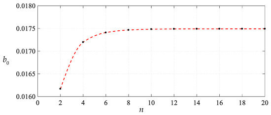
Figure 7. Variations of b₀ with n when q takes 0.0001 MPa.

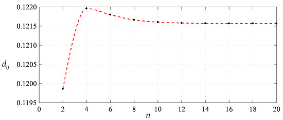
Figure 8. Variations of d₀ with n when q takes 0.0001 MPa.

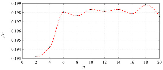
Figure 9. Variations of b₀ with n when q takes 0.005 MPa.

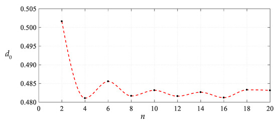
Figure 10. Variations of d₀ with n when q takes 0.005 MPa.

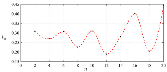
Figure 11. Variations of b₀ with n when q takes 0.012 MPa.

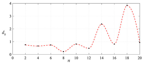
Figure 12. Variations of d₀ with n when q takes 0.012 MPa.

The power series coefficients b_i, c_i, and d_i when q = 0.0001 MPa are calculated using the values of b₀ and d₀ when q = 0.0001 MPa and n = 20 in Table 1, and the calculation results are listed in Table 2. The variations of the values of b_i, c_i, and d_i with the parameter i are shown in Figure 13, Figure 14 and Figure 15, from which the convergence of power series solutions at the end of the interval x ∈ [0, 1], i.e., at x = 1, can be observed; see Equations (35)–(37). It can be seen from Figure 13, Figure 14 and Figure 15 that b_i, c_i, and d_i converge when q = 0.0001 MPa. Obviously, when q = 0.005 MPa and 0.012 MPa, since the undetermined constants b₀ and d₀ diverge, the convergence of the coefficients b_i, c_i, and d_i is not necessary to be discussed.

Table 2. The calculation results of the power series coefficients b_i, c_i, and d_i when q = 0.0001 MPa.

i	bi	ci	di
0	0.017491	0.017491	0.121566
2	−2.299 × 10−3	−8.614 × 10−3	−1.108 × 10−1
4	−2.754 × 10−4	−1.603 × 10−3	−8.641 × 10−3
6	−5.116 × 10−5	−4.148 × 10−4	−1.610 × 10−3
8	−1.166 × 10−5	−1.210 × 10−4	−3.786 × 10−4
10	−2.985 × 10−6	−3.764 × 10−5	−1.002 × 10−4
12	−8.248 × 10−7	−1.222 × 10−5	−2.851 × 10−5
14	−2.405 × 10−7	−4.084 × 10−6	−8.523 × 10−6
16	−1.108 × 10−7	−1.277 × 10−6	−1.960 × 10−6
18	−3.655 × 10−8	−4.165 × 10−7	−5.770 × 10−7
20	−1.199 × 10−8	−1.392 × 10−7	−1.788 × 10−7

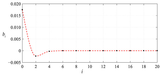
Figure 13. Variations of b_i with i when q takes 0.0001 MPa.

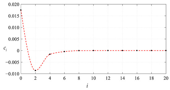
Figure 14. Variations of c_i with i when q takes 0.0001 MPa.

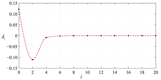
Figure 15. Variations of d_i with i when q takes 0.001 MPa.

Therefore, it can be concluded from Figure 7, Figure 8, Figure 9, Figure 10, Figure 11, Figure 12, Figure 13, Figure 14 and Figure 15 that in the interval x ∈ [0, 1], the power series solutions of radial stress S_r(x) and circumferential stress S_t(x) and transverse displacement W(x), which are derived by using Maclaurin series expansion, converge only when q = 0.0001 MPa, and diverge when q = 0.005 MPa and 0.012 MPa.

3.1.2. The Convergence When Using a Power Series in Powers of (x − 1/2)

The results of numerical calculation of the undetermined constants b₀, c₀, and d₀ are listed in Table 3, and the variations of the values of b₀, c₀, and d₀ with the parameter n are shown in Figure 16, Figure 17, Figure 18, Figure 19, Figure 20, Figure 21, Figure 22, Figure 23 and Figure 24. It can be seen from Figure 16, Figure 17, Figure 18, Figure 19, Figure 20, Figure 21, Figure 22, Figure 23 and Figure 24 that whether the uniformly distributed transverse loads q takes 0.0001 MPa, 0.005 MPa, or 0.012 MPa, the undetermined constants b₀, c₀, and d₀ always converge.

Table 3. The results of numerical calculation of the undetermined constants b₀, c₀, and d₀.

n	q = 0.0001 MPa			q = 0.005 MPa			q = 0.012 MPa
	b0	c0	d0	b0	c0	d0	b0	c0	d0
3	0.016292	0.013668	0.097291	0.221177	0.180552	0.363450	0.393014	0.290205	0.508047
4	0.016718	0.015038	0.094576	0.220879	0.182558	0.364409	0.390632	0.288871	0.515486
5	0.016828	0.015165	0.093735	0.222826	0.183804	0.361598	0.393688	0.291004	0.509066
6	0.016860	0.015200	0.093493	0.223041	0.184274	0.361110	0.393789	0.291508	0.510216
7	0.016888	0.015212	0.093368	0.223105	0.184385	0.360962	0.393968	0.291706	0.509820
8	0.016893	0.015226	0.093332	0.223154	0.184416	0.360908	0.394006	0.291809	0.509858
9	0.016897	0.015228	0.093312	0.223184	0.184445	0.360872	0.394056	0.291849	0.509829
10	0.016898	0.015230	0.093305	0.223189	0.184457	0.360859	0.394109	0.291876	0.509833
11	0.016898	0.015230	0.093305	0.223189	0.184457	0.360859	0.394109	0.291876	0.509833

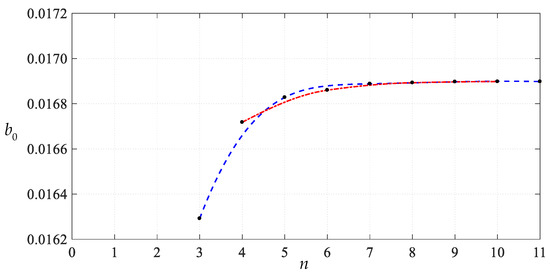
Figure 16. Variations of b₀ with n for q = 0.0001 MPa, where the blue dashed line corresponds to the case when n is odd and the red dotted line corresponds to the case when n is even.

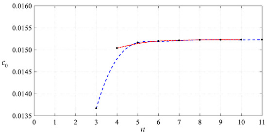
Figure 17. Variations of c₀ with n for q = 0.0001 MPa, where the blue dashed line corresponds to the case when n is odd and the red dotted line corresponds to the case when n is even.

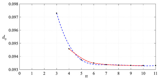
Figure 18. Variations of d₀ with n for q = 0.0001 MPa, where the blue dashed line corresponds to the case when n is odd and the red dotted line corresponds to the case when n is even.

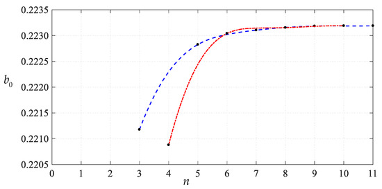
Figure 19. Variations of b₀ with n for q = 0.005 MPa, where the blue dashed line corresponds to the case when n is odd and the red dotted line corresponds to the case when n is even.

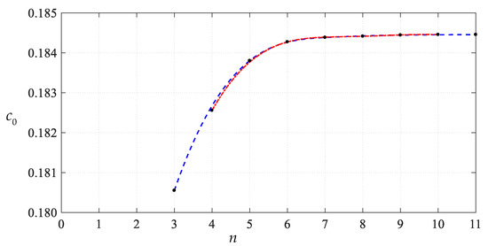
Figure 20. Variations of c₀ with n for q = 0.005 MPa, where the blue dashed line corresponds to the case when n is odd and the red dotted line corresponds to the case when n is even.

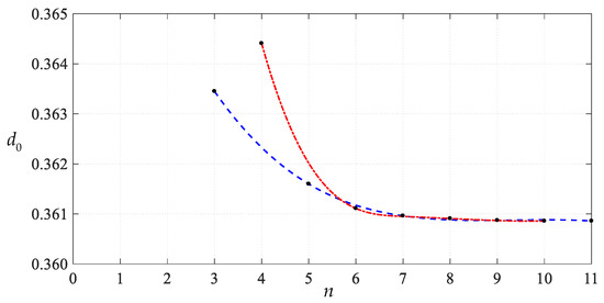
Figure 21. Variations of d₀ with n for q = 0.005 MPa, where the blue dashed line corresponds to the case when n is odd and the red dotted line corresponds to the case when n is even.

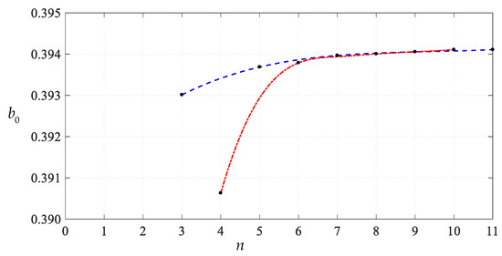
Figure 22. Variations of b₀ with n for q = 0.012 MPa, where the blue dashed line corresponds to the case when n is odd and the red dotted line corresponds to the case when n is even.

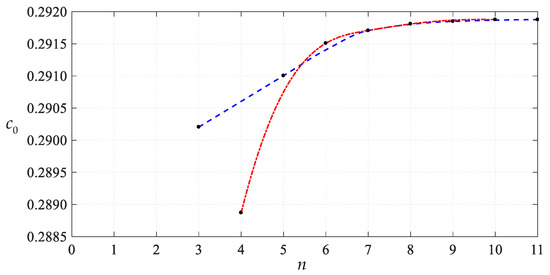
Figure 23. Variations of c₀ with n for q = 0.012 MPa, where the blue dashed line corresponds to the case when n is odd and the red dotted line corresponds to the case when n is even.

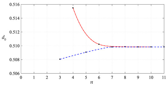
Figure 24. Variations of d₀ with n for q = 0.012 MPa, where the blue dashed line corresponds to the case when n is odd and the red dotted line corresponds to the case when n is even.

The values of b_i(x − 1/2)ⁱ, c_i(x − 1/2)ⁱ, and d_i(x − 1/2)ⁱ are calculated using the values of b₀, c₀, and d₀ when n = 11 in Table 3, and the calculation results are listed in Table 4 for q = 0.0001 MPa, in Table 5 for q = 0.005 MPa, and in Table 6 for q = 0.012 MPa. The variations of the values of b_i(x − 1/2)ⁱ, c_i(x − 1/2)ⁱ, and d_i(x − 1/2)ⁱ with the parameter i are shown in Figure 25, Figure 26, Figure 27, Figure 28, Figure 29, Figure 30, Figure 31, Figure 32 and Figure 33, from which the convergence of power series solutions at the two ends of the interval x ∈ [0, 1], i.e., at x = 0 and at x = 1, can be observed; see Equations (41)–(43). It can be seen from Figure 25, Figure 26, Figure 27, Figure 28, Figure 29, Figure 30, Figure 31, Figure 32 and Figure 33 that whether the uniformly distributed transverse loads q takes 0.0001 MPa, 0.005 MPa, or 0.012 MPa, b_i(x − 1/2)ⁱ, c_i(x − 1/2)ⁱ and d_i(x − 1/2)ⁱ always converge.

Table 4. The calculation results of b_i(x − 1/2)ⁱ, c_i(x − 1/2)ⁱ, and d_i(x − 1/2)ⁱ for q = 0.0001 MPa.

i	x = 1			x = 0
	bi(x − 1/2)i	ci(x − 1/2)i	di(x − 1/2)i	bi(x − 1/2)i	ci(x − 1/2)i	di(x − 1/2)i
0	1.689 × 10−2	1.523 × 10−2	9.331 × 10−2	1.690 × 10−2	1.523 × 10−2	9.331 × 10−2
1	−1.223 × 10−3	−4.752 × 10−3	−5.773 × 10−2	1.223 × 10−3	4.752 × 10−3	5.773 × 10−2
2	−6.919 × 10−4	−2.867 × 10−3	−3.137 × 10−2	−6.919 × 10−4	−2.867 × 10−3	−3.137 × 10−2
3	−8.723 × 10−5	−5.628 × 10−4	−2.761 × 10−3	8.723 × 10−5	5.628 × 10−4	2.761 × 10−3
4	−3.387 × 10−5	−2.393 × 10−4	−1.046 × 10−3	−3.387 × 10−5	−2.393 × 10−4	−1.046 × 10−3
5	−7.384 × 10−6	−7.853 × 10−5	−2.654 × 10−4	7.384 × 10−6	7.853 × 10−5	2.654 × 10−4
6	−3.976 × 10−6	−3.010 × 10−5	−9.547 × 10−5	−3.976 × 10−6	−3.010 × 10−5	−9.547 × 10−5
7	2.587 × 10−6	−1.295 × 10−5	−3.154 × 10−5	−2.587 × 10−6	1.295 × 10−5	3.154 × 10−5
8	−1.691 × 10−6	−3.372 × 10−6	−1.154 × 10−5	−1.691 × 10−6	−3.372 × 10−6	−1.154 × 10−5
9	1.381 × 10−6	−3.009 × 10−6	−4.282 × 10−6	−1.381 × 10−6	3.009 × 10−6	4.282 × 10−6
10	−1.700 × 10−7	−8.860 × 10−7	−1.561 × 10−6	−1.700 × 10−7	−8.860 × 10−7	−1.561 × 10−6
11	1.665 × 10−7	−2.589 × 10−7	−2.081 × 10−7	−1.665 × 10−7	2.589 × 10−7	2.081 × 10−7

Table 5. The calculation results of b_i(x − 1/2)ⁱ, c_i(x − 1/2)ⁱ and d_i(x − 1/2)ⁱ for q = 0.005 MPa.

i	x = 1			x = 0
	bi(x − 1/2)i	ci(x − 1/2)i	di(x − 1/2)i	bi(x − 1/2)i	ci(x − 1/2)i	di(x − 1/2)i
0	2.232 × 10−1	1.845 × 10−1	3.609 × 10−1	2.232 × 10−1	1.845 × 10−1	3.609 × 10−1
1	4.541 × 10−2	−3.027 × 10−2	−2.410 × 10−1	−4.541 × 10−2	3.027 × 10−2	2.410 × 10−1
2	1.104 × 10−2	−2.028 × 10−2	−1.183 × 10−1	1.104 × 10−2	−2.028 × 10−2	−1.183 × 10−1
3	−2.893 × 10−3	−5.376 × 10−3	−1.091 × 10−3	2.893 × 10−3	5.376 × 10−3	1.091 × 10−3
4	1.311 × 10−3	−1.933 × 10−3	−8.065 × 10−4	1.311 × 10−3	−1.933 × 10−3	−8.065 × 10−4
5	3.467 × 10−4	−7.753 × 10−4	4.744 × 10−4	−3.467 × 10−4	7.753 × 10−4	−4.744 × 10−4
6	−2.506 × 10−4	−4.330 × 10−4	−1.080 × 10−4	−2.506 × 10−4	−4.330 × 10−4	−1.080 × 10−4
7	1.717 × 10−5	−1.659 × 10−4	−4.369 × 10−5	−1.717 × 10−5	1.659 × 10−4	4.369 × 10−5
8	7.958 × 10−6	−6.467 × 10−5	−3.273 × 10−5	7.958 × 10−6	−6.467 × 10−5	−3.273 × 10−5
9	−3.384 × 10−6	−5.945 × 10−5	−7.449 × 10−6	3.384 × 10−6	5.945 × 10−5	7.449 × 10−6
10	−1.387 × 10−6	−6.117 × 10−6	−2.716 × 10−6	−1.387 × 10−6	−6.117 × 10−6	−2.716 × 10−6
11	1.661 × 10−7	−2.572 × 10−6	−2.065 × 10−7	−1.661 × 10−7	2.572 × 10−6	2.065 × 10−7

Table 6. The calculation results of b_i(x − 1/2)ⁱ, c_i(x − 1/2)ⁱ, and d_i(x − 1/2)ⁱ for q = 0.012 MPa.

i	x = 1			x = 0
	bi(x − 1/2)i	ci(x − 1/2)i	di(x − 1/2)i	bi(x − 1/2)i	ci(x − 1/2)i	di(x − 1/2)i
0	3.941 × 10−1	2.919 × 10−1	5.098 × 10−1	3.941 × 10−1	2.919 × 10−1	5.098 × 10−1
1	1.722 × 10−1	−7.288 × 10−3	−3.655 × 10−1	−1.722 × 10−1	7.288 × 10−3	3.655 × 10−1
2	3.862 × 10−2	−6.277 × 10−3	−1.578 × 10−1	3.862 × 10−2	−6.277 × 10−3	−1.578 × 10−1
3	−2.335 × 10−2	−4.856 × 10−3	1.683 × 10−2	2.335 × 10−2	4.856 × 10−3	−1.683 × 10−2
4	9.121 × 10−3	−1.172 × 10−3	−2.661 × 10−3	9.121 × 10−3	−1.172 × 10−3	−2.661 × 10−3
5	−1.704 × 10−3	−1.037 × 10−3	−1.188 × 10−3	1.704 × 10−3	1.037 × 10−3	1.188 × 10−3
6	−1.198 × 10−3	−9.729 × 10−5	7.394 × 10−4	−1.198 × 10−3	−9.729 × 10−5	7.394 × 10−4
7	1.101 × 10−3	−8.095 × 10−4	−2.746 × 10−4	−1.101 × 10−3	8.095 × 10−4	2.746 × 10−4
8	−7.617 × 10−4	−7.503 × 10−4	−6.031 × 10−5	−7.617 × 10−4	−7.503 × 10−4	−6.031 × 10−5
9	1.625 × 10−4	−5.544 × 10−5	5.748 × 10−5	−1.625 × 10−4	5.544 × 10−5	−5.748 × 10−5
10	1.145 × 10−4	−5.256 × 10−5	−3.611 × 10−5	1.145 × 10−4	−5.256 × 10−5	−3.611 × 10−5
11	−1.418 × 10−5	−1.010 × 10−5	8.009 × 10−6	1.418 × 10−5	1.010 × 10−5	−8.009 × 10−6

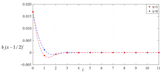
Figure 25. Variations of b_i(x − 1/2)ⁱ with i for q = 0.0001 MPa, where the dashed line with squares corresponds to the case when x = 1 and the dashed line with triangles corresponds to the case when x = 0.

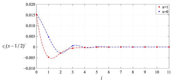
Figure 26. Variations of c_i(x − 1/2)ⁱ with i for q = 0.0001 MPa, where the dashed line with squares corresponds to the case when x = 1 and the dashed line with triangles corresponds to the case when x = 0.

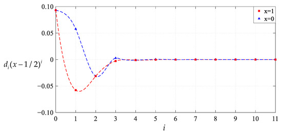
Figure 27. Variations of d_i(x − 1/2)ⁱ with i for q = 0.0001 MPa, where the dashed line with squares corresponds to the case when x = 1 and the dashed line with triangles corresponds to the case when x = 0.

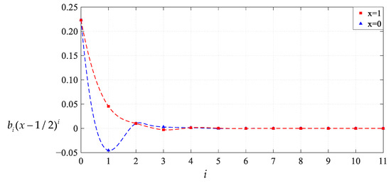
Figure 28. Variations of b_i(x − 1/2)ⁱ with i for q = 0.005 MPa, where the dashed line with squares corresponds to the case when x = 1 and the dashed line with triangles corresponds to the case when x = 0.

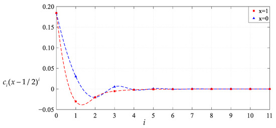
Figure 29. Variations of c_i(x − 1/2)ⁱ with i for q = 0.005 MPa, where the dashed line with squares corresponds to the case when x = 1 and the dashed line with triangles corresponds to the case when x = 0.

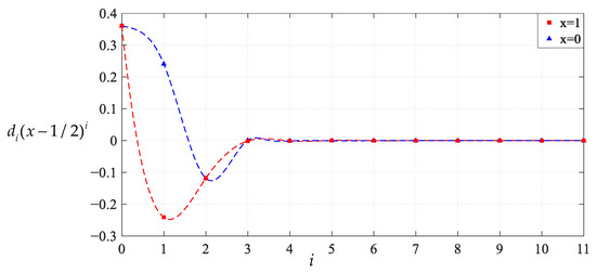
Figure 30. Variations of d_i(x − 1/2)ⁱ with i for q = 0.005 MPa, where the dashed line with squares corresponds to the case when x = 1 and the dashed line with triangles corresponds to the case when x = 0.

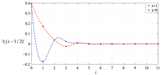
Figure 31. Variations of b_i(x − 1/2)ⁱ with i for q = 0.012 MPa, where the dashed line with squares corresponds to the case when x = 1 and the dashed line with triangles corresponds to the case when x = 0.

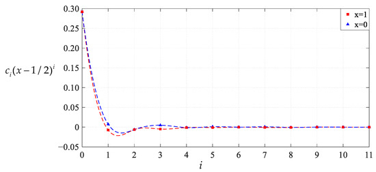
Figure 32. Variations of c_i(x − 1/2)ⁱ with i for q = 0.012 MPa, where the dashed line with squares corresponds to the case when x = 1 and the dashed line with triangles corresponds to the case when x = 0.

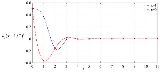
Figure 33. Variations of d_i(x − 1/2)ⁱ with i for q = 0.012 MPa, where the dashed line with squares corresponds to the case when x = 1 and the dashed line with triangles corresponds to the case when x = 0.

Therefore, it can be concluded from Figure 16, Figure 17, Figure 18, Figure 19, Figure 20, Figure 21, Figure 22, Figure 23, Figure 24, Figure 25, Figure 26, Figure 27, Figure 28, Figure 29, Figure 30, Figure 31, Figure 32 and Figure 33 that whether the uniformly distributed transverse loads q takes 0.0001 MPa, 0.005 MPa, or 0.012 MPa, the power series solutions of radial stress S_r(x) and circumferential stress S_t(x) and transverse displacement W(x), which are derived by using power series in powers of (x − 1/2), always converge in the interval x ∈ [0, 1].

3.2. The Superiority of the New In-Plane Equilibrium Equation over the Existing Two

Up to this study, three versions of the in-plane equilibrium equations have been used to analytically solve the well-known Föppl-Hencky membrane problem; they are the classical Föppl-von Kármán version used originally by Hencky [25]

$$\frac{\mathrm{d}}{\mathrm{d}r}(r{\sigma }_r)-{\sigma }_t=0,$$

(57)

the previously improved version presented originally by Li et al. [45]

$$\frac{\mathrm{d}}{\mathrm{d}r}(r{\sigma }_r)-{\sigma }_t\sqrt{1+{(-\mathrm{d}w/\mathrm{d}r)}^2}=0,$$

(58)

and the current improved version in this paper, Equation (12) (re-listed here for the convenience of comparison),

$$\frac{\mathrm{d}}{\mathrm{d}r}(\frac{r{\sigma }_r}{\sqrt{1+{(-\mathrm{d}w/\mathrm{d}r)}^2}})-{\sigma }_t\sqrt{1+{(-\mathrm{d}w/\mathrm{d}r)}^2}=0.$$

(59)

It can be seen from the comparison between Equations (57)–(59) that if the membrane rotation angle θ is always equal to zero during the deflection of the circular membrane, then tanθ = −dw/dr ≡ 0, such that Equations (59) and (58) can be reduced to Equation (57). Therefore, the classical in-plane equilibrium equation, Equation (57), actually ignores the contribution of the transverse displacement w to in-plane equilibrium, and more precisely, it only applies to the in-plane stretching problem, rather than the deflection problem of membranes.

On the other hand, however, it can also be seen from the comparison between Equations (57)–(59) that Equation (57) can be obtained by letting dw/dr in Equations (59) and (58) be zero, but Equation (58) cannot be obtained by letting dw/dr in Equation (59) be zero. This problem arises from the use of the inappropriate assumption in the reference [45]. The use of the assumption between Equations (A4) and (A5) in the reference [45] is incorrect (the condition of Δrγ0 can only be used to take limits to equations), resulting in an incorrect equation, i.e., Equation (A5) in the reference [45]. Therefore, Equation (58) is, strictly speaking, an incorrect in-plane equilibrium equation, but it is often regarded not as an incorrect equation, but as an approximate in-plane equilibrium equation that may cause errors.

Now let us examine how many approximate errors can be caused by Equations (57) and (58). To this end, the numerical example used in Section 3.2 is still used here. The same out-of-plane equilibrium equation, geometric equations, and physical equations as Equation (3), Equations (14) and (17), and Equations (18) and (19) in this paper are used in the references [22,46], and the above three in-plane equilibrium equations, Equations (57)–(59), are used in the reference [22], in the reference [46] and in this paper, respectively. Therefore, in order to make a comparison under the same conditions, the power series solutions presented in the references [22,46] are used for comparison here. The difference between the power series solutions presented in the reference [22], in the reference [46] and in this paper depends only on the difference between the above three in-plane equilibrium equations, i.e., Equations (57)–(59).

Figure 34 shows the variations of the deflection w with the radial coordinate r and uniformly distributed transverse loads q, where the “Solution 1” refers to the results calculated by using the power series solution presented in this paper, “Solution 2” refers to the results calculated by using the power series solution presented in the reference [46], and “Solution 3” refers to the results calculated by using the power series solution presented in the reference [22].

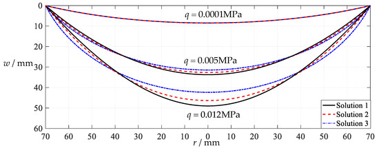
Figure 34. Variations of w with r when q takes 0.0001 MPa, 0.005 MPa, and 0.012 MPa.

It can be seen from Figure 34 that the relative errors of Solutions 3 and 2 to Solution 1 increase with the increase of the loads q, and the relative error of Solution 3 to Solution 1 is always greater than that of Solution 2 to Solution 1. Therefore, the new in-plane equilibrium equation, Equation (59), does perform much better than the classical version Equation (57) and previously improved version Equation (58), especially for heavily loaded membranes. On the other hand, although the previously improved in-plane equilibrium equation, Equation (58), is incorrect, it does partly take into account the contribution of deflection to in-plane equilibrium, in comparison with the classical version Equation (57). However, the approximate errors brought by using Equation (58) are also substantial, especially for heavily loaded membranes. Thus, the previously improved in-plane equilibrium equation, Equation (58), should be abandoned and replaced by the new in-plane equilibrium equation, Equation (59).

4. Concluding Remarks

In this paper, the well-known Hencky problem is reformulated and is analytically solved. From this study, the following conclusions can be drawn.

The classical in-plane equilibrium equation, Equation (57), does not take into account the contribution of deflection to in-plane equilibrium, so it is only applicable to the problem of the in-plane tension or compression of membranes or thin plates, rather than the large deflection problem of transversely loaded membranes or thin plates. The previously presented in-plane equilibrium equation, Equation (58), only takes into account the partial contribution of deflection to in-plane equilibrium, and thus, may induce substantial approximate errors if used for large deflection membranes. The new in-plane equilibrium equation presented here, Equation (59) or (12), takes into account the full contribution of deflection to in-plane equilibrium, and thus, can be used for the large deflection problem of transversely loaded membranes or thin plates.

The power series method of using the Taylor series expansion (i.e., using a power series in powers of x − x₀) differs from that of using the Maclaurin series expansion (i.e., using a power series in powers of x) in that, since the center x₀ of the used Maclaurin series is at the left endpoint of the domain [0, 1] of the independent variables x (i.e., at x₀ = 0), the radius of convergence necessary for the used Maclaurin series to satisfy the boundary conditions at the right endpoint of the domain [0, 1], i.e., to satisfy Equations (33) and (34), is 1, while if the center x₀ of the used Taylor series is placed in the middle of the domain [0, 1] of the independent variables x (i.e., x₀ takes 1/2), then the radius of convergence necessary for the used Taylor series to satisfy Equations (33) and (34) is 1/2. Therefore, the use of the Taylor series expansion is beneficial to the improvement of convergence, in comparison with the use of the Maclaurin series expansion.

However, the resulting recurrence relations or recursion formulas of power series coefficients obtained by using the Taylor series expansion, it should be noted, are different from those obtained by using the Maclaurin series expansion. In other words, the coefficient recurrence formulas of using the Maclaurin series expansion cannot be directly obtained by simply setting the series center x₀ in the coefficient recursion formulas of using the Taylor series expansion to zero.

References

- Goloskokov, D.P.; Matrosov, A.V. Bending of clamped orthotropic thin plates: Polynomial solution. Math. Mech. Solids 2022, 27, 2498–2509. [Google Scholar] [CrossRef]
- Gharahi, A.; Schiavone, P. On the boundary value problems of bending of thin elastic plates with surface effects. ASME J. Appl. Mech. 2021, 88, 021007. [Google Scholar] [CrossRef]
- He, X.-T.; Ai, J.-C.; Li, Z.-Y.; Peng, D.-D.; Sun, J.-Y. Nonlinear large deformation problem of rectangular thin plates and its perturbation solution under cylindrical bending: Transform from plate/membrane to beam/cable. Z. Angew. Math. Mech. 2022, 102, e202100306. [Google Scholar] [CrossRef]
- Liu, C.S.; Qiu, L.; Lin, J. Simulating thin plate bending problems by a family of two-parameter homogenization functions. Appl. Math. Model. 2020, 79, 284–299. [Google Scholar]
- Zenkour, A.M. Bending of thin rectangular plates with variable-thickness in a hygrothermal environment. Thin-Walled Struct. 2018, 123, 333–340. [Google Scholar] [CrossRef]
- Sun, J.-Y.; Zhang, Q.; Wu, J.; Li, X.; He, X.-T. Large Deflection Analysis of Peripherally Fixed Circular Membranes Subjected to Liquid Weight Loading: A Refined Design Theory of Membrane Deflection-Based Rain Gauges. Materials 2021, 14, 5992. [Google Scholar] [CrossRef] [PubMed]
- Sun, J.-Y.; Hu, J.-L.; He, X.-T.; Zheng, Z.-L.; Geng, H.-H. A Theoretical Study of Thin Film Delamination Using Clamped Punch-Loaded Blister Test: Energy Release Rate and Closed-Form Solution. J. Adhes. Sci. Technol. 2011, 25, 2063–2080. [Google Scholar]
- Ma, Y.; Wang, G.R.; Chen, Y.L.; Long, D.; Guan, Y.C.; Liu, L.Q.; Zhang, Z. Extended Hencky solution for the blister test of nanomembrane. Extrem. Mech. Lett. 2018, 22, 69–78. [Google Scholar] [CrossRef]
- Feng, L.; Li, X.; Shi, T. Nonlinear large deflection of thin film overhung on compliant substrate using shaft-loaded blister test. J. Appl. Mech. 2015, 82, 091001. [Google Scholar] [CrossRef]
- Zhang, C.H.; Fan, L.J.; Tan, Y.F. Sequential limit analysis for clamped circular membranes involving large deformation subjected to pressure load. Int. J. Mech. Sci. 2019, 155, 440–449. [Google Scholar] [CrossRef]
- Maurin, B.; Motro, R. Concrete shells form-finding with surface stress density method. J. Struct. Eng.-ASCE 2004, 130, 961–968. [Google Scholar] [CrossRef]
- Belles, P.; Ortega, N.; Rosales, M.; Andres, O. Shell form-finding: Physical and numerical design tools. Eng. Struct. 2009, 31, 2656–2666. [Google Scholar] [CrossRef]
- Aish, F.; Joyce, S.; Malek, S.; Williams, C.J.K. The use of a particle method for the modelling of isotropic membrane stress for the form finding of shell structures. Comput. Aided Des. 2015, 61, 24–31. [Google Scholar] [CrossRef]
- Chiang, Y.C.; Borgart, A. A form-finding method for membrane shells with radial basis functions. Eng. Struct. 2022, 251, 113514. [Google Scholar] [CrossRef]
- Sun, J.-Y.; Zhang, Q.; Li, X.; He, X.-T. Axisymmetric large deflection elastic analysis of hollow annular membranes under transverse uniform loading. Symmetry 2021, 13, 1770. [Google Scholar] [CrossRef]
- Zhang, Q.; Li, X.; He, X.-T.; Sun, J.-Y. Revisiting the boundary value problem for uniformly transversely loaded hollow annular membrane structures: Improvement of the out-of-plane equilibrium equation. Mathematics 2020, 10, 1305. [Google Scholar] [CrossRef]
- Sun, J.-Y.; Qian, S.-H.; Li, Y.-M.; He, X.-T.; Zheng, Z.-L. Theoretical study of adhesion energy measurement for film/substrate interface using pressurized blister test: Energy release rate. Measurement 2013, 46, 2278–2287. [Google Scholar] [CrossRef]
- Lim, T.C. Large deflection of circular auxetic membranes under uniform load. ASME J. Appl. Mech. 2016, 138, 041011. [Google Scholar] [CrossRef]
- Lian, Y.-S.; Sun, J.-Y.; Ge, X.-M.; Yang, Z.-X.; He, X.-T.; Zheng, Z.L. A theoretical study of an improved capacitive pressure sensor: Closed-form solution of uniformly loaded annular membranes. Measurement 2017, 111, 84–92. [Google Scholar] [CrossRef]
- Huang, P.F.; Song, Y.P.; Li, Q.; Liu, X.Q.; Feng, Y.Q. A theoretical study of circular orthotropic membrane under concentrated load: The relation of load and deflection. IEEE Access 2020, 8, 126127–126137. [Google Scholar]
- Yuan, J.H.; Liu, X.L.; Xia, H.B.; Huang, Y. Analytical solutions for inflation of pre-stretched elastomeric circular membranes under uniform pressure. Theor. Appl. Mech. Lett. 2021, 3, 130–136. [Google Scholar] [CrossRef]
- Lian, Y.S.; Sun, J.Y.; Zhao, Z.H.; He, X.T.; Zheng, Z.L. A revisit of the boundary value problem for Föppl–Hencky membranes: Improvement of geometric equations. Mathematics 2020, 8, 631. [Google Scholar] [CrossRef]
- Föppl, A. Vorlesungen über technische Mechanik: Bd. Die wichtigsten Lehren der höheren Elastizitätstheorie. BG Teubnerv. 1907, 5, 132–144. [Google Scholar]
- von Kármán, T. Festigkeitsprobleme im maschinenbau. Encykl. Math. Wiss. 1910, IV4, 349. [Google Scholar]
- Hencky, H. On the stress state in circular plates with vanishing bending stiffness. Z. Angew. Math. Phys. 1915, 63, 311–317. (In German) [Google Scholar]
- Chien, W.Z. Asymptotic behavior of a thin clamped circular plate under uniform normal pressure at very large deflection. Sci. Rep. Natl. Tsinghua Univ. 1948, 5, 193–208. (In Chinese) [Google Scholar]
- Alekseev, S.A. Elastic circular membranes under the uniformly distributed loads. Eng. Corpus 1953, 14, 196–198. (In Russian) [Google Scholar]
- Sun, J.Y.; Rong, Y.; He, X.T.; Gao, X.W.; Zheng, Z.L. Power series solution of circular membrane under uniformly distributed loads: Investigation into Hencky transformation. Stuct. Eng. Mech. 2013, 45, 631–641. [Google Scholar] [CrossRef]
- Lian, Y.S.; Sun, J.Y.; Yang, Z.X.; He, X.T.; Zheng, Z.L. Closed-form solution of well-known Hencky problem without small-rotation-angle assumption. Z. Angew. Math. Mech. 2016, 96, 1434–1441. [Google Scholar] [CrossRef]
- Way, S. Bending of circular plates with large deflection. ASME J. Appl. Mech. 1934, 56, 627–636. [Google Scholar] [CrossRef]
- Chien, W.Z. Large deflection of a circular clamped plate under uniform pressure. Chin. J. Phys. 1947, 7, 102–113. [Google Scholar]
- Chien, W.Z.; Chen, S.L. The solution of large deflection problem of thin circular plate by the method of composite expansion. Appl. Math. Mech. 1985, 6, 25–49. (In Chinese) [Google Scholar]
- Sheploak, M.; Dugundji, J. Large deflections of clamped circular plates under initial tension and transitions to membrane behavior. ASME J. Appl. Mech. 1998, 65, 107–111. [Google Scholar] [CrossRef]
- He, J.H. A Lagrangian for von Karman equations of large deflection problem of thin circular plate. Appl. Math. Comput. 2003, 143, 543–549. [Google Scholar] [CrossRef]
- Chen, Y.Z. Innovative iteration technique for nonlinear ordinary differential equations of large deflection problem of circular plates. Mech. Res. Commun. 2012, 43, 75–79. [Google Scholar] [CrossRef]
- Razdolsky, A.G. Determination of Large Deflections for Elastic Circular Plate. Proc. Inst. Civil Eng.-Eng. Comput. Mech. 2018, 171, 23–28. [Google Scholar] [CrossRef]
- Liu, X.J.; Zhou, Y.H.; Wang, J.Z. Highly Accurate Wavelet Solution for Bending and Free Vibration of Circular Plates over Extra-Wide Ranges of Deflections. ASME J. Appl. Mech. 2023, 90, 31009. [Google Scholar] [CrossRef]
- Kelkar, A.; Elber, W.; Raju, I.S. Large deflections of circular isotropic membranes subjected to arbitrary axisymmetric loading. Comput. Struct. 1985, 21, 413–421. [Google Scholar] [CrossRef]
- Komaragiri, U.; Begley, M.R.; Simmonds, J.G. The mechanical response of freestanding circular elastic films under point and pressure loads. ASME J. Appl. Mech. 2005, 72, 203–212. [Google Scholar] [CrossRef]
- Jin, C.R. Large deflection of circular membrane under concentrated force. Appl. Math. Mech. 2008, 29, 889–896. [Google Scholar] [CrossRef]
- Jin, C.; Wang, X.D. A theoretical study of a thin-film delamination using shaft-loaded blister test: Constitutive relation without delamination. J. Mech. Phys. Solids 2008, 56, 2815–2831. [Google Scholar] [CrossRef]
- Jin, C.R. Theoretical study of mechanical behavior of thin circular film adhered to a flat punch. Int. J. Mech. Sci. 2009, 51, 481–489. [Google Scholar] [CrossRef]
- Plaut, R.H. Linearly elastic annular and circular membranes under radial, transverse, and torsional loading. Part I: Large unwrinkled axisymmetric deformations. Acta Mech. 2009, 202, 79–99. [Google Scholar] [CrossRef]
- Zhang, Y.D.; Shui, L.Q.; Liu, Y.S. Deflection of film under biaxial tension and central concentrated load. Arch. Appl. Mech. 2022, 92, 2637–2646. [Google Scholar] [CrossRef]
- Li, X.; Sun, J.Y.; Zhao, Z.H.; Li, S.Z.; He, X.T. A new solution to well-known Hencky problem: Improvement of in-plane equilibrium equation. Mathematics 2020, 8, 653. [Google Scholar] [CrossRef]
- Lian, Y.S.; Sun, J.Y.; Zhao, Z.H.; Li, S.Z.; Zheng, Z.L. A refined theory for characterizing adhesion of elastic coatings on rigid substrates based on pressurized blister test methods: Closed-form solution and energy release rate. Polymers 2020, 12, 1788. [Google Scholar] [CrossRef] [PubMed]
Disclaimer/Publisher’s Note: The statements, opinions and data contained in all publications are solely those of the individual author(s) and contributor(s) and not of MDPI and/or the editor(s). MDPI and/or the editor(s) disclaim responsibility for any injury to people or property resulting from any ideas, methods, instructions or products referred to in the content. |
© 2023 by the authors. Licensee MDPI, Basel, Switzerland. This article is an open access article distributed under the terms and conditions of the Creative Commons Attribution (CC BY) license (https://creativecommons.org/licenses/by/4.0/).