A Symbolic Approach to Discrete Structural Optimization Using Quantum Annealing

Abstract

With the advent of novel quantum computing technologies and the new possibilities thereby offered, a prime opportunity has presented itself to investigate the practical application of quantum computing. This work investigates the feasibility of using quantum annealing for structural optimization. The target problem is the discrete truss sizing problem—the goal is to select the best size for each truss member so as to minimize a stress-based objective function. To make the problem compatible with quantum annealing devices, the objective function must be translated into a quadratic unconstrained binary optimization (QUBO) form. This work focuses on exploring the feasibility of making this translation. The practicality of using a quantum annealer for such optimization problems is also assessed. A method is eventually established to translate the objective function into a QUBO form and have it solved by a quantum annealer. However, scaling the method to larger problems faces some challenges that would require further research to address.

1. Introduction

Quantum computers are rather unique devices which leverage quantum mechanical principles to solve certain types of problems much more efficiently than classical computers [1]. While classical computers use binary bits, 1’s and 0’s, to perform their computations, quantum computers make use of quantum bits. Quantum bits, or qubits, can represent not only the classical 0 and 1 states, but also the quantum superposition of these states. This quantum superposition, when leveraged effectively, is one of the reasons why quantum computers promise better performance in certain applications.

There are two main types of quantum computers currently in development, namely, the general-purpose quantum computer (GPQC) and the quantum annealer (QA). With the GPQC, most of the potential improvements stem from the fact that these systems can run complex algorithms using quantum gates, allowing for more efficient problem-solving methods to be devised. An overview of quantum algorithms is given by Montanaro [2]. On the other hand, a QA can only use the quantum annealing algorithm, which is an optimization algorithm inspired by simulated annealing and quantum tunneling effects [3,4]. It is based on the adiabatic theorem, where a time-dependent Hamiltonian is constructed to gradually evolve the system from an initial, easily prepared Hamiltonian to the final, problem-specific Hamiltonian. Quantum tunneling will allow the system to stay in the ground state of the instantaneous Hamiltonian if the evolution is slow enough [5,6,7]. The quantum annealing algorithm solves very specific types of optimization problems, known as quadratic unconstrained binary optimization (QUBO) or Ising model problems [8].

Both quantum computing technologies are still in their infancy as compared to the advanced state of classical computing technologies. However, some recent studies on quantum(-inspired) computing applications have already shown promising results [9,10,11,12,13,14,15,16]. A review of their application in structural mechanics is given by Tosti Balducci et al. [17]. Furthermore, in the industry, some companies are already pushing for the development of early practical applications of quantum computing [18,19]. For example, Airbus posted the Airbus Quantum Computing Challenge, where one of the problems was to optimize a wingbox structure, the main load-bearing component in aircraft wings, using a quantum computer [20]. Another example comes from Volkswagen, which investigated how a QA could be used to optimize the traffic flow [10]. Volkswagen has already applied this research for the real-time optimization of public transport routes in Lisbon [21].

In the aerospace industry, there is a continuous demand to develop the lightest structures possible, so as to increase fuel efficiency/payload capacity and reduce emissions. This research investigates the use of a quantum computer to assist in the discrete optimization of mechanical structures. More specifically, the discrete optimization of 2D truss structures are targeted, as they are among the simplest structures to start with and are easily scalable to arbitrarily complex forms. The recent work by Lee et al. has developed a quantum-inspired algorithm, running on classical computing hardware, that has demonstrated good performance for truss optimization problems with continuous sectional variables [15]. However, the use of actual quantum algorithms for the discrete optimization of truss structures is yet to be found by the authors. Between the two types of quantum computers, the QA is chosen here due to its relatively higher level of technological maturity, offering significantly more qubits than the GPQC. The main commercial supplier of QA technology is the company D-Wave Systems Inc. In this research, the D-Wave 2000Q quantum annealer, which has roughly 2000 qubits available, was used. During the execution of this research, a monthly allowance of 60 s of quantum processing unit (QPU) access time was available, which limited the scope of the testing performed. Because the QA can only solve specific types of optimization problems, the central task of this work is to translate the discrete truss optimization problem into a form compatible with the QA.

The rest of the paper will start with a brief background description of the QUBO and Ising formulations in Section 2. The discrete truss optimization problem will be described in Section 3. The method to solve the problem using the QA will be detailed in Section 4, and the results in Section 5. Finally, conclusions are drawn in Section 6.

2. Background on QUBO and Ising Formulations

For any problem that one wishes to solve using a QA, the first step is to ensure the problem is written with either a QUBO or an Ising formulation. In both cases, the QA attempts to find a solution for which the Hamiltonian energy is minimal.

To define a QUBO problem, an $N\times N$ matrix $\mathbf{Q}$ is needed. The matrix $\mathbf{Q}$ is typically written as an upper triangular matrix. The QA attempts to find the optimal binary bitstring $\mathbf{x}$ of length N that minimizes the Hamiltonian energy H, as shown in Equation (1) [22]. When a solution to the QUBO problem is found, the binary variables in the solution vector $\mathbf{x}$ will then have values of either 0 or 1.

$$\begin{array}{cc}\hfill min\left(H\right)& ={\mathbf{x}}^T\mathbf{Q}\mathbf{x}\hfill \\ \hfill s.t.x_i& \in \left\{0,1\right\}\forall i\in \left\{1,2,\dots ,N\right\}\hfill \end{array}$$

(1)

In the Ising formulation, the system energy is given by a Hamiltonian function, as shown in Equation (2) [8,23,24,25,26,27,28,29,30].

$$H\left(\mathbf{s}\right)=\sum _{i=1}^N{h}_i{s}_i+\sum _{i<j}{J}_{ij}{s}_i{s}_j$$

(2)

In this equation, $\mathbf{s}=\left[s_1,s_2,\dots ,s_N\right]$ are Ising spins, which can take values of either −1 or 1. The parameters $h_i$ and $J_{ij}$ are qubit biases (self-interaction) and coupling strengths (qubit–qubit interaction), respectively. The summation as defined in Equation (2) then yields the Ising Hamiltonian H [8,25]. The QA will attempt to find a solution for the Ising spins in $\mathbf{s}$ for which the Hamiltonian energy H is minimal.

For this research, the QUBO problem framework is used, because the binary nature of the problem variables provides a convenient foundation to define a truss optimization problem. This will be described in the upcoming section.

3. Problem Description

To explore the feasibility of casting the structural optimization problem into a QUBO format, simple two-dimensional truss optimization problems are chosen as candidates for subsequent investigation. A discrete truss sizing optimization problem can be defined, whereby the cross-sectional area of truss members can be chosen from a predefined discrete set (e.g., a finite number of cross-sectional configurations as provided by the truss supplier). The objective of the optimization is to find the cross-sectional area of each truss member such that the stress in every truss member is as close as possible to the material’s limit stress, thereby achieving the optimal use of material and hence the minimum weight of the structure.

The truss systems in this research are designed to incrementally increase in their complexity. In total, three truss systems are defined: a basic two-truss system, a three-truss system, and a slightly more complex four-truss system. The three sample truss systems are shown in Figure 1, Figure 2 and Figure 3.

The exact definitions of these truss systems, the boundary conditions, and the applied loads are given in

Table 1. Nodal coordinate definitions, element connectivity, and load and boundary condition definitions. $F_{x/y}$ and $d_{x/y}$ are the prescribed nodal forces and displacements along the $x/y$ directions, respectively.

	Two-Truss			Three-Truss			Four-Truss
Nodes	Node	X (mm)	Y (mm)	Node	X (mm)	Y (mm)	Node	X (mm)	Y (mm)
	N1	0	0	N1	−500	500	N1	0	500
	N2	1000	−1000	N2	−500	−500	N2	0	−500
	N3	0	−1000	N3	500	100	N3	500	0
	-	-	-	N4	0	0	N4	1000	0
Elements	Element	Start Node	End Node	Element	Start Node	End Node	Element	Start Node	End Node
	E1	N1	N2	E1	N1	N4	E1	N1	N3
	E2	N2	N3	E2	N2	N4	E2	N2	N3
	-	-	-	E3	N3	N4	E3	N1	N4
	-	-	-	-	-	-	E4	N3	N4
Load	Node	$F_x$ (kN)	$F_y$ (kN)	Node	$F_x$ (kN)	$F_y$ (kN)	Node	$F_x$ (kN)	$F_y$ (kN)
	N2	0	−70	N4	0	−100	N4	0	−100
BCs	Node	$d_x$ (mm)	$d_y$ (mm)	Node	$d_x$ (mm)	$d_y$ (mm)	Node	$d_x$ (mm)	$d_y$ (mm)
	N1	0	0	N1	0	0	N1	0	0
	N3	0	0	N2	0	0	N2	0	0
	-	-	-	N3	0	0	-	-	-

. For each system, the same fictitious material is used, with a Young’s modulus of 200 GPa, and a material limit stress of 100 MPa. The material limit stress is assumed to be identical for both compressive and tensile loads. Furthermore, for every truss element, three different allowable choices for the truss cross-sectional area are defined, as shown in

Table 2. Definition of discrete choices of cross-sectional area for truss system elements.

	Two-Truss Choices (mm2)			Three-Truss Choices (mm2)			Four-Truss Choices (mm2)
Elements	Small	Mid	Large	Small	Mid	Large	Small	Mid	Large
E1	800	900	1000	400	500	600	2400	2500	2600
E2	1400	1500	1600	950	1050	1150	2400	2500	2600
E3	-	-	-	700	800	900	1900	2000	2100
E4	-	-	-	-	-	-	2400	2500	2600

.

As this work is a proof of concept, these three simple structural problems are chosen to have only a very small number of elements to ensure that their reference solutions can be easily obtained via brute force. The increasing number of truss elements in the three truss structures is used to test the scaling of the method developed in the next section, where these discrete truss sizing optimization problems are cast into a QUBO format. In the upcoming section, the details of this process will be described along with the difficulties and pitfalls encountered.

4. Method

4.1. General Concept

For a truss system consisting of N truss elements, a set of C discrete choices is defined for the cross-sectional area of each truss element. For truss element n, this set can be written as shown in Equation (3).

$$A_{n,set}=\left\{A_{n,1},A_{n,2},\dots ,A_{n,C}\right\}$$

(3)

To define the cross-sectional area of truss n, a set of binary qubit variables is needed, each corresponding to one of the choices of cross-sectional area, as shown in Equation (4):

$$\begin{array}{c}\hfill q_{n,set}=\left\{q_{n,1},q_{n,2},\dots ,q_{n,C}\right\}\\ \hfill \mathrm{With}:q_{n,c}\in \left\{0,1\right\}\forall c\in \left\{1,2,\dots C\right\}\end{array}$$

(4)

The total cross-sectional area of truss n can then be defined by the summation of the products of the discrete choices and their corresponding binary qubit variables as shown in Equation (5).

$$\begin{array}{c}\hfill A_n=\sum _{c=1}^C{q}_{n,c}{A}_{n,c}\end{array}$$

(5)

In the case that, for truss n, only one of the qubits in $q_{n,set}$ is equal to 1, and the others are equal to 0, then this binary variable would correspond directly to a particular choice in cross-sectional area. For a truss system of N truss elements and C discrete choices per truss element, the number of variables needed would become $N\times C$ in total. Together, they form the solution vector of the problem. For example, for the two-truss problem, the solution vector would be defined as:

$$\begin{array}{cc}\hfill \mathbf{q}& =[q_{1,1},q_{1,2},q_{1,3},q_{2,1},q_{2,2},q_{2,3}]\hfill \end{array}$$

(6)

To select the mid-sized choice for each truss element in the two-truss problem, the solution vector would evaluate to:

$$\begin{array}{cc}\hfill \mathbf{q}& =[0,1,0,0,1,0]\hfill \end{array}$$

(7)

It may be noted at this point that it is technically possible to select multiple cross-sectional areas for a single truss element. This would occur when a truss element has more than one associated binary variable set to a value of 1. As per Equation (5), this would mean that the area of the truss element becomes the summation of multiple available choices. However, in this research the goal is to make a single distinct choice from the available set of choices. Solutions will be considered valid when exactly one cross-sectional area is selected per truss element. Any other potential solution, selecting either none or multiple cross-sectional areas per truss element, will be considered invalid.

With the truss cross-sectional area defined in terms of qubit variables as shown above, a symbolic solution process for the truss optimization problems has been conceived, such that the objective function would eventually be expressed as a QUBO function of these qubit variables. We would then use QA to find the solutions of these qubit variables which would minimize the objective function. The following steps summarize this symbolic solution process:

• Using the expression for the truss cross-sectional area, the element stiffness matrices of the truss members can also be written in terms of the qubit variables.
• Using the FEM assembly procedure, the symbolic global stiffness matrix of the entire truss structure can be assembled from each of the element stiffness matrices.
• Proceed as normal with the FEM analysis, taking into account of the boundary conditions and applied loads. By inverting the symbolic global stiffness matrix, and multiplying this inverse matrix with the load vector, a symbolic vector of nodal displacements can be obtained.
• Using the symbolic vector of nodal displacements and the known initial length of every truss element, symbolic expressions for the strains of the truss elements can be set up.
• By multiplying the symbolic expressions of the truss strains with the Young’s modulus, symbolic expressions for the truss stresses are obtained.
• The symbolic expressions for the truss stresses will be used to construct an objective function for which the minimum solution encodes the optimal choice of cross-sectional area for every truss element in the structure.
• The symbolic objective function will be transformed into a QUBO format, then sent to D-Wave to find the minimum solution.

4.2. Symbolic Finite Element Method

4.2.1. Finding Expressions for Nodal Displacement

In the displacement-based linear finite element method for truss structures, the nodal degrees of freedom (DoFs) are the displacements. The stiffness matrix of each truss element can be defined by its nodal coordinates, cross-sectional area, and the Young’s modulus of the material. These element stiffness matrices are then assembled according to the element’s connectivity matrix to form a global system equation, typically as shown in Equation (8).

$$\mathbf{K}\mathbf{u}=\mathbf{f}$$

(8)

The matrix $\mathbf{K}$ is known, and represents the global stiffness matrix of the finite element structure. The vector $\mathbf{f}$ is also known, as it defines the forces applied to the structure. The goal for the linear finite element problem is to find the solution vector $\mathbf{u}$, which contains the displacements of every node in the structure. By knowing the displacements of all nodes in the structure, other metrics such as the element strain and stress can also be calculated.

As the element stiffness matrix depends on the cross-sectional area, which is now represented symbolically in Equation (5), the stiffness matrix of truss element n will then be a function of the associated qubit variables in Equation (4). The assembled global stiffness matrix will then be a function of all the qubit variables of this structure, i.e., $\mathbf{K}$ will be a function of the vector $\mathbf{q}$, as shown in Equation (6) for the two-truss example. A script has been written that can set up the truss finite element system equation symbolically:

$$\mathbf{K}\left(\mathbf{q}\right)\mathbf{u}=\mathbf{f}$$

(9)

The above symbolic system equation has been implemented and solved in both Python and Matlab. Based on our experience, the Matlab backslash operator seems to solve for the solution $\mathbf{u}$ faster than Python SymPy. Hence, it is used here to obtain the symbolic nodal displacement vector:

$$\mathbf{u}\left(\mathbf{q}\right)=\mathbf{K}\left(\mathbf{q}\right)\backslash \mathbf{f}$$

(10)

The obtained symbolic expressions for the nodal displacements tend to be extremely long, even for such simple finite element problems. This constitutes a bottleneck of the proposed approach, which we will discuss later. Nevertheless, once we have obtained these expressions, the symbolic finite element process can be continued.

4.2.2. Finding Expressions for Strain

Engineering strain is a common choice of strain measure for truss elements:

$$ϵ=\frac{L_{\mathit{disp}}-L_0}{L_0}$$

(11)

where the original length of the truss element is denoted as $L_0$, and the deformed length of the truss element as $L_{\mathit{disp}}$. However, when this strain was first implemented, it was found that this would lead to a symbolic expression for the truss strain that would contain many absolute functions. The appearance of these absolute functions was problematic as they would prevent the symbolic expression from being written purely as a sum of quadratic polynomial terms, a necessary requirement for the QUBO problem formulation.

To circumvent the appearance of the absolute functions in the symbolic expressions for the truss strain, the Green–Lagrange strain formulation was implemented, as given in Equation (12). Under the infinitesimal deformation assumption, when $L_0\approx L_{\mathit{disp}}$, Equations (11) and (12) are equivalent.

$$ϵ=\frac{1}{2}\left(\frac{L_{\mathit{disp}}^2}{L_0^2}-1\right)$$

(12)

With the Green–Lagrange strain implementation, the absolute functions no longer appear in the symbolic truss strain expressions. Thus, the symbolic expressions for the strains of all the truss elements can be found. They can then be used to find the expressions for the truss elements’ stresses.

4.2.3. Expressions for Stress

Expressions for truss stresses follow from Equation (13), in which the material’s Young’s modulus is denoted by E.

$$\sigma =Eϵ$$

(13)

As an example, Equations (14)–(16) give the stress in truss element 1 for the two-truss problem. Note that the expression for the stress in the truss element takes a fractional form:

$$\begin{array}{cc}\hfill {\sigma }_1=& \frac{N_1}{D_1}\hfill \end{array}$$

(14)

with:

$$\begin{array}{cc}\hfill N_1=& 7.4046706\times {10}^{29}\times q_{1,1}\hfill \\ \hfill & +9.3715363\times {10}^{29}\times q_{1,2}\hfill \\ \hfill & +1.1569798\times {10}^{30}\times q_{1,3}\hfill \\ \hfill & +9.0707215\times {10}^{30}\times q_{2,1}\hfill \\ \hfill & +1.0412818\times {10}^{31}\times q_{2,2}\hfill \\ \hfill & +1.1847473\times {10}^{31}\times q_{2,3}\hfill \\ \hfill & +1.6660509\times {10}^{30}\times q_{1,1}\times q_{1,2}\hfill \\ \hfill & +1.8511677\times {10}^{30}\times q_{1,1}\times q_{1,3}\hfill \\ \hfill & +2.0825636\times {10}^{30}\times q_{1,2}\times q_{1,3}\hfill \\ \hfill & +1.4664165\times {10}^{34}\times q_{1,1}\times q_{2,1}\hfill \\ \hfill & +1.6833582\times {10}^{34}\times q_{1,1}\times q_{2,2}\hfill \\ \hfill & +1.6497186\times {10}^{34}\times q_{1,2}\times q_{2,1}\hfill \\ \hfill & +1.9152597\times {10}^{34}\times q_{1,1}\times q_{2,3}\hfill \\ \hfill & +1.893778\times {10}^{34}\times q_{1,2}\times q_{2,2}\hfill \\ \hfill & +1.8330206\times {10}^{34}\times q_{1,3}\times q_{2,1}\hfill \\ \hfill & +2.1546671\times {10}^{34}\times q_{1,2}\times q_{2,3}\hfill \\ \hfill & +2.1041978\times {10}^{34}\times q_{1,3}\times q_{2,2}\hfill \\ \hfill & +2.3940746\times {10}^{34}\times q_{1,3}\times q_{2,3}\hfill \\ \hfill & +1.943726\times {10}^{31}\times q_{2,1}\times q_{2,2}\hfill \\ \hfill & +2.0733078\times {10}^{31}\times q_{2,1}\times q_{2,3}\hfill \\ \hfill & +2.2214012\times {10}^{31}\times q_{2,2}\times q_{2,3}\hfill \\ \hfill & +3.1415357\times {10}^{34}\times q_{1,1}\times q_{2,1}\times q_{2,2}\hfill \\ \hfill & +3.3509714\times {10}^{34}\times q_{1,1}\times q_{2,1}\times q_{2,3}\hfill \\ \hfill & +3.5342277\times {10}^{34}\times q_{1,2}\times q_{2,1}\times q_{2,2}\hfill \\ \hfill & +3.5903265\times {10}^{34}\times q_{1,1}\times q_{2,2}\times q_{2,3}\hfill \\ \hfill & +3.7698428\times {10}^{34}\times q_{1,2}\times q_{2,1}\times q_{2,3}\hfill \\ \hfill & +3.9269196\times {10}^{34}\times q_{1,3}\times q_{2,1}\times q_{2,2}\hfill \\ \hfill & +4.0391173\times {10}^{34}\times q_{1,2}\times q_{2,2}\times q_{2,3}\hfill \\ \hfill & +4.1887143\times {10}^{34}\times q_{1,3}\times q_{2,1}\times q_{2,3}\hfill \\ \hfill & +4.4879081\times {10}^{34}\times q_{1,3}\times q_{2,2}\times q_{2,3}\hfill \end{array}$$

(15)

$$\begin{array}{cc}\hfill D_1=& 1.1847473\times {10}^{32}\times q_{1,1}\times q_{2,1}\hfill \\ \hfill & +1.3600415\times {10}^{32}\times q_{1,1}\times q_{2,2}\hfill \\ \hfill & +1.4994458\times {10}^{32}\times q_{1,2}\times q_{2,1}\hfill \\ \hfill & +1.547425\times {10}^{32}\times q_{1,1}\times q_{2,3}\hfill \\ \hfill & +1.7213026\times {10}^{32}\times q_{1,2}\times q_{2,2}\hfill \\ \hfill & +1.8511677\times {10}^{32}\times q_{1,3}\times q_{2,1}\hfill \\ \hfill & +1.9584598\times {10}^{32}\times q_{1,2}\times q_{2,3}\hfill \\ \hfill & +2.1250649\times {10}^{32}\times q_{1,3}\times q_{2,2}\hfill \\ \hfill & +2.4178516\times {10}^{32}\times q_{1,3}\times q_{2,3}\hfill \\ \hfill & +2.6656814\times {10}^{32}\times q_{1,1}\times q_{1,2}\times q_{2,1}\hfill \\ \hfill & +3.0600935\times {10}^{32}\times q_{1,1}\times q_{1,2}\times q_{2,2}\hfill \\ \hfill & +2.9618683\times {10}^{32}\times q_{1,1}\times q_{1,3}\times q_{2,1}\hfill \\ \hfill & +3.4817064\times {10}^{32}\times q_{1,1}\times q_{1,2}\times q_{2,3}\hfill \\ \hfill & +3.4001039\times {10}^{32}\times q_{1,1}\times q_{1,3}\times q_{2,2}\hfill \\ \hfill & +3.3321018\times {10}^{32}\times q_{1,2}\times q_{1,3}\times q_{2,1}\hfill \\ \hfill & +3.8685626\times {10}^{32}\times q_{1,1}\times q_{1,3}\times q_{2,3}\hfill \\ \hfill & +3.8251169\times {10}^{32}\times q_{1,2}\times q_{1,3}\times q_{2,2}\hfill \\ \hfill & +4.352133\times {10}^{32}\times q_{1,2}\times q_{1,3}\times q_{2,3}\hfill \\ \hfill & +2.5387442\times {10}^{32}\times q_{1,1}\times q_{2,1}\times q_{2,2}\hfill \\ \hfill & +2.7079938\times {10}^{32}\times q_{1,1}\times q_{2,1}\times q_{2,3}\hfill \\ \hfill & +3.2130982\times {10}^{32}\times q_{1,2}\times q_{2,1}\times q_{2,2}\hfill \\ \hfill & +2.901422\times {10}^{32}\times q_{1,1}\times q_{2,2}\times q_{2,3}\hfill \\ \hfill & +3.4273047\times {10}^{32}\times q_{1,2}\times q_{2,1}\times q_{2,3}\hfill \\ \hfill & +3.9667878\times {10}^{32}\times q_{1,3}\times q_{2,1}\times q_{2,2}\hfill \\ \hfill & +3.6721122\times {10}^{32}\times q_{1,2}\times q_{2,2}\times q_{2,3}\hfill \\ \hfill & +4.2312404\times {10}^{32}\times q_{1,3}\times q_{2,1}\times q_{2,3}\hfill \\ \hfill & +4.5334718\times {10}^{32}\times q_{1,3}\times q_{2,2}\times q_{2,3}\hfill \\ \hfill & +5.7121745\times {10}^{32}\times q_{1,1}\times q_{1,2}\times q_{2,1}\times q_{2,2}\hfill \\ \hfill & +6.0929861\times {10}^{32}\times q_{1,1}\times q_{1,2}\times q_{2,1}\times q_{2,3}\hfill \\ \hfill & +6.3468606\times {10}^{32}\times q_{1,1}\times q_{1,3}\times q_{2,1}\times q_{2,2}\hfill \\ \hfill & +6.5281994\times {10}^{32}\times q_{1,1}\times q_{1,2}\times q_{2,2}\times q_{2,3}\hfill \\ \hfill & +6.7699846\times {10}^{32}\times q_{1,1}\times q_{1,3}\times q_{2,1}\times q_{2,3}\hfill \\ \hfill & +7.1402181\times {10}^{32}\times q_{1,2}\times q_{1,3}\times q_{2,1}\times q_{2,2}\hfill \\ \hfill & +7.2535549\times {10}^{32}\times q_{1,1}\times q_{1,3}\times q_{2,2}\times q_{2,3}\hfill \\ \hfill & +7.6162327\times {10}^{32}\times q_{1,2}\times q_{1,3}\times q_{2,1}\times q_{2,3}\hfill \\ \hfill & +8.1602493\times {10}^{32}\times q_{1,2}\times q_{1,3}\times q_{2,2}\times q_{2,3}\hfill \end{array}$$

(16)

For reference, the symbolic expressions for the truss stresses of each of the sample problems are available online [31].

With the stresses written in terms of qubit variables, the next step is to set up an objective function that, when minimized, should yield the most optimal choice of cross-sectional area for every truss element in the structure. However, this process uncovers another challenge, which is discussed in the upcoming section.

4.3. Development of an Objective Function

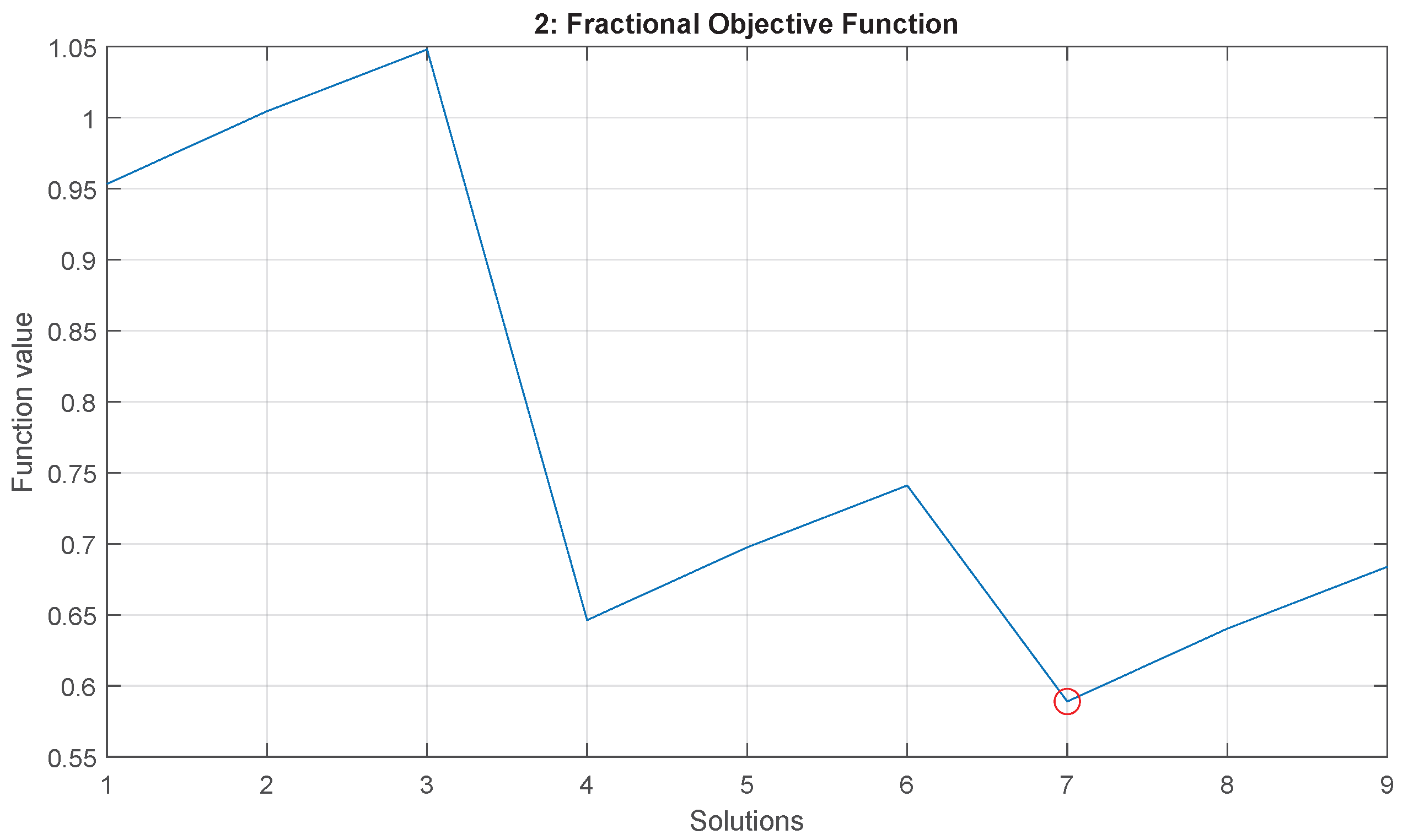
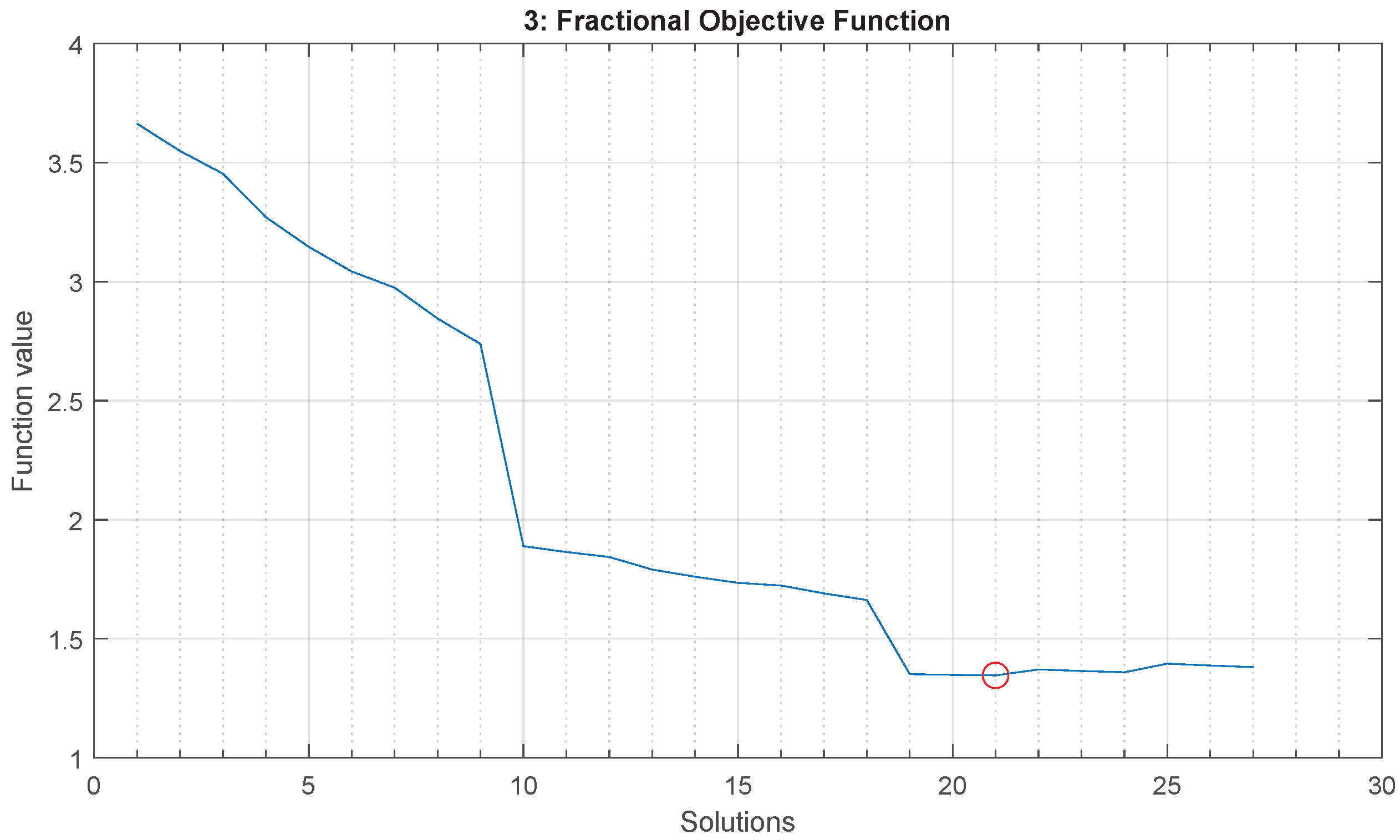
4.3.1. Fractional Objective Function

Using the expression for the stress in a truss element, an objective function can be set up to describe the difference between the truss element stress and the maximum limit stress allowed by the material. If such a difference can be minimized, then the truss element will be as close as possible to the material’s limit stress, meaning that the material is used optimally and the weight of the truss is implicitly minimized.

When setting up the objective function, it is important to consider that the truss element stress evaluates to a negative number under compression. However, because it is not known beforehand which truss elements will experience compressive or tensile stresses, this poses an issue. It is not possible to apply an absolute function to the truss element stress, as such a mathematical function is incompatible with QUBO problem formulations. As an alternative, the expression for the truss element stress can be squared to ensure that it always evaluates to a positive number. To keep consistent units, this also means that the maximum allowable stress is squared. A minimization problem is obtained by squaring the difference between the squared material limit stress and the squared truss element stress. As such, for a single truss element n, a minimization objective function can be defined as shown in Equation (17).

$$F_n={\left({\sigma }_{\mathit{limit}}^2-{\sigma }_n^2\right)}^2$$

(17)

With Equation (17), the minimum solution should encode the choice of truss cross-sectional area that minimizes the absolute difference between the material limit stress and the truss stress. To set up an objective function that describes the entire system of truss elements, the summation is taken over the objective functions of all truss elements, which leads to Equation (18).

$$F=\sum _{n=1}^N{F}_n=\sum _{n=1}^N{\left({\sigma }_{\mathit{limit}}^2-{\sigma }_n^2\right)}^2$$

(18)

Equation (18) gives a general expression for the objective function of each of the sample problems. It is important to note that, because the truss element stresses ${\sigma }_n$ are fractional in nature, as was shown in Equations (14)–(16), the objective function from Equation (18) will also have a fractional form. Hence, the resulting objective function is referred to as the fractional objective function. The fractional objective function was set up for each of the three sample problems, and was evaluated by a brute-force analysis, i.e., it was evaluated at every possible solution. The results for the three sample problems are shown in Figure 4, Figure 5 and Figure 6. They are produced using the Matlab code which is available online [31]. The following global minimum solutions are found:

• Two-truss problem: minimum at solution number 7, $\left[0,0,1,1,0,0\right]$
• Three-truss problem: minimum at solution number 21, $\left[0,0,1,1,0,0,0,0,1\right]$
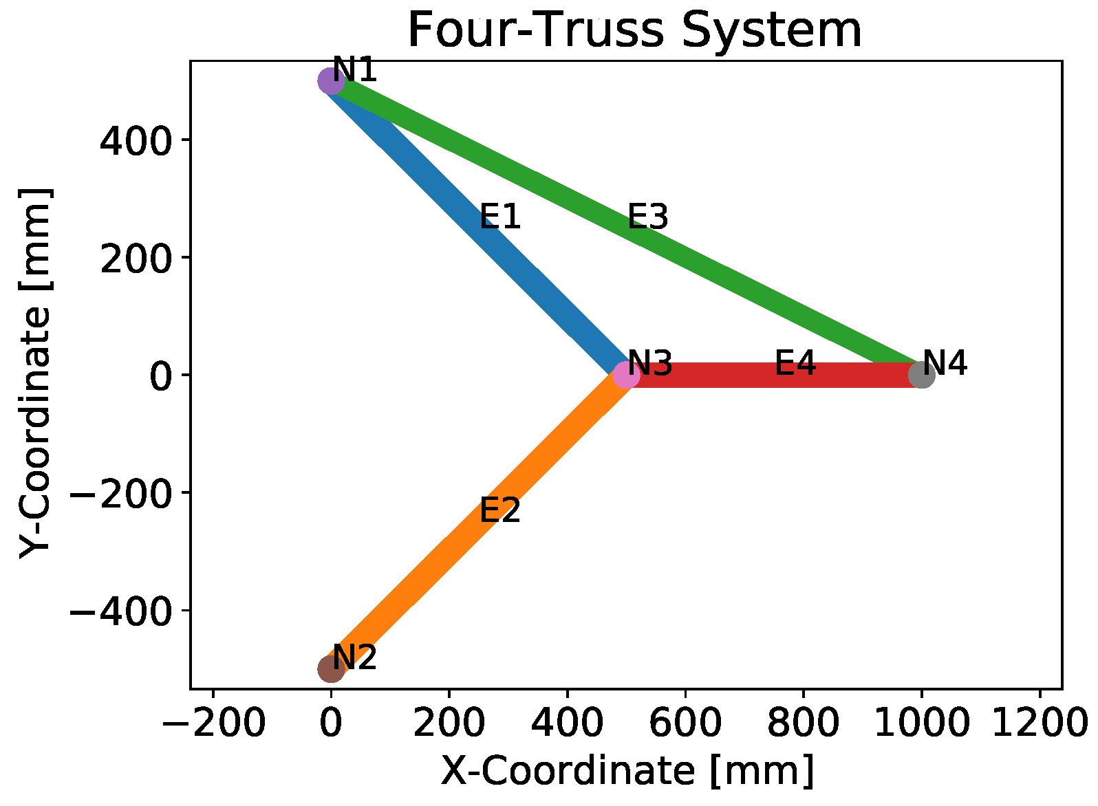
• Four-truss problem: minimum at solution number 7, $\left[1,0,0,1,0,0,0,0,1,1,0,0\right]$

The above brute-force results are used as references to benchmark the performance of the QA. One may be tempted to directly send the objective function in Equation (18) to the QA and see how it performs. However, one challenging aspect remains: the function has a fractional form. Fractional objective functions are incompatible with the QUBO formulation, and cannot be directly solved by the QA. As a result, in the next section, a method is investigated where a potential non-fractional objective function can be formed to approximate the original fractional one.

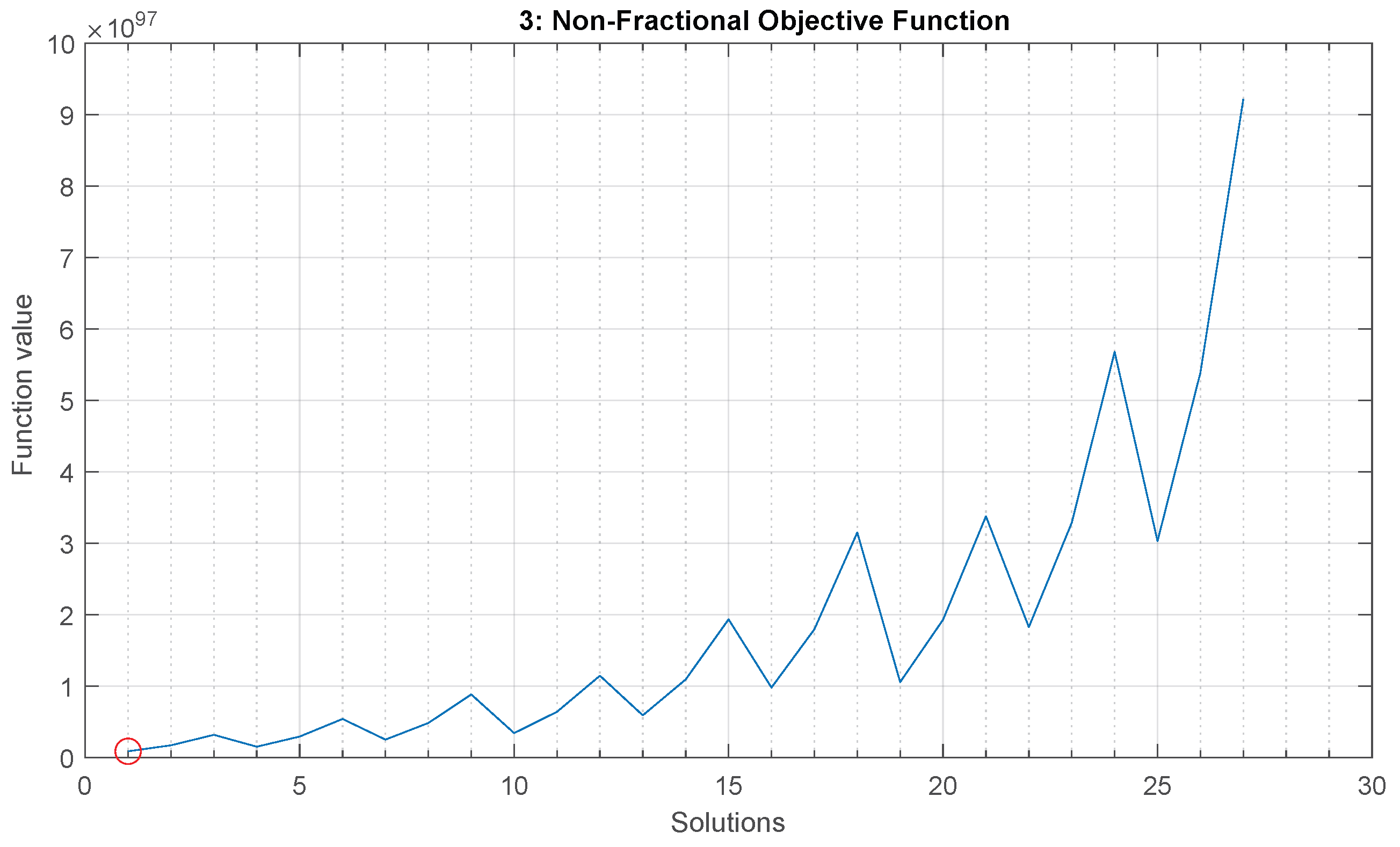
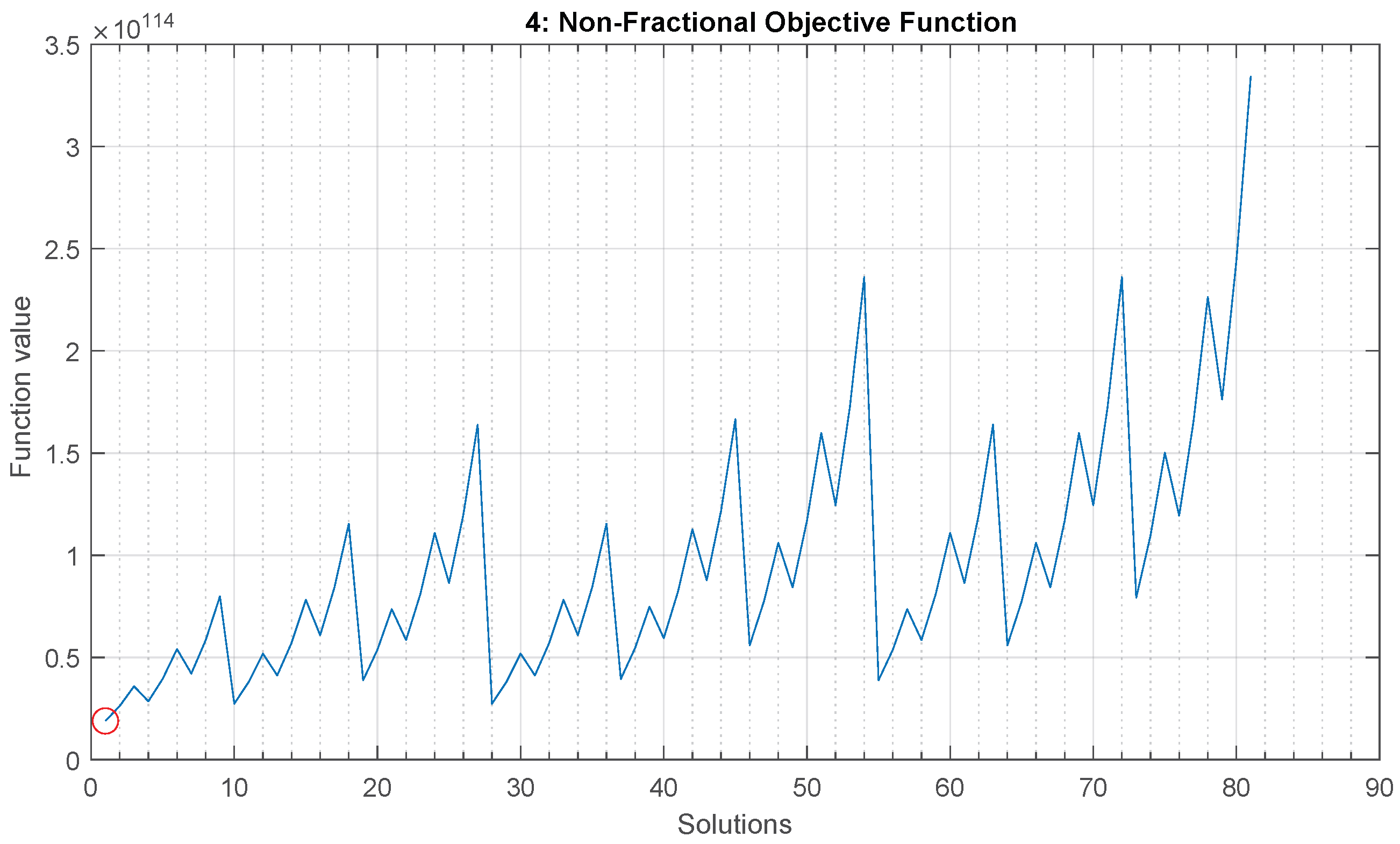
4.3.2. Non-Fractional Objective Function

In a QUBO-based objective function, only a summation of linear and quadratic terms is allowed. Therefore, in this section a potential method is investigated to formulate a non-fractional objective function for the discrete truss sizing optimization problem.

The reserve factor of a truss element gives a measure of how close the truss element is to material failure. The reserve factor for a truss element n is calculated via Equation (19).

$$R{F}_n=\frac{{\sigma }_{\mathit{limit}}}{|{\sigma }_n|}$$

(19)

To mitigate the absolute function for compatibility with QUBO, the material limit stress ${\sigma }_{limit}$ and truss element stress ${\sigma }_n$ can be squared, allowing a squared reserve factor can be calculated, according to Equation (20).

$$R{F}_n^2=\frac{{\sigma }_{\mathit{limit}}^2}{{\sigma }_n^2}$$

(20)

Using Equation (20), the theoretical optimal value of the squared reserve factor shall be 1 if the cross-sectional area can be varied arbitrarily. Given that the squared reserve factor is written as a fraction, this means that the numerator and the denominator should be equal to each other in the optimal case. In this case the numerator minus the denominator should also yield a result of zero. However, assuming that the currently known symbolic expression for the truss reserve factor actually describes a sub-optimal case, this will result in an error term. An optimization problem can then be set up for which the goal is to minimize this error by simply squaring the expression. This ensures that the optimum solution will be the one where the squared error is closest to zero, giving an objective function to minimize. The steps of this process are shown in Equation (21).

$$\begin{array}{cc}\hfill \mathrm{If}:& R{F}_n^2=\frac{{\sigma }_{\mathit{limit}}^2}{{\sigma }_n^2}\mathrm{and}{\sigma }_n^2=\frac{{\sigma }_{N,n}^2}{{\sigma }_{D,n}^2}\hfill \\ \hfill \mathrm{Rewriting}:& R{F}_n^2=\frac{{\sigma }_{\mathit{limit}}^2{\sigma }_{D,n}^2}{{\sigma }_{N,n}^2}=\frac{N_n}{D_n}\hfill \\ \hfill \mathrm{When}:& R{F}_n^2=\frac{N_n}{D_n}=1\hfill \\ \hfill \mathrm{Then}:& N_n=D_n\hfill \\ \hfill \mathrm{Optimally}:& N_n-D_n=0\hfill \\ \hfill \mathrm{Sub}-\mathrm{optimally}:& N_n-D_n=ϵ\hfill \\ \hfill \mathrm{Optimizing}:& min\left({ϵ}^2\right)\Rightarrow min\left({\left(N_n-D_n\right)}^2\right)\hfill \end{array}$$

(21)

With the above reasoning, the non-fractional objective function for a truss element n is written in Equation (22).

$$F_n={(N_n-D_n)}^2={\left({\sigma }_{\mathit{limit}}^2{\sigma }_{D,n}^2-{\sigma }_{N,n}^2\right)}^2$$

(22)

The objective function for the complete truss system is then found by taking the sum for all truss elements, as given in Equation (23).

$$F=\sum _{n=1}^N{F}_n=\sum _{n=1}^N{\left({\sigma }_{\mathit{limit}}^2{\sigma }_{D,n}^2-{\sigma }_{N,n}^2\right)}^2$$

(23)

This reformulated non-fractional objective function was also tested on the sample problems, using the brute-force method [31], to see if the minimum solutions would remain the same as those of the original fractional objective function. The results of these analyses are shown in Figure 7, Figure 8 and Figure 9, with the global minimum solutions indicated with small red circles. The following global optimum solutions are obtained:

• Two-truss problem: minimum at solution number 7, $\left[0,0,1,1,0,0\right]$
• Three-truss problem: minimum at solution number 1, $\left[1,0,0,1,0,0,1,0,0\right]$
• Four-truss problem: minimum at solution number 1, $\left[1,0,0,1,0,0,1,0,0,1,0,0\right]$

Using the non-fractional objective function, the expected solution for the two-truss problem is returned. However, for the three- and four-truss problems, the results are not those expected. Therefore, this method is presumed to be flawed. In this method, the difference between $N_n$ and $D_n$ is considered, rather than their ratio. A solution that minimizes the difference between $N_n$ and $D_n$ may not be the same as the one for which the ratio between $N_n$ and $D_n$ is closest to 1. Hence, this may be the source of the flawed results produced by this non-fractional objective function. In the next section, an alternative method is employed, with which a fractional objective function can still be made compatible with the QA.

4.4. Iterative Non-Fractional Approximations to the Fractional Objective Function

Ajagekar et al. have developed a method with which the optimum solution to fractional objective functions can be found by iteratively solving an adaptive non-fractional function [32]. The iterative scheme described by the authors is presented in Equation (24).

$$\begin{array}{cc}\hfill \mathrm{With}:& F=\frac{N\left(\mathbf{q}\right)}{D\left(\mathbf{q}\right)}\hfill \\ \hfill 0:& \mathrm{Initialize}\mathrm{variables}\hfill \\ \hfill & \mathit{iter}=0\hfill \\ \hfill & \lambda =0\hfill \\ \hfill & \mathit{obj}=\infty \hfill \\ \hfill & \delta ={10}^{-6}\hfill \\ \hfill 1:& \mathbf{while}\left|\lambda -obj\right|>\delta \hfill \\ \hfill 2:& \mathit{iter}=\mathit{iter}+1\hfill \\ \hfill 3:& F_{nf}\left(\mathbf{q}\right)=N\left(\mathbf{q}\right)-\lambda D\left(\mathbf{q}\right)\hfill \\ \hfill 4:& \mathrm{find}\widehat{\mathbf{q}}\mathrm{s}.\mathrm{t}.min\left(F_{nf}\left(\widehat{\mathbf{q}}\right)\right)\hfill \\ \hfill 5:& \mathit{obj}=\lambda \hfill \\ \hfill 6:& \lambda =F\left(\widehat{\mathbf{q}}\right)\hfill \end{array}$$

(24)

In this scheme, the fractional objective function $F\left(\mathbf{q}\right)$, expressed in terms of the binary problem variables $\mathbf{q}$, is rewritten into a non-fractional form. This happens in step 3 of the scheme, where the non-fractional objective $F_{nf}\left(\mathbf{q}\right)$ is formed. If this non-fractional function can be written in a QUBO form, then its optimal solution $\widehat{\mathbf{q}}$ can be found using the QA in step 4. In step 6, the objective function value of the original fractional function is evaluated using $\widehat{\mathbf{q}}$. When the difference between the objective function values found in consecutive iterations is less than $\delta$, the while loop is broken and the analysis has converged. Ultimately, the final solution that is found for $\widehat{\mathbf{q}}$ will be the minimum solution to the original fractional objective function.

The above-mentioned method has been implemented in Python scripts for the discrete truss sizing optimization problems [31]. Here, the method has been slightly extended, to include a user-defined maximum number of iterations. This has been added as an additional condition to the while loop in step 1 of Equation (24). In other words, step 1 is defined as:

$$\mathbf{while}\left|\lambda -obj\right|>\delta AND\mathit{iter}\le {\mathit{iter}}_{max}$$

(25)

Setting a maximum number of iterations will help prevent wasting excessive quantum computational time in cases where the analysis has difficulty converging on an optimal solution.

4.5. Objective Function Processing to Yield a QUBO Problem

With the iterative scheme by Ajagekar et al. [32], the solution to the fractional objective function for the discrete truss sizing optimization problem can be found by iteratively minimizing an adaptive non-fractional function. Once this non-fractional form is determined, there are a number of processing and simplification steps to take to eventually transform it into a QUBO form. By reducing the complexity of the objective function, the QA might be able to more easily identify the global optimum solution. The processing steps will allow the user to fine-tune the performance of the QA and to aid in finding valid solutions to the problem. In the following sections, the simplifications and processing steps are discussed.

4.5.1. High-Order Truncation

The first simplification to the rewritten non-fractional objective function is to truncate the excessively high-order terms. Specifically, for a system with N truss elements, any term in the objective function that is above $N^{\mathrm{th}}$ order can be truncated, since for a valid solution to the truss optimization problem, only N qubits are expected to end in a 1 state, while all other qubits should end in a 0 state. Therefore, all terms in the objective function that are above $N^{\mathrm{th}}$ order do not contribute to valid solutions. These terms can, therefore, be safely truncated to simplify the overall objective function without any influence on the validity of the solution.

The objective functions generally contain every possible unique multiplication between the qubit variables. Therefore, truncating the excessively high-order terms from the objective function can have a very large impact on the overall complexity of the objective function. This was investigated with a simple Excel sheet, which is made available online [31]. For example, in the two-truss problem, a total of six qubit variables are used. In total, this gives 63 different unique multiplications of qubit variables from first to sixth order. For this problem, all terms above second order only contribute to the invalid solutions, as valid solutions are expected to have exactly two qubit variables with a value of 1. Therefore, terms above second order can all safely be removed from the objective function. After truncating the terms above second order, only 21 total first- and second-order terms remain in the objective function, resulting in a 66% reduction in the number of terms in the objective function. In a similar vein, for the three-truss problem, this truncation reduces the number of terms in the objective function by roughly 75%. For the four-truss problem, the reduction is approximately 80%. It is expected that such a significant reduction in the complexity of the objective function will allow the QA to more easily find valid global minimum solutions to the truss sizing optimization problems.

4.5.2. Linear Scaling

When submitting problems to the QA, there are a number of parameters that can be fine-tuned to alter or improve the performance of the QA. The relative magnitudes of these parameters are typically what matters to the performance of the QA. To set a consistent baseline for solving the truss sizing optimization problems, it is, therefore, convenient to scale the magnitude of the objective function to a user-defined value. In this way, the magnitude of other constraints can be scaled accordingly. Thus, a linear scaling of each of the terms in the objective function can be performed, to ensure that the terms have consistent and controllable magnitudes.

First of all, the term with the maximum absolute magnitude in the objective function, $c_{\mathit{max}}$, must be found. Then, every term in the objective function F can be divided by this magnitude to perform the linear scaling. A user-defined parameter, $c_{\mathit{user}}$, is introduced to ensure that the maximum magnitude of the terms in the objective function can be exactly specified. Thus, the linear scaling of the objective function F is performed as shown in Equation (26).

$$F_{scaled}=\frac{c_{\mathit{user}}\times F}{c_{\mathit{max}}}$$

(26)

Inside the linearly scaled objective function $F_{scaled}$, the term with the maximum magnitude will have a magnitude of $c_{user}$. By altering the value of $c_{\mathit{user}}$, the user is able to control the relative importance of the objective function with respect to other problem-specific parameters such as constraints.

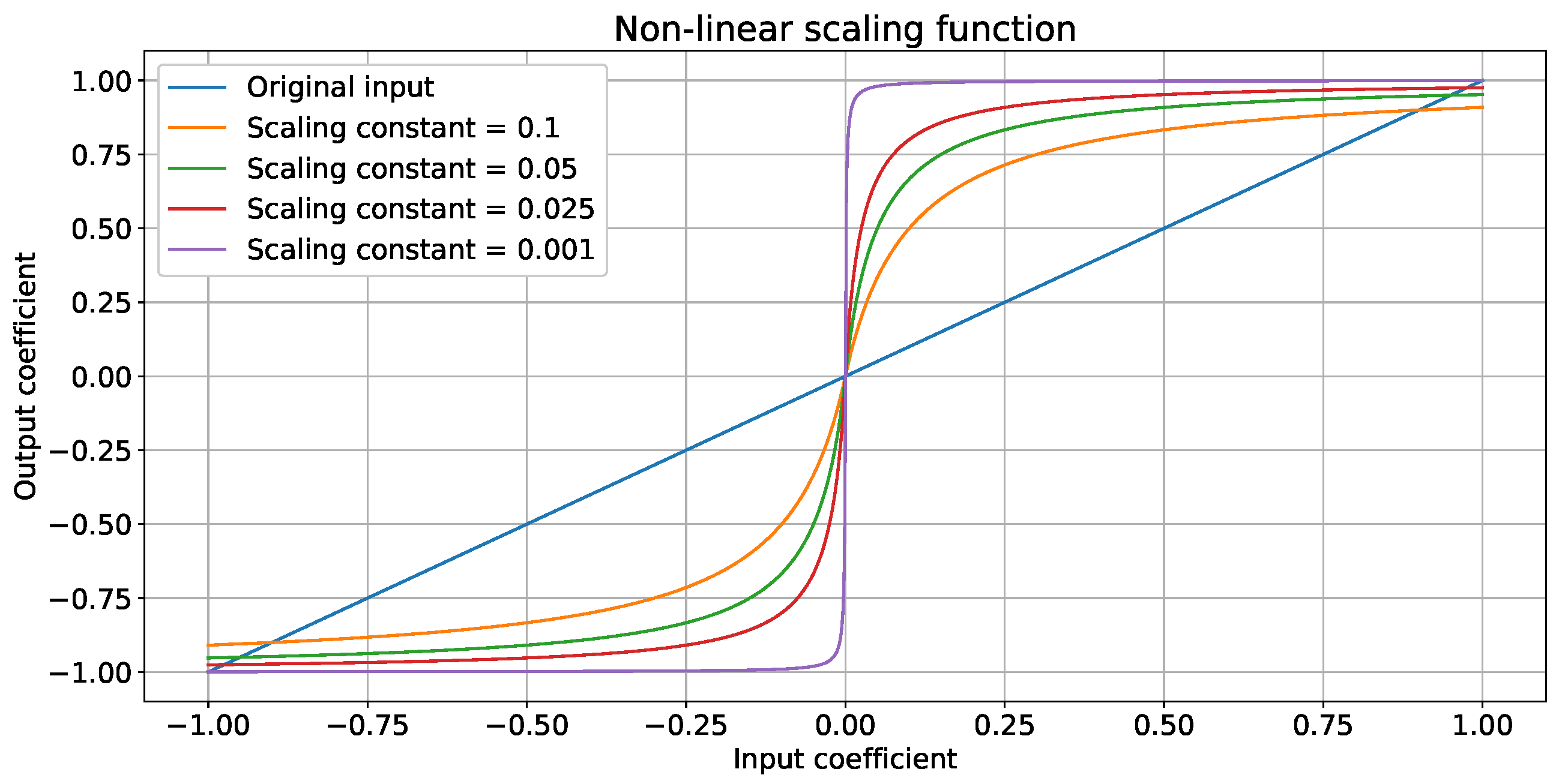
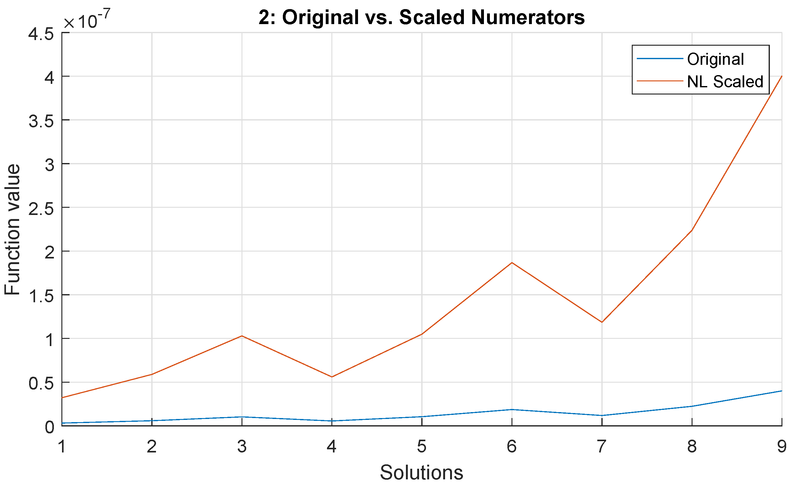
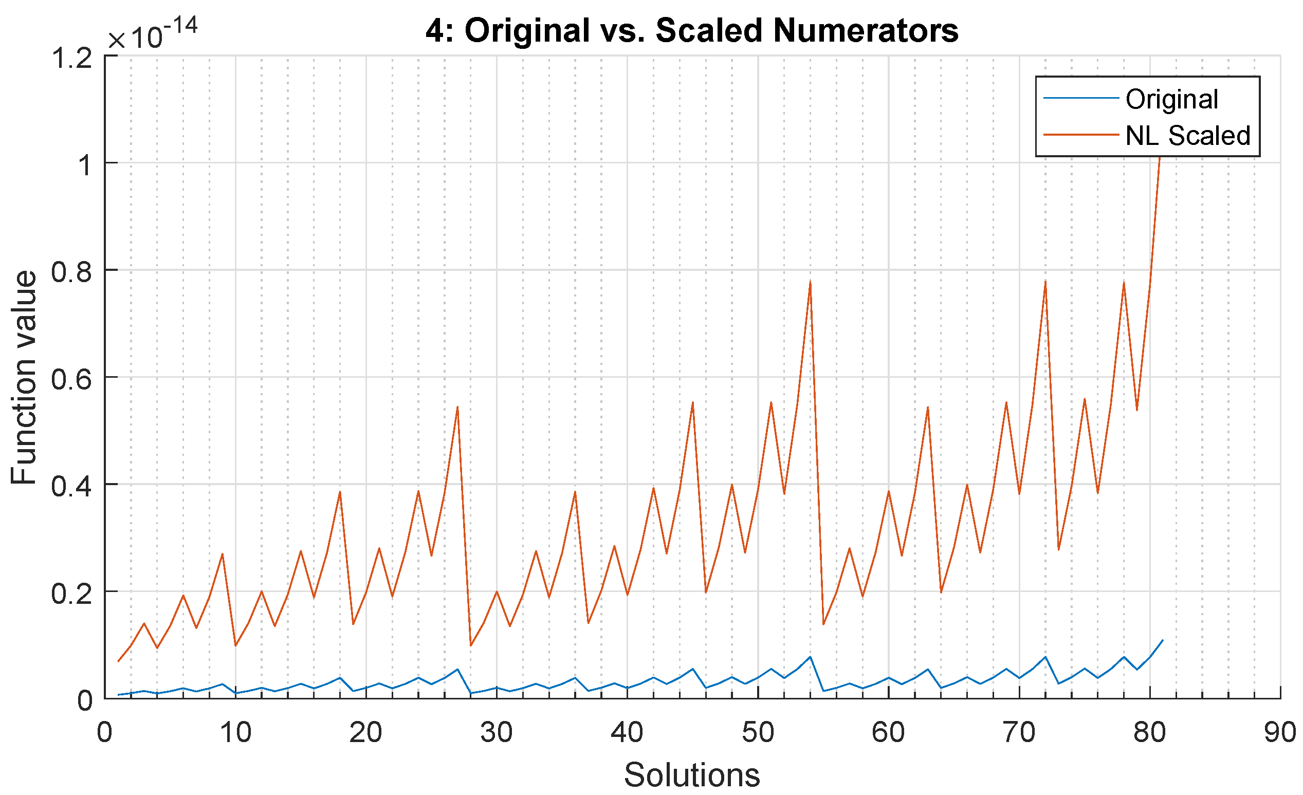
4.5.3. Non-Linear Scaling

During the brute-force testing of the objective functions for the different sample problems in Section 4.3, it was seen that with certain objective functions the global minimum solution and other local minimum solutions can have nearly identical function values. This was especially the case for the three-truss problem with the original, fractional objective function. When the differences between solutions are small, it becomes difficult for the QA to find the global optimum solution. The very small differences between local minima and the global minimum are mainly due to some terms in the objective function having very small, high-precision coefficients.

Due to analog control errors, small and high-precision coefficients are difficult for the QA to correctly take into account [33]. Furthermore, when a problem is submitted to the D-Wave QA, it is by default automatically scaled (by auto_scale) to ensure the problem coefficients fall inside the controllable range of the QA. For linear QUBO coefficients, this range is between −2 and 2. For the quadratic QUBO coefficients, the maximum available range is between −2 and 1 [34]. By default, the QA uses a range between −1 and 1. These ranges can be directly queried from the D-Wave solver using Python commands:

                         DWaveSampler().properties[’h_range’]

                         DWaveSampler().properties[’j_range’]

It is good to be mindful of this automatic scaling before submitting problems to the QA to prevent cases where a problem is unexpectedly scaled down to a magnitude that cannot feasibly be controlled by the QA.

To assist the QA with small high-precision coefficients, it would be beneficial if these coefficients could be amplified. In turn, this might also amplify the differences between the global and other local minimum solutions. This would potentially help the QA find the global optimum solution. Furthermore, this would also help the QA more effectively utilize information from the objective function, as previously insignificant terms might be amplified to a magnitude that the QA could actually take into account. With this idea in mind, a non-linear scaling method has been developed, with which very small coefficients in the objective function can be scaled to become larger and more influential, while terms that are already significant are not scaled as much.

A Python function has been created to perform this non-linear scaling. The method relies on simple user-defined parameters which allow for manual tweaking once the objective function has been fully implemented for use on the QA. Given the user-defined scaling parameter $c_{\mathit{NL}}$, a positive coefficient $c_{\mathit{in}+}$ from the objective function is input into the non-linear scaling function. The non-linearly scaled coefficient $c_{\mathit{out}+}$ is then expressed by Equation (27).

$$c_{\mathit{out}+}=\frac{c_{\mathit{in}+}}{c_{\mathit{in}+}+c_{\mathit{NL}}}$$

(27)

For negative input coefficients, $c_{\mathit{in}-}$, the non-linear scaling is performed by Equation (28), yielding the negative non-linearly scaled coefficient $c_{\mathit{out}-}$.

$$c_{\mathit{out}-}=-\frac{c_{\mathit{in}-}}{c_{\mathit{in}-}-c_{\mathit{NL}}}$$

(28)

To determine if the input coefficient must be scaled using either Equation (27) or Equation (28), a simple if statement is used. By setting $c_{\mathit{NL}}$ to be a certain small number, such as 0.025, the amount of scaling applied to small coefficients is much higher than that applied to large coefficients.

As a demonstration of the non-linear scaling, several plots are given in Figure 10, showing the influence of changing the parameter $c_{\mathit{NL}}$. It can be seen that the scaling is much more significant for smaller coefficients than for larger ones. However, with very aggressive values of $c_{\mathit{NL}}$, such as 0.001, this can also cause all relatively large coefficients to become essentially equal. The use of this non-linear scaling function will, therefore, be a balancing act of increasing the importance of smaller coefficients without losing the distinction between the larger ones. The Python code for the non-linear scaling function, and for producing the plot from Figure 10, is available online [31].

The effect of the non-linear scaling was also investigated for the specific truss sizing sample problems. The non-linear scaling was performed during the iterative solving procedure. Specifically, it was performed between steps 3 and 4 of the procedure outlined in Equation (24), and was applied to the rewritten non-fractional objective function. The effect of the non-linear scaling was investigated for the first iteration of the sample problems. This first iteration is convenient to investigate as Equation (24) shows that $\lambda =0$, meaning that the objective function in step 3 in Equation (24) only involves the numerator of the original fractional objective function. The rewritten non-fractional function was firstly linearly scaled, choosing the user-defined maximum coefficient to be $c_{\mathit{user}}=1$. This brought the function values to a reasonable range for the QA. Then, the non-linear scaling was applied, using a scaling parameter of $c_{\mathit{NL}}=0.1$. The plots in Figure 11, Figure 12 and Figure 13 show both the original (linearly scaled) and non-linearly scaled energy landscapes of the first iteration in the solving procedure for the sample truss problems. It can be seen that the small fluctuations in the energy landscape are amplified, which should make the problem easier to solve for the QA. Therefore, the non-linear scaling has been applied when submitting problems to the QA.

It is important to note that this non-linear scaling method is developed solely for the purpose of increasing the differences between the global and local minima in the energy landscapes of this study. It is not intended to be used as a general-purpose tool for problems with unknown energy landscapes, since using overly aggressive scaling factors for $c_{\mathit{NL}}$ may cause the global minimum solution to change. However, this is not expected to be an issue for the truss sizing optimization problems here. In step 6 of the iterative solving procedure in Equation (24), the interim solution $\widehat{\mathbf{q}}$ is evaluated with the original fractional objective function, meaning that the iterative procedure should eventually converge on the global optimum of the original fractional objective function.

4.5.4. Truncation of Insignificant Terms

Once the linear and non-linear scaling has been performed, it is possible to further simplify the objective function. After all the scaling has been applied, certain terms in the objective function may still have magnitudes very close to zero. Such terms would be difficult for the QA to consider as there is a finite precision with which qubit biases can be controlled within the QA hardware [33]. If the magnitudes of the terms in the objective function were smaller than the analog control error of the QA for the qubit biases, they would not be reliably taken into account by the QA. Thus, terms that are too small in magnitude can simply be removed from the objective function, as including them is akin to simply introducing noise into the function. A conservative truncation approach is to remove terms with magnitudes smaller than ${10}^{-8}$, which is beyond the precision that the QA can control. This reduces the complexity of the objective function, facilitating the QA in finding the global optimum solution.

4.5.5. Unary Constraint

The majority of the solutions to the truss optimization problems are invalid, i.e., when an incorrect number of cross-sectional areas are selected. In other words, when either zero or more than one cross-section is selected for a truss member, the solution is invalid. Solutions can only be valid when exactly one cross-sectional area is chosen for every truss member. To promote the selection of valid solutions, the unary constraint is implemented.

For every truss element n in a truss system, with a total of C possible choices of cross-sectional area, Equation (29) must hold for valid solutions to the truss sizing optimization problem.

$$\sum _{c=1}^C{q}_{n,c}=1$$

(29)

Since only one of the qubits on which this constraint acts can take a value of 1, while the others must all equal 0, this constraint is, therefore, referred to as the unary constraint. Further elaboration on the unary constraint is given in [35]. In the context of the truss optimization problem, it enforces that only one cross-section is chosen per truss element. However, in the form shown in Equation (29), the constraint cannot be directly applied in the QUBO problem framework because it is written as an equality constraint, which by definition is incompatible with the quadratic unconstrained binary optimization format. For the constraint to become QUBO-compatible, it must be rewritten as an objective function of a minimization problem. A common method is to rewrite the equality constraint as a penalty function using a ‘squared-error’ approach [36,37]. This approach is also used, for example, in the work of Van Vreumingen et al. and Neukart et al. [10,11]. Here, the constraint can be rewritten as shown in Equation (30).

$$\begin{array}{c}\hfill \left(\sum _{c=1}^C{q}_{n,c}\right)-1=0\\ \hfill {\left(\left(\sum _{c=1}^C{q}_{n,c}\right)-1\right)}^2=0\end{array}$$

(30)

Now, adding in a penalty scaling factor $\lambda$, the Hamiltonian energy penalty function for the unary constraint becomes:

$$\begin{array}{c}\hfill H_U=\lambda {\left(\left(\sum _{c=1}^C{q}_{n,c}\right)-1\right)}^2\end{array}$$

(31)

For the truss sizing optimization problems, only three possible choices of cross-sectional area are available per truss element, i.e., $C=3$. Therefore, Equation (31) can be expanded and simplified, as shown in Equation (32).

$$\begin{array}{cc}\hfill H_U=& \lambda \left(q_{n,1}+q_{n,2}+q_{n,3}-1\right)\left(q_{n,1}+q_{n,2}+q_{n,3}-1\right)\hfill \\ \hfill H_U=& \lambda \left(q_{n,1}^2+q_{n,1}{q}_{n,2}+q_{n,1}{q}_{n,3}-q_{n,1}\right.\hfill \\ \hfill & +q_{n,1}{q}_{n,2}+q_{n,2}^2+q_{n,2}{q}_{n,3}-q_{n,2}\hfill \\ \hfill & +q_{n,1}{q}_{n,3}+q_{n,2}{q}_{n,3}+q_{n,3}^2-q_{n,3}\hfill \\ \hfill & \left.-q_{n,1}-q_{n,2}-q_{n,3}+1\right)\hfill \end{array}$$

(32)

Knowing that $q_{n,c}\in \left\{0,1\right\}$, which means that $q_{n,c}^2=q_{n,c}$, the expression can be further simplified:

$$\begin{array}{cc}\hfill H_U=& \lambda \left(2q_{n,1}{q}_{n,2}+2q_{n,2}{q}_{n,3}+2q_{n,1}{q}_{n,3}-q_{n,1}-q_{n,2}-q_{n,3}+1\right)\hfill \end{array}$$

(33)

Finally, the constant term can be dropped, since it is independent of the qubit variables, and does not affect the minimization problem. This makes the unary constraint penalty function compatible with the QUBO problem framework, since it can now be written as a pure summation of linear and quadratic terms, as shown in Equation (34).

$$\begin{array}{cc}\hfill H_U=& \lambda \left(2q_{n,1}{q}_{n,2}+2q_{n,1}{q}_{n,3}+2q_{n,2}{q}_{n,3}-q_{n,1}-q_{n,2}-q_{n,3}\right)\hfill \end{array}$$

(34)

By adding the unary constraint of each truss element to the overall objective function, the QA is more likely to find valid solutions. The strength of the unary constraint can be fine-tuned by altering the value of the user-defined parameter $\lambda$. By trial and error, it has been found that a good starting value of $\lambda$ is twice the magnitude of the maximum term in the objective function. However, if invalid solutions are consistently found, the strength of the constraint can be increased until noncompliance with the constraint stops occurring.

4.5.6. Quadratization

Up until this point, the objective function has been manipulated, scaled, and truncated in order for it to become more compatible with the QUBO problem formulation. However, one key issue has yet to be solved: the function may still contain many terms that are higher than second order. Therefore, it still cannot be used on the QA, since by definition the QA can only solve quadratic problems. Performing a quadratization of a high-order objective function ensures that it is rewritten as a quadratic function with equivalent solutions.

There are many different methods of quadratization in literature. An extensive overview on the topic is given by Dattani [38]. Some of these methods utilize auxiliary variables to rewrite the high-order objective function into an equivalent quadratic-order expression, while others achieve this without the auxiliary variables. Each method has its respective benefits and drawbacks. For example, it is convenient when no auxiliary variables are needed, yet in that case it may require much more effort to rewrite the objective function in an equivalent quadratic form. Alternatively, if a method uses auxiliary variables, it may be easier to find an equivalent quadratic form, but the additional variables would increase the complexity of the objective function, making it more difficult for the QA to find the optimum solution [38].

The quadratization has already been implemented in D-Wave [39]. In their implementation, all the high-order terms of the objective function are rewritten and replaced by auxiliary variables, such that the final expression is at most quadratic. An additional user-defined parameter is used to select the strength with which the quadratization is enforced [39]. If the quadratization is not enforced correctly, this can result in a poor approximation of the original high-order objective function. The quadratization strength is problem-dependent and must be tuned such that the quadratization is always obeyed, so as to have an accurate representation of the original high-order objective function.

With the quadratization, the discrete truss sizing optimization problems can finally be written as QUBO problems. This vital step concludes all the necessary preparatory work for the problems to be made compatible with the quantum computing hardware. They can now be solved using the D-Wave QA. In the next section, some notable parameters that influence the solution process of the QA are discussed.

4.6. Parameter Tuning

In the previous sections, a number of user-defined parameters have been introduced which influence the objective functions of the three truss sizing problems. Their values need to be chosen before the problems can be submitted to the QA. In summary, values for the following parameters need to determined:

• Iterative solving procedure

  -

  Maximum number of iterations allowed

  -

  Iteration convergence threshold

• Objective function processing

  -

  Highest order terms allowed

  -

  Linear scaling magnitude

  -

  Non-linear scaling strength

  -

  Precision truncation magnitude

  -

  Unary constraint strength

  -

  Quadratization strength

• Quantum annealing

  -

  Number of reads

  -

  Chain strength

To aid in finding sensible values for most of the above parameters, without wasting the limited amount of quantum computational time available, an alternative classical solver was used before running on the QA. D-Wave provides a simulated annealing (SA) algorithm, which can be used to solve QUBO problems. The SA solver only relies on the local classical computing hardware and does not expend any of the quantum computational time allowance. The SA solver was, therefore, used first to test the functionality of the Python code, and to find initial values for the relevant problem parameters.

Values for the parameters related to the iterative solving procedure were determined first. Testing via the initial SA analyses showed that around five iterations were needed to find a converged solution. This value was tripled for the quantum annealing analyses to give enough room for the iterations to converge. Thus, the maximum number of iterations within one solving attempt was set to 15. If the procedure could not converge after the maximum number of iterations was reached, the analysis would be stopped to prevent excessive expending of computational time. The convergence threshold $\delta$ for the iterative procedure (as seen in Equation (24)) was set to ${10}^{-6}$, the same as the one used by Ajagekar et al. [32].

Starting values for the different objective function processing parameters were also determined from the initial SA analyses. First of all, the highest order of terms allowed in the objective function for each of the sample problems was set equal to the number of truss elements. Second, the linear scaling maximum magnitude $c_{\mathit{user}}$ was set to a value of 1 for all analyses. Third, the non-linear scaling parameter $c_{\mathit{NL}}$ was set to a value of 0.1 for all analyses. During the brute-force testing, it was observed that this value improved the distinction between minima in the energy landscapes of the sample problems, while preserving the location of the global minima. Fourth, the unary constraint strength was set to a value of 10 for the two- and three-truss problems. For the four-truss problem it was set to a value of 20. Testing via SA showed that with these settings the constraint was obeyed consistently, yielding valid solutions to the truss sizing problems. Fifth, terms that had a magnitude smaller than ${10}^{-8}$ were truncated to slightly reduce the number of terms in the objective functions. This is a conservative truncation as it is well beyond the precision that the QA hardware can control. Finally, the quadratization strength was set to a value of 10 for the two- and three-truss problems, and a value of 20 for the four-truss problem, such that it could match the strength of the unary constraint.

For the QA, some additional parameters are needed to solve the sample problems. The number of reads describes the number of times a specific problem is solved by the QA before the final best-performing solution is returned to the user. Increasing the number of reads increases the likelihood of obtaining optimal solutions at the expense of additional computational time. To minimize the expenditure of quantum computational time, a viable number of reads needs to be firstly estimated.

Using the SA solver, some test runs were firstly performed in which the numbers of reads were set to values of 16, 64, and 256, for each of the three sample problems. For the two-truss problem, the global optimum results were obtained every single time, regardless of the number of reads. For the three-truss problem, using 64 and 256 reads reliably gave optimal or near-optimal results. For the four-truss problem, only when setting the number of reads to 256 was the global optimum result reliably obtained. The settings for the number of reads for the QA analyses were, therefore, chosen based on the above tests. Namely, for the two-truss problem, the number of reads was set to 16 and 64. For the three-truss problem the number of reads was set to 64 and 256. Finally, for the four-truss problem, the number of reads was only set to 256.

The chain strength parameter for the QA relates to a physical issue called chain break, which can occur while the QA is solving problems. To explain the fine-tuning of the chain strength parameter, some context on the chaining of qubits is firstly given. A QUBO problem is defined through an upper-triangular $N\times N$ matrix $\mathbf{Q}$. The terms on the diagonal of the matrix $\mathbf{Q}$ relate only to a single problem variable, while the off-diagonal terms describe an interaction between two different variables. On the D-Wave 2000Q used in this research, each qubit can only directly interact with at most six other qubits [8]. This limited connectivity between qubits can present an issue for larger QUBO problems where more connectivity may be needed. When a QUBO is submitted to the QA, it must be embedded onto the physical architecture of the QPU. The embedding translates the logical structure of a QUBO problem to the physical structure of the QA. This also means that the logical problem variables are translated to the physical qubits on the QPU. However, when the QUBO problem necessitates a high connectivity between logical problem variables, it can become impossible to directly embed every logical variable onto an individual single qubit. By chaining together strings of multiple qubits and forcing them to act as single logical problem variables, the connectivity between the embedded logical variables can be increased beyond the limitations of the physical hardware [40].

In practice, problems can become very challenging for the QA to solve if the number of interactions between variables is high. A QUBO problem with high connectivity requirements will lead to embeddings with very long qubit chains. In turn, the longer the qubit chains are, the more difficult it is to force the chained qubits to act in unison. When a qubit chain is working as intended, the chained qubits will all end up in the same final ground state, i.e., all being either 0 or 1. However, when a qubit chain is broken, the qubits in the chain will end up in a mixture of 0 and 1 states. This makes the final state of the qubit chain and the intended final state of the corresponding logical problem variable unclear. By increasing the chain strength, the risk of chain breaks occurring is reduced. However, overly high chain strength should be avoided as the relative strength of the objective function itself is reduced, potentially making it more difficult to obtain the true global optimum solution.

In this work, a chain strength of 10 was selected initially, but it was seen that chain breaks would still occur for the three- and four-truss problems. For those problems a chain strength of 30 performed better, preventing chain breaks from occurring.

There are many additional parameters that can be tuned to alter the performance of the quantum annealer, but these are left in their default configurations [41]. In

Table 3. Parameters used for all analyses.

Parameters	Brute Force			Quantum Annealing
Truss system	2-truss	3-truss	4-truss	2-truss	3-truss	4-truss
Total number of times analyzed	3	3	3	10	10	10
Maximum number of iterations	NA	NA	NA	15	15	15
Iteration convergence threshold	NA	NA	NA	${10}^{-6}$	${10}^{-6}$	${10}^{-6}$
Number of reads per iteration	NA	NA	NA	$\left\{16, 64\right\}$	$\left\{64, 256\right\}$	$\left\{256\right\}$
Highest order terms allowed	NA	NA	NA	2	3	4
Linear scaling maximum magnitude	NA	NA	NA	1	1	1
Non-linear scaling strength	NA	NA	NA	0.1	0.1	0.1
Unary constraint strength	NA	NA	NA	10	10	20
Quadratization strength	NA	NA	NA	10	10	20
Precision truncation magnitude	NA	NA	NA	${10}^{-8}$	${10}^{-8}$	${10}^{-8}$
Chain strength	NA	NA	NA	10	30	30
Annealing time (μs)	NA	NA	NA	20	20	20

, a summary is given for all the parameters used in each analysis. Parameters that are irrelevant or not applicable for an analysis are indicated by NA.

5. Results

5.1. Overview of Analyses Performed

This section gives an overview of the performed analyses, of which results are reported in the following sections.

The fractional objective functions of the sample truss problems were firstly determined according to the methods described in Section 4.3. The times taken in this process were measured to gain insight into its efficiency and scalability.

Next, the brute-force evaluation of the original fractional objective functions was used to obtain baseline solutions. There are other more efficient (and more complicated) classical computing methods available for such problems, as reviewed by Stolpe [42], however, for the purposes of this study, the simple brute-force method is sufficient to produce the reference solutions as the problems are all small in size. Each of the brute-force analyses was performed three times so that an average solving time could be calculated.

The QA by D-Wave was then used to solve the problems using quantum annealing. Due to the probabilistic nature of the QA, it is not guaranteed that every analysis will yield the same solution. Therefore, for the given sample problems, each QA analysis was performed ten times. This allowed average computational times and standard deviations to be measured, together with the probability of obtaining the global optimum solution. The number of analyses could unfortunately not be increased due to limitations on the amount of quantum computational time allotted to basic user accounts on the D-Wave Leap platform.

The goal of performing these analyses is first to find out whether it is feasible to use quantum annealing to solve these practical truss optimization problems. Second, the gathered data on the computational times can give insights into the efficiency and scalability of the quantum annealing approach.

The specifications of the local classical computing hardware used in this research are given in

Table 4. Classical computing hardware.

Item	Specifications
Device	Lenovo Legion Y540-15IRH
CPU	Intel Core i7-9750H 2.6 GHz
Memory	16 GB DDR4 2667 MHz
GPU	Mobile NVIDIA RTX 2060 6 GB

.

5.2. Results: Two-Truss Problem

The two-truss problem is the simplest of the three sample problems. It took approximately 13.5 s to set up its fractional objective function. Once this objective function was found, it was written to a text file. The objective function was then imported whenever needed in the subsequent steps of the solution process and no longer needed to be set up from scratch. This saved some time when performing the three brute-force analyses. More importantly, for the QA, where ten analyses were performed with different numbers of reads, having the objective function ready significantly reduced the computational overhead.

For the brute-force analysis, when evaluating the fractional objective function for valid solutions, an average of 0.234 s was needed to find the global optimum solution. The baseline global optimum solution is $[0,0,1,1,0,0]$. This indicates the largest possible cross-sectional area should be chosen for the first truss element, while for the second truss element the smallest cross-sectional area should be chosen.

Using the QA, the analyses were performed ten times to gain some insight into the probability of obtaining the globally optimal solution. In Figure 14, the solutions obtained by the QA are presented in a histogram. Superimposed on the histogram is a line plot of the original fractional objective function previously calculated using the brute-force method.

It can be seen from Figure 14 that regardless of the choice for the number of reads, the QA finds solution number 7, which corresponds to the same global optimum solution as that obtained via the brute-force method.

When it comes to the computational time for the QA analyses, the following results were obtained:

• With number of reads = 16

  -

  Average total time = 19.52 s. Standard deviation = 5.10 s.

  -

  Average QPU time = 59,176 μs. Standard deviation = 15,061 μs.

• With number of reads = 64

  -

  Average total time = 19.06 s. Standard deviation = 0.21 s.

  -

  Average QPU time = 118,207 μs. Standard deviation = 10.7 μs.

From these results, it is seen that setting the number of reads to 64 leads to more consistent analysis times, as compared to using only 16 reads. On the other hand, by setting the number of reads to 64, the amount of QPU access time is increased significantly.

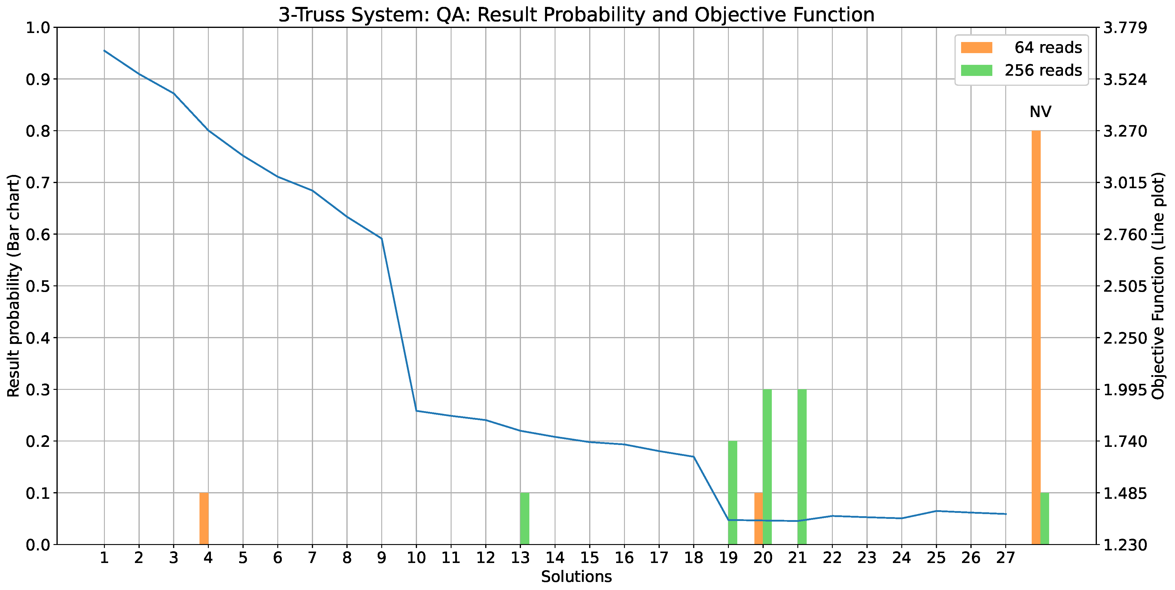
5.3. Results: Three-Truss Problem

The three-truss problem is a more complicated problem to set up compared to the two-truss problem, due to the increased number of variables. Setting up the fractional objective function for this problem and writing that expression to a text file took approximately 81.4 s.

Considering the brute-force analysis of the fractional objective function, it took an average of 0.9 s to find the global optimum solution $[0,0,1,1,0,0,0,0,1]$. This solution indicates that the largest cross-sectional area should be chosen for the first and third truss elements, and that the smallest cross-section should be chosen for the second truss element.

With the QA, the analyses were performed with the number of reads set to values of 64 and 256. The solution probability histogram in Figure 15 shows the results that were obtained. The figure also shows the original fractional objective function, as calculated via brute force. Analyses that ended with non-valid results are indicated by the ’NV’ column in the histogram.

From Figure 15, it can be seen that there is a large variation in performance depending on the setting for the number of reads. Setting the number of reads to 64 leads to non-valid solutions for most analyses. With this setting, the QA does not reliably produce usable results. However, when the number of reads is increased to 256, optimal or near-optimal valid solutions are obtained most of the time. From these results it is also clear that the problem is more difficult for the QA to solve as compared to the two-truss problem.

As part of the QA analyses, the following computational times were measured:

• With number of reads = 64

  -

  Average total time = 98.7 s. Standard deviation = 37.5 s.

  -

  Average QPU time = 337,477 μs. Standard deviation = 117,808 μs.

• With number of reads = 256

  -

  Average total time = 48.8 s. Standard deviation = 20.6 s.

  -

  Average QPU time = 558,414 μs. Standard deviation = 244,331 μs.

It is observed that setting the number of reads to 256 leads to more consistent behavior, as evidenced by the smaller standard deviation for the total analysis time. Furthermore, the higher number of reads allows for the analysis to converge more quickly, as fewer iterations are generally needed to find a solution. However, the consequence of choosing a higher number of reads is that the amount of QPU access time is also increased.

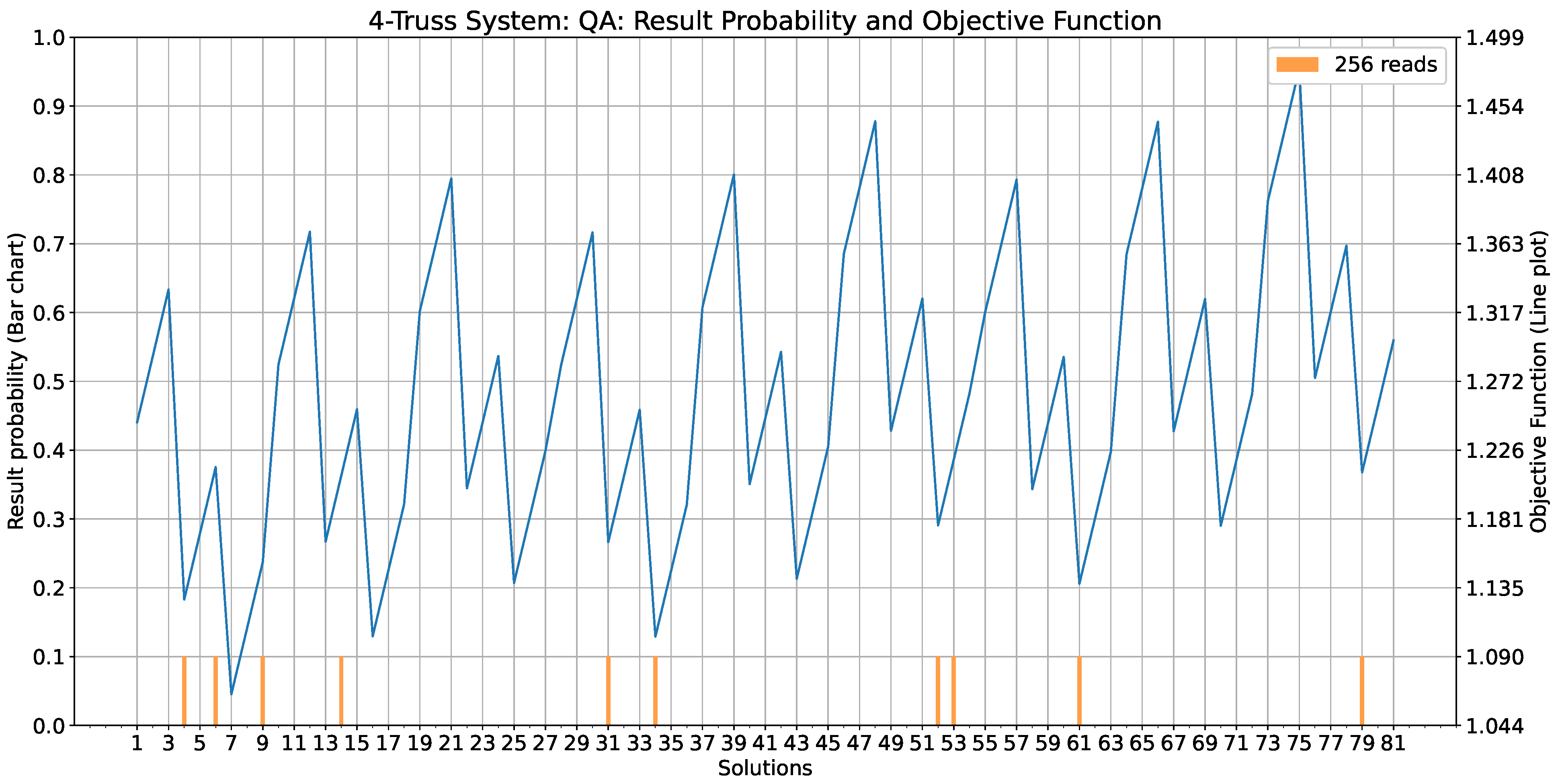
5.4. Results: Four-Truss Problem

The last problem, with the highest number of variables involved, is the four-truss problem. Using the symbolic finite element method, it took approximately 3431 s to set up the fractional objective function. This is a very significant increase from the roughly 81 s for the three-truss problem. In this case, it is a great benefit that the fractional objective function is written to a text file. Testing of the analysis procedures is much faster when the objective function text file can simply be imported and interpreted, as compared to prefacing every analysis by a nearly hour-long setup process.

Via brute-force analysis, the global optimum solution $[1,0,0,1,0,0,0,0,1,1,0,0]$ was found in an average of 4.4 s. This solution indicates that the first, second, and fourth truss elements should optimally use the smallest choice for the cross-sectional area. The third truss element should use the largest available cross-sectional area.

The histogram of the results that were obtained by the QA are shown in Figure 16. The figure also shows a line plot of the original fractional objective function, which was determined by the brute-force analyses.

From Figure 16, it is seen that seemingly random, but valid, solutions are obtained by the QA. Only one solution comes within 5% of the global optimum solution. Namely, solution number 34 was found once and it has an an objective function value of 1.103. The global optimum solution is located at solution number 7, and it has an objective function value of 1.065. It is worth noting that seven out of the ten analyses ended with an iteration run-out, rather than ending with a converged final solution.

The following computational time for the QA analyses was obtained:

• With number of reads = 256

  -

  Average total time = 437 s. Standard deviation = 39.0 s.

  -

  Average QPU time = 1,280,156 μs. Standard deviation = 251,109 μs.

The average solving time is approximately nine times longer than that for the three-truss problem, using the same number of reads. Furthermore, the average of 1.28 s of QPU access time per analysis meant that any further testing was not possible for this problem, as this would consume more than the 60 s monthly QPU access budget.

6. Conclusions

This work has established a new method to apply quantum annealing to the discrete optimization of truss structures. A symbolic FEM approach is employed to express the objective function in terms of qubit variables. As the qubit variables encode the design choices of the truss structure, they would inevitably take part in the formulation of the stiffness matrix of the structure, which leads to a fractional form for the objective function. Ajagekar et al’s iterative approach is used to approximate the original fractional objective function with a non-fractional one such that it can be made compatible with the QA. The proposed method has been applied on three discrete truss sizing optimization problems with increasing complexity. It is found that the QA is able to find the global minimum solution if sufficient reads can be afforded. However, there are several challenges that need to be addressed for this method to be scalable to larger problems.

6.1. Symbolic Finite Element Method

The first bottleneck is related to the symbolic finite element method used for the definition of the objective function in Section 4.3. The time to setup the objective function for each of the three sample problems was measured and is shown in

Table 5. Overview of objective function setup time.

Truss System	Variables	Setup Time (s)	Growth Factor
2	6	13.504	-
3	9	81.390	6.0270
4	12	3430.542	42.1494

.

The timings given in Table 5 show that the symbolic finite element method implementation scales poorly as the number of problem variables increases. Solving the symbolic finite element problem is essentially performing exact analytical work, rather than numerical calculations with floating point numbers, on the computer. As was discussed in Section 4.5.1, before any of the simplifications are applied, the objective function generally contains every possible multiplication between qubit variables. As the number of variables grows, so does the total number of possible multiplications, thereby increasing the amount of algebra to be performed by the computer. To address this scalability issue, a more efficient formula for solving symbolic systems of equations than those currently implemented in Matlab would be needed. An alternative approach may be to employ an iterative solver, such as the Krylov subspace method, for solving larger symbolic linear systems. However, this would be a subject for future investigation. A deeper dive into this topic is in the field of computer algebra, which is beyond the scope of the current work.

6.2. Fractional Objective Function

When the symbolic finite element method is used to set up an objective function for a discrete truss sizing optimization problem, the resulting objective function has a fractional form. This further complicates the journey to achieving a QUBO-compatible form. An iterative method was implemented that rewrites the original fractional objective function into a non-fractional form. This non-fractional function can then be further processed in order to achieve the final QUBO problem. However, a number of points make the current implementation difficult to use on the QA hardware.

Firstly, the objective function obtained from the symbolic finite element method contains all possible multiplications between the available binary variables. This means that the problem initially requires an all-to-all connectivity between qubits if it was to be directly embedded on the QPU. This research describes a number of steps that were taken to reduce the complexity of the truss sizing objective function, such as removing excessively high-order terms, and truncating insignificant terms. Nevertheless, the connectivity requirements for the truss sizing problems remain far beyond the natural capability of the QA, meaning that long qubit chains are needed to embed the truss sizing problems. Not only do these long qubit chains have a negative impact on the performance of the QA, but larger truss sizing problems could eventually become infeasible to embed on the QPU, as the problem requirements could easily outgrow the physical capabilities of the QA hardware.

Secondly, as the symbolic finite element method yields a fractional objective function, the current approach relies on an iterative scheme in order to translate the objective function to a QUBO format. This means that various sources of overhead are repeatedly added to the solving process: repeatedly processing new non-fractional objective functions, waiting for an embedding to be calculated, awaiting your turn in the D-Wave problem submission queue, waiting to obtain the results from D-Wave, and repeatedly going through potentially inefficient Python programming. All of this contributes to the long total solve time, particularly for larger problems.

6.3. Quantum Annealing

When finally the objective function is successfully translated to a QUBO-compatible form, it is submitted to the D-Wave QA to obtain a solution. From the results obtained for the three sample problems, it is seen that the QA has increasing difficulty in finding optimal or near-optimal solutions as the problem becomes larger. For the largest sample problem, the optimum solution was not found within the allowable QPU time. Allowing a higher number of reads and longer QPU calculation time would be expected to find the solution.

Generally speaking, the method proposed in this research constitutes a proof of concept in using quantum annealing for discrete structural optimization. The concepts of setting up a symbolic objective function, finding ways to simplify the objective function, and eventually translating it to a QUBO format may also be applicable to other optimization problems to be applied on the QA. This is particularly the case when the qubit variables form part of the stiffness matrix and a fractional objective function needs to be evaluated. The identified challenges, as detailed in the above three sections, require further research efforts in order to scale the proposed method to larger problems.

References

1. Nielsen, M.A.; Chuang, I.L. Quantum Computation and Quantum Information: 10th Anniversary Edition; Cambridge University Press: Cambridge, UK, 2010. [Google Scholar] [CrossRef] [Green Version]
2. Montanaro, A. Quantum algorithms: An overview. npj Quantum Inf. 2016, 2, 15023. [Google Scholar] [CrossRef]
3. Kadowaki, T.; Nishimori, H. Quantum annealing in the transverse Ising model. Phys. Rev. E 1998, 58, 5355–5363. [Google Scholar] [CrossRef] [Green Version]
4. Morita, S.; Nishimori, H. Mathematical foundation of quantum annealing. J. Math. Phys. 2008, 49, 125210. [Google Scholar] [CrossRef] [Green Version]
5. Santoro, G.E.; Martoňák, R.; Tosatti, E.; Car, R. Theory of Quantum Annealing of an Ising Spin Glass. Science 2002, 295, 2427–2430. [Google Scholar] [CrossRef] [Green Version]
6. Denchev, V.S.; Boixo, S.; Isakov, S.V.; Ding, N.; Babbush, R.; Smelyanskiy, V.; Martinis, J.; Neven, H. What is the Computational Value of Finite-Range Tunneling? Phys. Rev. X 2016, 6, 031015. [Google Scholar] [CrossRef] [Green Version]
7. Rajak, A.; Suzuki, S.; Dutta, A.; Chakrabarti, B.K. Quantum annealing: An overview. Philos. Trans. R. Soc. A Math. Phys. Eng. Sci. 2023, 381, 20210417. [Google Scholar] [CrossRef]
8. D-Wave Systems Inc. Getting Started with the D-Wave System: User Manual; D-Wave Systems Inc.: Burnaby, BC, Canada, 2020. [Google Scholar]
9. Zheng, Y.; Song, C.; Chen, M.C.; Xia, B.; Liu, W.; Guo, Q.; Zhang, L.; Xu, D.; Deng, H.; Huang, K.; et al. Solving Systems of Linear Equations with a Superconducting Quantum Processor. Phys. Rev. Lett. 2017, 118, 210504. [Google Scholar] [CrossRef] [Green Version]
10. Neukart, F.; Compostella, G.; Seidel, C.; von Dollen, D.; Yarkoni, S.; Parney, B. Traffic flow optimization using a quantum annealer. arXiv 2017, arXiv:1708.01625. [Google Scholar] [CrossRef] [Green Version]
11. Van Vreumingen, D.; Neukart, F.; Von Dollen, D.; Othmer, C.; Hartmann, M.; Voigt, A.C.; Bäck, T. Quantum-assisted finite-element design optimization. arXiv 2019, arXiv:1908.03947. [Google Scholar]
12. Stollenwerk, T.; O’Gorman, B.; Venturelli, D.; Mandrà, S.; Rodionova, O.; Ng, H.; Sridhar, B.; Rieffel, E.G.; Biswas, R. Quantum Annealing Applied to De-Conflicting Optimal Trajectories for Air Traffic Management. IEEE Trans. Intell. Transp. Syst. 2019, 21, 285–297. [Google Scholar] [CrossRef] [Green Version]
13. Dukalski, M.; Rovetta, D.; van der Linde, S.; Möller, M.; Neumann, N.; Phillipson, F. Quantum computer-assisted global optimization in geophysics illustrated with stack-power maximization for refraction residual statics estimation. Geophysics 2023, 88, V75–V91. [Google Scholar] [CrossRef]
14. Ye, Z.; Qian, X.; Pan, W. Quantum Topology Optimization via Quantum Annealing. IEEE Trans. Quantum Eng. 2023, 4, 1–15. [Google Scholar] [CrossRef]
15. Lee, D.; Shon, S.; Lee, S.; Ha, J. Size and Topology Optimization of Truss Structures Using Quantum-Based HS Algorithm. Buildings 2023, 13, 1436. [Google Scholar] [CrossRef]
16. Sandt, R.; Le Bouar, Y.; Spatschek, R. Quantum annealing for microstructure equilibration with long-range elastic interactions. Sci. Rep. 2023, 13, 6036. [Google Scholar] [CrossRef]
17. Tosti Balducci, G.; Chen, B.; Möller, M.; Gerritsma, M.; De Breuker, R. Review and perspectives in quantum computing for partial differential equations in structural mechanics. Front. Mech. Eng. 2022, 8, 75. [Google Scholar] [CrossRef]
18. Bayerstadler, A.; Becquin, G.; Binder, J.; Botter, T.; Ehm, H.; Ehmer, T.; Erdmann, M.; Gaus, N.; Harbach, P.; Hess, M.; et al. Industry quantum computing applications. EPJ Quantum Technol. 2021, 8, 25. [Google Scholar]
19. Bova, F.; Goldfarb, A.; Melko, R.G. Commercial applications of quantum computing. EPJ Quantum Technol. 2021, 8, 2. [Google Scholar] [CrossRef]
20. Airbus. Airbus Quantum Computing Challenge: Bringing Flight Physics into the Quantum Era. 2019. Available online: https://www.airbus.com/en/innovation/disruptive-concepts/quantum-technologies/airbus-quantum-computing-challenge (accessed on 6 November 2019).
21. Volkswagen. Volkswagen Optimizes Traffic Flow with Quantum Computers. 2019. Available online: https://www.volkswagen-newsroom.com/en/press-releases/volkswagen-optimizes-traffic-flow-with-quantum-computers-5507 (accessed on 4 September 2020).
22. Glover, F.; Kochenberger, G.; Du, Y. A Tutorial on Formulating and Using QUBO Models. arXiv 2018, arXiv:1811.11538. [Google Scholar]
23. Johnson, M.W.; Amin, M.H.S.; Gildert, S.; Lanting, T.; Hamze, F.; Dickson, N.; Harris, R.; Berkley, A.J.; Johansson, J.; Bunyk, P.; et al. Quantum annealing with manufactured spins. Nature 2011, 473, 194–198. [Google Scholar] [CrossRef]
24. Boixo, S.; Albash, T.; Spedalieri, F.M.; Chancellor, N.; Lidar, D.A. Experimental signature of programmable quantum annealing. Nat. Commun. 2013, 4, 2067. [Google Scholar] [CrossRef] [Green Version]
25. Borle, A.; Lomonaco, S.J. Analyzing the quantum annealing approach for solving linear least squares problems. In Proceedings of the International Workshop on Algorithms and Computation, Guwahati, India, 27 February–2 March 2019; Springer: Berlin/Heidelberg, Germany, 2019; pp. 289–301. [Google Scholar]
26. Shin, S.W.; Smith, G.; Smolin, J.A.; Vazirani, U. How “Quantum” is the D-Wave Machine? arXiv 2014, arXiv:1401.7087. [Google Scholar]
27. Lucas, A. Ising formulations of many NP problems. Front. Phys. 2014, 2, 5. [Google Scholar] [CrossRef] [Green Version]
28. Biswas, R.; Jiang, Z.; Kechezhi, K.; Knysh, S.; Mandrà, S.; O’Gorman, B.; Perdomo-Ortiz, A.; Petukhov, A.; Realpe-Gómez, J.; Rieffel, E.; et al. A NASA perspective on quantum computing: Opportunities and challenges. Parallel Comput. 2017, 64, 81–98. [Google Scholar] [CrossRef] [Green Version]
29. McGeoch, C.C.; Harris, R.; Reinhardt, S.P.; Bunyk, P.I. Practical Annealing-Based Quantum Computing. Computer 2019, 52, 38–46. [Google Scholar] [CrossRef]
30. McGeoch, C.C. Adiabatic Quantum Computation and Quantum Annealing: Theory and Practice; Morgan & Claypool Publishers LLC: San Rafael, CA, USA, 2014; Volume 5, pp. 1–93. [Google Scholar]
31. Wils, K. Truss Sizing Optimization: Symbolic Finite Element Method QUBO Repository. DataverseNL. 2020. Available online: https://dataverse.nl/dataset.xhtml?persistentId=doi:10.34894/PYZGEX (accessed on 4 September 2020).
32. Ajagekar, A.; Humble, T.; You, F. Quantum Computing based Hybrid Solution Strategies for Large-scale Discrete-Continuous Optimization Problems. arXiv 2019, arXiv:1910.13045. [Google Scholar] [CrossRef]
33. D-Wave Systems Inc. Technical Description of the D-Wave Quantum Processing Unit: User Manual; D-Wave Systems Inc.: Burnaby, BC, Canada, 2020. [Google Scholar]
34. D-Wave Systems Inc. QPU Properties: D-Wave 2000Q Online System (DW_2000Q_2_1): User Manual; D-Wave Systems Inc.: Burnaby, BC, Canada, 2019. [Google Scholar]
35. Lucas, A. Hard combinatorial problems and minor embeddings on lattice graphs. Quantum Inf. Process. 2019, 18, 203. [Google Scholar] [CrossRef] [Green Version]
36. Kochenberger, G.; Hao, J.K.; Glover, F.; Lewis, M.; Lü, Z.; Wang, H.; Wang, Y. The unconstrained binary quadratic programming problem: A survey. J. Comb. Optim. 2014, 28, 58–81. [Google Scholar] [CrossRef] [Green Version]
37. Vyskočil, T.; Pakin, S.; Djidjev, H.N. Embedding Inequality Constraints for Quantum Annealing Optimization. In Quantum Technology and Optimization Problems; Springer International Publishing: Berlin/Heidelberg, Germany, 2019; pp. 11–22. [Google Scholar]
38. Dattani, N. Quadratization in discrete optimization and quantum mechanics. arXiv 2019, arXiv:1901.04405. [Google Scholar]
39. D-Wave Systems Inc. dimod.make_quadratic. 2023. Available online: https://docs.ocean.dwavesys.com/en/stable/docs_dimod/reference/generated/dimod.make_quadratic.html (accessed on 8 August 2023).
40. Fang, Y.L.; Warburton, P.A. Minimizing minor embedding energy: An application in quantum annealing. arXiv 2019, arXiv:1905.03291. [Google Scholar] [CrossRef]
41. D-Wave Systems Inc. D-Wave Solver Properties and Parameters Reference: User Manual; D-Wave Systems Inc.: Burnaby, BC, Canada, 2020. [Google Scholar]
42. Stolpe, M. Truss optimization with discrete design variables: A critical review. Struct. Multidiscip. Optim. 2016, 53, 349–374. [Google Scholar] [CrossRef]
Figure 1. Two-truss system.
Mathematics 11 03451 g001
Figure 2. Three-truss system.
Mathematics 11 03451 g002
Figure 3. Four-truss system.
Mathematics 11 03451 g003
Figure 4. Fractional objective function for the two-truss problem. Global minimum is found to be solution number 7, corresponding to 0 , 0 , 1 , 1 , 0 , 0 .
Mathematics 11 03451 g004
Figure 5. Fractional objective function for the three-truss problem. Global minimum is found to be solution number 21, corresponding to 0 , 0 , 1 , 1 , 0 , 0 , 0 , 0 , 1 .
Mathematics 11 03451 g005
Figure 6. Fractional objective function for the four-truss problem. Global minimum is found to be solution number 7, corresponding to 1 , 0 , 0 , 1 , 0 , 0 , 0 , 0 , 1 , 1 , 0 , 0 .
Mathematics 11 03451 g006
Figure 7. Non-fractional objective function for the two-truss problem. Global minimum is found to be solution number 7, corresponding to 0 , 0 , 1 , 1 , 0 , 0 .
Mathematics 11 03451 g007
Figure 8. Non-fractional objective function for the three-truss problem. Global minimum is found to be solution number 1, corresponding to 1 , 0 , 0 , 1 , 0 , 0 , 1 , 0 , 0 .
Mathematics 11 03451 g008
Figure 9. Non-fractional objective function for the four-truss problem. Global minimum is found to be solution number 1, corresponding to 1 , 0 , 0 , 1 , 0 , 0 , 1 , 0 , 0 , 1 , 0 , 0 .
Mathematics 11 03451 g009
Figure 10. Non-linear scaling function for input coefficients between −1 and 1. The output of the function is shown for various values of the non-linear scaling parameter c NL .
Mathematics 11 03451 g010
Figure 11. Effect of non-linear scaling in two-truss problem for the first iteration of the iterative non-fractional solving method.
Mathematics 11 03451 g011
Figure 12. Effect of non-linear scaling in three-truss problem for the first iteration of the iterative non-fractional solving method.
Mathematics 11 03451 g012
Figure 13. Effect of non-linear scaling in four-truss problem for the first iteration of the iterative non-fractional solving method.
Mathematics 11 03451 g013
Figure 14. Solution probability histogram of two-truss problem using the QA, compared to original objective function. The global optimum solution is located at solution number 7.
Mathematics 11 03451 g014
Figure 15. Solution probability histogram of three-truss problem using the QA, compared to original objective function. The global optimum solution is located at solution number 21.
Mathematics 11 03451 g015
Figure 16. Solution probability histogram of four-truss problem using the QA, compared to original objective function. The global optimum solution is located at solution number 7.
Mathematics 11 03451 g016