Abstract
With the swift advancement of the geometric modeling industry and computer technology, traditional generalized Ball curves and surfaces are challenging to achieve the geometric modeling of various complex curves and surfaces. Constructing an interpolation curve for the given discrete data points and optimizing its shape have important research value in engineering applications. This article uses an improved golden eagle optimizer to design the shape-adjustable combined generalized cubic Ball interpolation curves with ideal shape. Firstly, the combined generalized cubic Ball interpolation curves are constructed, which have global and local shape parameters. Secondly, an improved golden eagle optimizer is presented by integrating Lévy flight, sine cosine algorithm, and differential evolution into the original golden eagle optimizer; the three mechanisms work together to increase the precision and convergence rate of the original golden eagle optimizer. Finally, in view of the criterion of minimizing curve energy, the shape optimization models of combined generalized cubic Ball interpolation curves that meet the C1 and C2 smooth continuity are instituted. The improved golden eagle optimizer is employed to deal with the shape optimization models, and the combined generalized cubic Ball interpolation curves with minimum energy are attained. The superiority and competitiveness of improved golden eagle optimizer in solving the optimization models are verified through three representative numerical experiments.
Keywords:
generalized cubic Ball interpolation curves; shape parameters; shape optimization; energy minimization; golden eagle optimizer MSC:
65D07; 65D10; 65D17; 65D18; 68U05; 68U07
1. Introduction
Computer-aided geometric design (CAGD) was first proposed by R. Bernhill and R. Riesenfeld in 1974 [1], which is an emerging, borderline interdisciplinary field involving mathematics, computer science, industrial design, and manufacturing. CAGD has not only been widely applied in the three major manufacturing fields of aviation, shipbuilding, and automotive but also, with the continuous improvement and development of CAGD theory, it has been widely applied in mechanical design, computer vision, bioengineering, animation production, three-dimensional medical imaging, military simulation bioengineering, terrain, and other related fields, with very broad application prospects [2,3,4,5]. The emergence and development of CAGD have led geometry from the traditional era to the digital information age, with significant cross-generational significance.
The representation and approximation of curve and surface modeling is an important research topic in CAGD, mainly focusing on the geometric shapes of various products. Interpolation is an important method for approximating discrete functions, and constructing an interpolation curve to interpolate the given discrete data points has important research value. Therefore, many scholars have discussed this issue, and polynomial interpolation is the most common function interpolation method. Lagrange interpolation polynomial and Newton interpolation polynomial are classic polynomial interpolation expressions. Hermite, piecewise, and spline interpolation are among the other well-known interpolation techniques. The most popular interpolation method among them is spline interpolation, which is segmented and can make the interpolation curve smoother. As a special representation of spline curves, Bézier curves have many excellent properties, such as simplicity, flexibility, and ease of implementation, which have been widely used as interpolation curves [6,7,8,9,10,11,12,13]. Among them, Jaklič studied the Lagrangian interpolation problem of cubic Bézier curves in rational spaces [6]. Mao proposed the subdivision scheme based on normal cubic Bézier curve interpolation [7], which effectively solves the problem of cubic Bézier curve interpolation. Harada applied the Bézier curve to data interpolation, and the resulting interpolation curve was able to fit and approximate the data well [10]. Wahab combined the concept of intuitive fuzzy sets to construct a cubic Bézier interpolation curve [12]. Through experiments, it is found that the fitting effect of Bézier curves is ideal. The Ball curve, as a generalization of the Bézier curve, not only inherits many excellent characteristics of the Bézier curve but also greatly beats the Bezier curve in terms of computational speed and efficiency, so using Ball curves as interpolation curves has important research significance.
In recent years, numerous academics have conducted in-depth research on the Ball curve. Traditional generalized Ball curves and surfaces face the limitation of inflexible shape adjustment; this is because the basis functions of generalized Ball curves and surfaces do not carry shape parameters, so control vertices and corresponding basis functions are the only foundation for determining the shape of generalized Ball curves and surfaces. Because adjusting the appearance of the curve and surface requires modifying the position of the control points, the interpolation curve and surface design are particularly inflexible and difficult to adjust to the requirements of the daily industrial design. In response to this issue, famous scholars both domestically and internationally have conducted in-depth research on it and have created shape-adjustable generalized Ball curves and surfaces, successfully solving the shape modification problem of curves and surfaces. In 2021, Hu introduced multiple control parameters and proposed new generalized cubic Ball basis functions [14]. Based on this, the SGC-Ball curve was constructed, which flexibly controlled the shape of the Ball curve through multiple parameters, greatly improving the adjustability of the curve shape. Meanwhile, By combining the effects of several form parameters, Hu introduced the CG-Ball curve in 2022 [15], which can flexibly adjust the appearance of the curve via multiple shape parameters. The cubic generalized Ball surface, including multiple shape parameters, commonly known as the CCG-Ball surface, was created by Hu in 2023 and makes it simpler to build complex surface shapes [16].
Therefore, this paper constructs a class of combined SGC-Ball interpolation curves, which contain overall and local shape parameters and can better control the curve shape. Second, the shape optimization of combined SGC-Ball interpolation curves with different modelings is studied based on the energy method [17,18,19,20,21]. We develop the shape optimization models of combined SGC-Ball interpolation curves with C1 and C2 smooth continuity, taking the minimal energy of combined SGC-Ball interpolation curves as the objective function. The aim function of shape optimization models is non-linear, which is inconvenient to solve directly with ordinary techniques, so we use an intelligent optimization algorithm to solve them. The meta-heuristic optimization algorithms have been extensively employed to handle various complex global optimization problems [22], and they are frequently applied in engineering [23], image processing [24], medical diagnosis [25], feature selection, and other fields [26,27]. Famous meta-heuristic algorithms include PSO [28], DE [29], GSA [30], etc., and they have demonstrated good performance in dealing with issues involving global optimization. There are different meta-heuristic algorithms, according to NFL [31], such as GA [32], SA [33], GBO [34], ASO [35], ACO [36], GWO [37], HHO [38], SOA [39], CSA [40,41], AHA [42], ARO [43], SCSO [44], TLBO [45], GJO [46], and DTCSMO [47] etc.
Among them, GEO is a swarm intelligence optimization algorithm proposed in 2021, which has been improved by many scholars due to its competitiveness. It is worth mentioning that an improved golden eagle optimizer (IGEO) was proposed, which boosted the precision and convergence rate of the algorithm [48]. The established shape optimization models of combined SGC-Ball interpolation curves will be solved based on IGEO in this study. The following are the main contributions of this paper:
- Based on the SGC-Ball basis functions, a class of shape-adjustable combined SGC-Ball interpolation curves is constructed, which have global and local shape parameters;
- IGEO is proposed by integrating LF, SCA, and DE into the original GEO;
- The shape optimization models of combined SGC-Ball interpolation curves that meet the C1 and C2 smooth continuity are instituted based on the criterion of the curve’s energy minimization;
- IGEO is used to deal with the instituted shape optimization models, and the combined SGC-Ball interpolation curves with minimum energy are achieved.
The remainder of this paper is structured as follows: Section 2 gives the related literature review of Ball curves and the GEO algorithm. Introducing the constructed combined SGC-Ball interpolation curves and studying their smooth splicing conditions in Section 3. Section 4 introduces the detailed process of IGEO. In Section 5, the shape optimization models of combined SGC-Balll interpolation curves are built according to the energy method, the concrete steps of IGEO solving the models are given, and three representative numerical examples are displayed. The last part summarizes and looks forward to the work of this paper.
2. Literature Review
2.1. Related Works on the Ball Curve
Mathematician Ball [49,50,51] created the rational cubic Ball curve in 1974 and utilized it as the foundational theory for CONSURF body surface modeling in order to satisfy the design needs of complex curves and surfaces in industrial products. However, as the traditional Ball curve only has three degrees, it is difficult to satisfy the requirements of complex curve modeling design in the geometric of industrial products. Therefore, Wang proposed the Wang–Ball curve in 1987, which provided a powerful method for the evaluation of high-order curves [52]. In 1989, mathematician Said proposed Said–Ball curve to extend the traditional cubic Ball curve, which proved that the curve has many excellent geometric properties [53]. Considering that the curve is only limited to odd degrees, Hu extended it from odd degrees to even degrees in 1996 [54]. Subsequently, the dual basis functions of generalized Said–Ball curves were independently studied by Othnan [55], Xi [56], and Ding [57]. The n-times Said–Bézier and Wang–Said Ball curves were proposed by Wu in 2000 [58]; both of these curves allow for flexible adjustment of the curve’s shape through the use of positional parameters. The cubic Ball curve carrying one parameter was proposed in 2008 [59], and the quartic Wang–Ball curve containing the shape parameters was defined by Wang in 2009 [60]. In addition to sharing characteristics with cubic/quartic generalized Ball curves, they also allow the user to modify the shape via the shape parameter, which increases the flexibility and applicability of creating complex curves and surfaces. The n-th Said–Ball curve with shape parameters was suggested by Xiong in 2012 [61], while the n-th Wang–Ball curve with shape parameters was proposed in 2013 [62]. In addition to having the same great qualities as the Bézier curve and surface, the generalized Ball curve and surface can additionally tackle issues like degree elevation and higher order curve evaluation more quickly and effectively [63].
In recent years, numerous academics have further studied Ball interpolation curves, which are the extensions of Ball curves [64,65,66,67,68]. To address the issue of positive data visualization, Jaafar created the C1 piecewise rational cubic Ball interpolation curve with three shape parameters [64]. Hasan proposed the C1 rational cubic Ball interpolation curve, the shape of the curve can be adjusted through parameters, and the condition of maintaining monotonicity was derived [65]. A positivity-preserving rational cubic Ball interpolation scheme was proposed by Jamil and Piah; the scheme had parameters that can be used either to preserve the shape of the curve or to increase its smoothness [66]. The application of the GC1 cubic Ball interpolation curve in data convexity preserving was studied, and sufficient condition was given for the cubic Ball interpolation curve to maintain convexity [67]. Karim discussed the problem of using a rational cubic Ball interpolation curve with two parameters to maintain positivity and provided the sufficient condition for the positivity of one parameter while the other parameter is a free parameter that controls the final shape of the interpolation curve, resulting in the smoothness of C1 [68].
2.2. Related Works on GEO
In 2021, Mohammadi proposed the golden eagle optimizer (GEO) [69], a revolutionary swarm intelligence system that copies the natural hunting action of golden eagles. The primary characteristic of GEO is the golden eagle’s spiral cruising technique, which allows for seamless and clever transitions between exploration and development while attacking prey in a straight route. Due to the relatively competitive performance of GEO, numerous academics have improved it and successfully employed it to resolve a variety of optimization issues. In order to deal with the path planning issue of unmanned aerial vehicle power inspection, Pan suggested a golden eagle optimizer (GEO-DLS) with a dual learning technique based on GEO [70]. In 2021, Soheil used the multi-objective golden eagle optimizer to optimize formulas and achieve ideal results [71]. In 2022, Chandran optimized dual-channel capsules using GEO to generate adversarial networks for evaluating bone age in children from X-ray images of the hands [72]. Kumar used the gradient descent-based golden eagle optimizer (HGDGEO) to solve the efficient heterogeneous resource scheduling problem of cloud-based big data [73]. In 2023, Boriratrit proposed using a golden eagle-optimized extreme learning machine combined with adaptive meta-learning to predict incomplete data in solar irradiance, which can predict ideal data results [74]. Hu proposed a competitively improved golden eagle optimizer (IGEO) based on the original GEO introduced into Lévy flight (LF), sine cosine algorithm (SCA), and differential evolution (DE), which was suggested in 2022 to more effectively address the global optimization problem [48]. IGEO enhanced the performance of standard GEO, which improved the precision and convergence rate of the algorithm while successfully resolving global optimization problems.
3. Combined SGC-Ball Interpolation Curves
Given a group of discrete data points , is the tangent vector at the point , it is necessary to connect two adjacent points in turn with a SGC-Ball curve, so that each SGC-Ball curve interpolates two adjacent data points , and the corresponding tangent vector , , thus forming a whole combined SGC-Ball interpolation curve. The specific construction steps of combined SGC-Ball interpolation curves are as follows:
The expression of the SCG-Ball curve [34] is as follows:
where , represents the four control vertexes, is the basis function of SCG-Ball curve. Based on the endpoint features of the SGC-Ball curve basis functions, the SGC-Ball curve possesses the under characteristics:
where represents the shape parameter of the curve, and , .
Firstly, define the k-th SGC-Ball interpolation curve equation according to Equation (1):
where is the global shape parameter of the k-th SGC-Ball interpolation curve, are the local shape parameters of the k-th SGC-Ball interpolation curve. represents the four control vertexes of the k-th SGC-Ball interpolation curve, and are the basis functions of the k-th SGC-Ball interpolation curve defined by Equation (3), namely
Secondly, the four control vertexes of the k-th SGC-Ball interpolation curve can be determined through simple derivation and calculation according to Equation (2), resulting in:
among them, the interpolation data points , and their corresponding tangent vectors , are known.
Therefore, the definition of combined SGC-Ball curves are as follows:
Definition 1.
Given n ordered interpolation points in the space, the combined SGC-Ball interpolation curves can be defined as:
where
among them,
in Equation (6),represents the global shape parameter, which controls the overall shape of the entire combined SGC-Ball interpolation curves.(k = 1, 2, ..., n) are the local shape parameters, which can be employed to modify the local shape of combined SGC-Ball interpolation curves.
To ensure that the constructed combined SGC-Ball interpolation curves are meaningful, the following theorems and their proof process are given below.
Theorem 1.
The combined SGC-Ball interpolation curves are C1 smooth and continuous.
Proof of Theorem 1.
Firstly, based on the properties of the endpoints, a simple calculation can obtain the following equation
then interpolates all points .
Secondly, , , there are
Therefore, the combined SGC-Ball interpolation curves are C1 continuous at the interpolation points , in other words, the combined SGC-Ball interpolation curves are C1 continuous as a whole. □
Theorem 2.
If the combined SGC-Ball interpolation curves are C2 continuous at the interpolation point , then the interpolation points, tangent vectors and shape parameters of the k-th and the (k + 1)-th SGC-Ball interpolation curves meet:
If the combined SGC-Ball interpolation curves are C2 continuous at all interpolation points, then the entire combined SGC-Ball interpolation curves are C2 smooth continuous.
Proof of Theorem 2.
If the combined SGC-Ball interpolation curves are C2 continuous, then the curves should first be C1 continuous, as given via Theorem 1.
Secondly, if the k-th and (k + 1)-th SGC-Ball interpolation curves are C2 continuous at interpolation point , then
According to the properties of the endpoint, it can be concluded that
According to Equations (12)–(14), it can be concluded that
The combined SGC-Ball interpolation curves are C2 continuous curve at the interpolation point , then Theorem 2 is proven. □
4. Improved Golden Eagle Optimizer
4.1. Standard Golden Eagle Optimizer
A recently developed meta heuristic technique called golden eagle optimizer (GEO) [68] simulates the golden eagles’ hunting habits. The three stages of the golden eagle’s hunting behavior are the attack stage, the cruise stage, and the transition step from exploration to exploitation.
4.1.1. Population Initialization
To create the initial population X of golden eagles, GEO adopts the random initialization method using the following formula:
where r is an even number generated between [0, 1].
4.1.2. Attack Stage
The entire process of golden eagle attacking prey can be simulated using Equation (17):
where, represents the attack vector, represents the optimal prey position, and is the present location of the golden eagle.
4.1.3. Cruise Stage
The golden eagle is presently cruising to locate its prey in the best possible spot. Equation (18) provides the hyperplane of golden eagle’s cruise vector:
in which, denotes the location chosen by the golden eagle for its prey.
The following equation can be used to simulate the cruise vector :
in Equation (19), represents the k-th element of . The cruise vector leads the golden eagle to search for prey in areas beyond memory, emphasizing the exploration stage of the algorithm.
4.1.4. Transition from Exploration to Development
The golden eagle starts the hunt by cruising in search of prey, but as the hunt progresses, it gradually shifts from cruising to attack and attack. The following expression can be used to model this procedure:
among them, and are the incipient and ultimate values of attack tendency (pa), while and are theincipient and ultimate values of cruise tendency (pc), respectively. Here, and .
4.1.5. Update Position
Golden eagle’s step vector in iteration t is described as follows:
in which, and are the euclidean norms of the attack vector and the cruise vector, respectively, and their calculation formulas are as Equation (22).
Replace the new location of the iteration t + 1 Golden Eagle using Equation (23):
4.2. Improved Golden Eagle Optimizer
Although the original GEO performed successfully in the area of global optimization, it still had certain drawbacks in the domain of handling some more challenging optimization issues, such as premature convergence and low precision. An improved golden eagle optimizer (IGEO), based on GEO, was suggested in order to make the algorithm more competitive. Incorporating LF mechanism into the initialization period can effectively enhance the initialization quality of solution and strengthen the exploration capability of the algorithm. The introduction of SCA in the cruise phase is conducive to the golden eagle’s random walk, thus increasing the convergence speed of original GEO. In purpose of preventing GEO from sinking into the local optima too early, the idea of DE was incorporated into the attack stage of golden eagle, expanding the probability of population mutation and the ability to learn from the best individuals, accelerating convergence rate and improving solution precision. The following are the precise IGEO algorithm implementation steps:
4.2.1. Lévy Flight Strategy
A random walk approach called Lévy flight (LF) [75] can significantly improve population diversity since it complies with the Lévy distribution. The update formula is as follows:
where, represents the optimal position, is the Lévy random path.
Introducing the LF technique during the initialization phase can enhance the quality of the initial population and increase the rate of algorithm convergence towards the optimal solution. The detailed process is as Equation (25).
4.2.2. Sine Cosine Algorithm
GEO determines the location of prey through information exchange between populations, which greatly limits the search scope and limits the accuracy of the solution. A popular stochastic optimization technique with straightforward concepts, robust operability, and simplicity of implementation is the Sine Cosine Algorithm (SCA) [76]. It has been extensively used to enhance numerous algorithms. The update equation is as follows:
among them, , , , and is the position of the optimal individual in the golden eagle population.
in Equation (27), is a constant.
Using SCA to strengthen the exploration and development of GEO, boost population diversity, raise the algorithm’s capacity to quit local optima, and more evenly distribute the exploration and development of algorithms.
4.2.3. Differential Evolution
In the exploration phase of GEO, the golden eagle did not consider learning from other individuals in the golden eagle population when searching for new prey, which has certain limitations. The first global optimization approach put forth by Storn et al. is called differential evolution (DE), and it primarily uses mutation, crossover and selection procedures [29]. Its benefits include quick convergence, high precision and simple implementation. The following are the precise operations of this algorithm:
- (1)
- Mutation operation. It is customary to randomly choose three individuals from the group, scale their vectors, and then combine them with the individuals who will undergo the mutation in order to increase the population’s variety through mutation. The expression is as follows:where r1, r2 and r3 are between [1,T], is mutated individual, is called the scale factor, F0 = 0.5 is mutation rate.
- (2)
- Cross operation. The following is the expression for mimicking mutation operations:among them, the probability that at least one member of the population will experience a mutation is known as the crossover rate , and is within [1, D].
- (3)
- Selection operation. The following are examples of the greedy selection strategy:
Integrating differential evolution into the development stage of GEO allows golden eagle to learn from other random individuals, increase the mutation rate of the population, and enrich the diversity of the population. This can reduce the probability of premature convergence, greatly improve the accuracy, and enable the algorithm to converge towards the optimal solution faster and more accurately.
5. Application of IGEO in Shape Optimization of Combined SGC-Ball Interpolation Curves
5.1. The Shape Optimization Models of Combined SGC-Ball Interpolation Curves
The energy measure is a common and effective method to establish the curve’s optimization model. With the objective function of minimizing curve’s energy, this part establishes the shape optimization models for combined SGC-Ball interpolation curves.
Assuming is the energy value of the k-th segment in the combined SGC-Ball interpolation curves, it can be defined as:
where, represents the k-th combined SGC-Ball interpolation curves, represents the global shape parameter, and represent the local shape parameter of the k-th combined SGC-Ball interpolation curves. is the second derivative of .
Then represents the energy value of the entire combined SGC-Ball interpolation curves, which can be expressed as:
Taking the minimum energy of combined SGC-Ball interpolation curves as the objective function, the shape optimization model of combined SGC-Ball interpolation curves is established as follows:
in Equation (33), there is
where,
Therefore, using the energy method as the measurement standard and regarding the shape parameters as the variables to be optimized, the shape optimization models of combined SGC-Ball interpolation curves that satisfie C1 and C2 smooth continuity can be established, and their objective functions can be recorded as:
The constraints of C1 and C2 smooth continuity are given below:
- Overall C1 smooth and continuous
- Overall C2 smooth and continuous
Due to the high nonlinearity and complexity of the objective function of the shape optimization models established by Equations (36)–(38), solving them directly using traditional optimization techniques is a great challenge, so this paper considers utilizing IGEO to deal with the shape optimization models, to obtain the interpolation curves with the optimal shape.
5.2. Steps for IGEO to Solve Combined SGC-Ball Interpolation Curves Shape Optimization Models
This section will provide a thorough explanation of how to solve the established combined SGC-Ball interpolation curves shape optimization model utilizing the proposed IGEO algorithm. These are the precise steps:
Step 1. Set the relevant initial parameter parameters;
Step 2. Initialization. In combination with Lévy flight to initialize population, the energy value of the combined SGC-Ball interpolation curves is considered as the fitness function value, and the energy value of every individual is calculated;
Step 3. Update and by Equation (20);
Step 4. Obtain the attack vector by Equation (17), and apply Equation (19) to achieve the cruising vector ;
Step 5. Calculate the mutant population by Equation (28) and Equation (29), and Calculate the sub-population by Equation (30);
Step 6. Apply Equation (26) to find the location of the golden eagle in help of SCA, denoted as ;
Step 7. If , then ;
Step 8. If , then ;
Step 9. Calculate the iteration step of golden eagle using Equations (21) and (22);
Step 10. Replace the location of the golden eagle via Equation (23);
Step 11. Duplicate step 3 to step 11 untill T is attained, and output the minimum energy value and corresponding shape parameters value of the combined SGC-Ball interpolation curves.
5.3. Modeling Examples
This part gives three representative shape optimization examples of combined SGC-Ball interpolation curves. Firstly, the combined SGC-Ball curves are used to interpolate the given data points, and then the shape optimization model of the combined SGC-Ball interpolation curves is builded. Finally, IGEO is employed to resolve the shape optimization model, further confirming the outstanding of the proposed IGEO.
Example 1.
The coordinates of the data points to be interpolated are given as follows:
By using the combined SGC-Ball interpolation curves to interpolate the given data points , the model graph satisfying C1 smooth and continuous “snake” shape was obtained.
Different optimization algorithms were applied to handle the shape optimization model of combined SGC-Ball interpolation curves, and the C1 smooth and continuous combined SGC-Ball interpolation curves with the lowest energy were obtained. Figure 1a shows the model diagram of the C1 smooth concatenation of the combined SGC-Ball interpolation curve when .
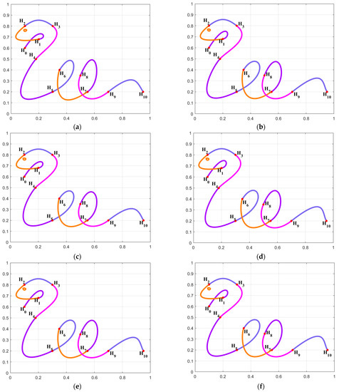
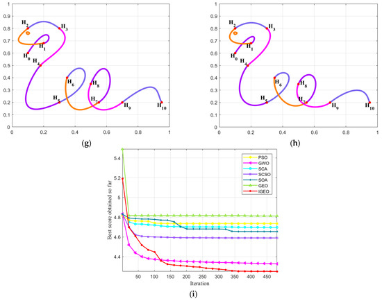
Figure 1.
Shape optimization of combined SGC-Ball interpolation curves with “snake” shapes. (a) ; (b) ; (c) ; (d) ; (e) ; (f) ; (g) ; (h) ; (i) curve energy variation chart.
The optimization curves obtained by solving the C1 smooth concatenated combined SGC-Ball interpolation curves using various optimization algorithms are shown in Figure 1b–h. It can be observed that the constructed “snake” interpolation curves consist of 10 SGC-Ball interpolation curves, with different colored curves representing different SGC-Ball interpolation curves, as well as the shape of the interpolation curves optimized by different algorithms is different, but the difference is not significant, which is caused by different parameter values. The energy convergence changes for all algorithms are drawn in Figure 1i. It is discovered that the IGEO-obtained energy convergence curves can swiftly converge to the least energy, demonstrating that IGEO is better to other comparison methods. Meanwhile, Table 1 provides the minimum energy and related shape parameter values of each algorithm for solving C1 smooth continuation “snake” interpolation curves. The results obtained are the average values of the results obtained by each algorithm after 30 independent runs. According to Table 1, the energy obtained by IGEO is the minimum, with a value of 69.6892, which means it has the smoothest curve shape. Compared with other algorithms, IGEO has the best performance, competitiveness, and superiority in solving the C1 smooth concatenation shape optimization model of combined SGC-Ball interpolation curves.

Table 1.
Results of each algorithm corresponding to Example 1.
Example 2.
The coordinates of the data points to be interpolated are given as follows:
By using the combined SGC-Ball interpolation curves to interpolate the given data points , the “cherry” shaped graph was designed, which satisfies the C2 smooth continuity splicing condition. The constructed “cherry” interpolation curves consist of 14 SGC-Ball interpolation curves, with different colored curves representing different SGC-Ball interpolation curves, and 43 shape parameters to be optimized.
Figure 2 displayed the experimental results of utilizing various algorithms to solve the established C2 continuous combined SGC-Ball interpolation curve optimization model. Among them, Figure 2a shows the combined SGC-Ball interpolation curves with free parameters. Using IGEO, PSO, GWO, SCA, MFO, COOT and standard GJO to solve the shape optimization model of the “cherry” interpolation curves, the smoothest curves obtained are shown in Figure 2b–h. The energy convergence curves obtained from various algorithms are shown in Figure 2i, which can intuitively reflect the better of IGEO in dealing with this question.
Figure 2.
Shape optimization of combined SGC-Ball interpolation curves with “cherry” shapes. (a) ; (b) ; (c) ; (d) ; (e) ; (f) ; (g) ; (h) ; (i) curve energy variation chart.
Table 2 displays the minimum energy values and corresponding parameters after 30 runs. Observing these data, it is evident that compared with other algorithms, IGEO obtained the smoothest curve, with an energy value of 90.9885. Through this numerical example, it is proven that IGEO achieves the best results in solving the established combined SGC-Ball interpolation curves, and can obtain curve shapes with ideal shapes.
Table 2.
Results of each algorithm corresponding to Example 2.
Example 3.
The coordinates of the data points to be interpolated are given as follows:
By using the combined SGC-Ball interpolation curves to interpolate data points , the optimized curve with the “rabbit” shape is designed. The constructed “rabbit” interpolation curves consist of 39 SGC-Ball curves, with different colored curves representing different SGC-Ball interpolation curves, and 118 parameters to be optimized.
Figure 3a shows the “rabbit” curve model with given parameters, using different optimization algorithms to optimize the combined SGC-Ball interpolation curves. Figure 3b–h depict the smooth curves obtained by seven optimization methods. From a visual perspective, it can be seen that the curves are optimized by IGEO is the smoothest, indicating that IGEO has certain advantage in solving the optimization model. Figure 3i describes the energy change convergence curves of all algorithms, and it is found that IGEO exhibits better convergence performance when solving shape optimization problems.
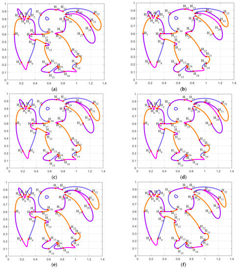
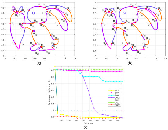
Figure 3.
Shape Optimization of combined SGC-Ball interpolation curves with “rabbit” shapes. (a) ; (b) ; (c) ; (d) ; (e) ; (f) ; (g) ; (h) ; (i) Curve energy variation chart.
Table A1 displays the experimental results of each technique to handle the curves’ shape optimization model, including optimal energy value and related parameter values, in order to more thoroughly examine the optimization impact of every technique to solve the curves shape model (see Appendix A). Compared with other competitive algorithm, IGEO achieved the minimum energy value of 358.0383, which is the combined SGC-Ball interpolation curves with the most ideal shape.
6. Conclusions and Future Works
This article first constructs the combined SGC-Ball interpolation curves and studies the conditions of the C1 and C2 smooth continuity of two adjacent SGC-Ball interpolation curves. The constructed combined SGC-Ball interpolation curves have global and local shape parameters, and have high flexibility in shape adjustment. Secondly, three improvements were integrated into the GEO: (1) The variety of the population increased after LF was introduced during the population’s initiation phase. (2) SCA enhances the development capacity and search scope of original GEO. (3) Using DE to escape local optima and increase the solution’s precision. The above three strategies work together on GEO, greatly boosting the effectiveness of GEO. Finally, depending on the minimum energy of the curve, the shape optimization models of combined SGC-Ball interpolation curves were established. The shape parameters in the models were optimized using the proposed IGEO to achieve the optimal interpolation curves. The solution results of IGEO were compared with other algorithms, and three numerical examples verified the superior performance of IGEO.
At present, the theoretical system and key technologies of generalized Ball interpolation curves and surfaces with multiple shape parameters are not yet perfect. This article only studies the construction, C1 and C2 smooth splicing, as well as shape optimization problems of combined SGC-Ball interpolation curves, further research is needed on the segmentation and extension algorithms of this curve in future work. In addition, we will consider extending the research technique of combined SGC-Ball interpolation curves to the CQGS-Ball surfaces in [77], and utilizing intelligent algorithms in [78] to investigate the shape optimization problem of the surfaces.
Author Contributions
Conceptualization, G.H.; methodology, J.Z., G.H., L.C. and X.J.; software, J.Z. and L.C.; validation, L.C. and G.H.; formal analysis, J.Z. and X.J.; investigation, J.Z., G.H., L.C. and X.J.; resources, X.J. and G.H.; writing—original draft, J.Z., G.H., L.C. and X.J.; writing—review and editing, J.Z., G.H., L.C. and X.J.; visualization, J.Z. and L.C.; supervision, X.J. and G.H.; project administration, X.J. and G.H.; funding acquisition, G.H. All authors have read and agreed to the published version of the manuscript.
Funding
This work is supported by the Project Supported by Natural Science Basic Research Plan in Shaanxi Province of China (No.2021JM320).
Data Availability Statement
All data generated or analyzed during this study were included in this published article.
Acknowledgments
The authors are very grateful to the reviewers for their insightful suggestions and comments, which helped us to improve the presentation and content of the paper.
Conflicts of Interest
The authors declare no conflict of interest.
Nomenclature
| Notations | Explanation |
| CAGD | Computer aided geometric design |
| CONSURF | A system name |
| CG-Ball | Cubic generalized Ball |
| CCG-Ball | Combined cubic generalized Ball |
| SGC-Ball | Shape-adjustable generalized cubic Ball |
| PSO | Particle swarm optimization |
| DE | Differential evolution |
| GSA | Gravitational search algorithm |
| NFL | No free lunch theorem |
| GA | Genetic algorithm |
| SA | Simulated annealing |
| GBO | Gradient-based optimizer |
| ASO | Atomic search optimization |
| LF | Lévy flight |
| ACO | Ant colony optimization |
| GWO | Grey wolf optimizer |
| HHO | Harris hawks optimization |
| SOA | Seagull optimization algorithm |
| CSA | Chameleon swarm algorithm |
| AHA | Artificial hummingbird algorithm |
| ARO | Artificial rabbits optimization |
| SCSO | Sand cat swarm optimization |
| TLBO | Teaching-learning-based optimization |
| GJO | Golden jackal optimization |
| GEO | Golden eagle optimizer |
| IGEO | Improved golden eagle optimizer |
| SCA | Sine cosine algorithm |
Appendix A
Table A1.
Results of each algorithm corresponding to Example 3.
Table A1.
Results of each algorithm corresponding to Example 3.
| Algorithms | Parameter | Shape Parameter Values | |
|---|---|---|---|
| WOA | 0.5436 | 362.4111 | |
| 2.954, 2.932, 2.926, 2.928, 2.934, 2.925, 2.931, 2.878, 2.761, 2.861, 2.897, 2.91, 2.911, 2.917, 2.935, 2.913, 2.934, 2.921, 2.909, 2.927, 2.906, 2.914, 2.929, 2.928, 2.943, 2.928, 2.935, 2.908, 2.907, 2.925, 2.935, 2.869, 2.916, 2.928, 2.924, 2.919, 2.923, 2.921, 2.912 | |||
| 2.153, 2.137, 2.267, 2.062, 2.296, 2.155, 2.145, 2.349, 2.252, 2.177, 2.257, 2.188, 2.099, 2.214, 2.325, 2.219, 2.209, 2.279, 2.218, 2.185, 2.116, 2.252, 2.148, 2.289, 2.132, 2.183, 2.15, 2.165, 1.847, 2.102, 2.16, 2.197, 2.104, 2.165, 2.276, 2.25, 2.097, 2.315, 2.207 | |||
| 2.932, 2.932, 2.961, 2.922, 2.961, 2.937, 2.935, 2.953, 2.882, 2.913, 2.914, 2.947, 2.922, 2.933, 2.846, 2.937, 2.928, 2.929, 2.955, 2.939, 2.954, 2.944, 2.942, 2.935, 2.936, 2.95, 2.959, 2.968, 2.935, 2.934, 2.96, 2.947, 2.949, 2.935, 2.934, 2.928, 2.925, 2.934, 2.907 | |||
| SCA | 0.003814 | 725.0963 | |
| 0.3545, −1.188, −0.3691, −0.5076, 0.2061, −0.2963, −0.1863, 0.1929, 0.01715, 0.1436, −0.2236, −0.09907, −0.6327, −0.1962, −0.133, 0.544, 0.615, −0.3826, −0.8297, −0.2927, −0.1665, 0.2791, −0.3062, −0.1759, 0.04228, 0.04547, −0.2596, 0.1204, 0.2308, 0.7154, −0.3409, 0.6497, −0.2007, 0.06538, −0.1902, 0.1042, −0.1695, −0.1979, 0.4829 | |||
| 1.449, 2.132, 2.016, 1.405, 2.2, 1.862, 2.183, 1.923, 1.326, 1.998, 1.933, 1.683, 2.04, 1.953, 1.74, 2.158, 1.513, 1.658, 1.541, 2.005, 1.982, 2.095, 1.886, 1.774, 1.512, 1.606, 2.456, 2.189, 2.44, 1.788, 1.379, 1.626, 1.496, 2.66, 1.821, 1.846, 1.365, 1.952, 1.514 | |||
| 0.4121, −0.4958, −0.3137, 0.5515, 0.2239, 0.6315, 0.1162, 0.623, −0.02511, −0.1388, −0.1904, 0.2453, 0.05011, −0.1406, −0.3857, −0.5536, 0.00983, 0.03625, −0.1328, 0.0107, 0.6325, 0.2954, −0.1675, 0.2039, 0.2612, 0.1163, 0.4011, 0.1793, 0.2139, −0.04972, 0.762, 0.3163, 0.06849, 0.3149, 0.1689, 0.08049, 0.1229, −0.6091, 0.3028 | |||
| SOA | 0.01122 | 605.7008 | |
| −0.4834, 0.09124, 0.3709, 0.0602, −0.3799, −0.565, 0.6734, 0.1475, −0.0678, 0.2025, −0.5324, −0.4233, 0.1613, −0.8813, −0.1016, 0.0625, −0.432, 0.6457, 0.2398, −0.4466, −0.522, −0.2366, 0.6574, 0.8444, 0.05558, −0.1118, −0.6338, −0.1005, 0.2253, −0.1902, 0.6508, 0.2474, 0.3863, −0.3265, 0.5572, 0.5963, 0.8713, −0.1275, 0.4026 | |||
| 1.546, 1.881, 2.154, 1.798, 1.807, 2.019, 1.5, 1.99, 1.415, 1.897, 1.704, 1.559, 1.548, 1.827, 2.255, 2.234, 2,1.582, 1.918, 2.151, 1.91, 2.649, 1.62, 1.921, 1.564, 2.483, 2.094, 1.894, 2.789, 1.677, 2.195, 1.678, 1.488, 1.915, 2.696, 2, 1.872, 1.837, 1.822 | |||
| 0.3878, 0.1218, 0.5233, 0.9948, 1.009, 0.4664, −0.2176, −0.6146, 0.9582, 0.6611, 0.807, −0.2097, −0.1613, 0.5906, −0.01125, −0.2685, −0.2075, −0.1658, 0.1493, 0.612, −0.0003401, 1.208, 0.2315, 0.5421, 0.3291, −0.1309, 0.4645, 0.457, 0.5299, −0.4613, −0.5515, 0.09413, −0.1733, 0.8304, −0.03633, 0.6071, −0.08072, 0.7613, 0.2763 | |||
| COOT | 0.01787 | 361.1240 | |
| 0.01405, 0.7826, −0.2576, 0.1128, −0.511, 0.3602, 0.4929, 0.3394, −0.0761, 0.08219, −0.01517, −0.3585, −0.189, 0.4331, 0.0848, 0.1457, 0.2874, 0.1497, −0.2239, 0.1698, 0.355, 0.06232, −0.1226, −0.2063, 0.00622, −0.2101, −0.0185, 0.4508, 0.3709, −0.4185, 0.4222, −0.1741, 0.06057, 0.1687, −0.03459, 0.8034, −0.0733, 0.06585, 0.01481 | |||
| 0.9079, 0.7436, 0.658, 0.5678, 0.9372, 0.7532, 0.6467, 0.7617, 0.7133, 0.8369, 1.067, 0.5985, 0.6435, 0.8064, 0.8836, 0.9601, 0.7917, 0.9659, 0.6913, 0.6973, 0.9516, 1.059, 0.7769, 0.7961, 1.144, 0.8362, 0.9826, 0.8728, 0.9639, 0.7841, 0.8724, 0.6207, 0.5075, 0.7312, 0.9063, 0.7258, 0.9735, 0.9084, 0.7264 | |||
| −0.2431, 0.3334, −0.3166, 0.4909, −0.8235, 0.1076, 0.2228, −0.4502, −0.4069, 0.4663, 0.2579, 0.3018, 0.3445, 0.6313, 0.534, 0.8747, −0.06324, 0.06046, 0.02741, 0.5181, 0.2365, 0.3449, 0.6841, 0.3307, −0.0763, 0.3352, −0.706, 0.2739, 0.209, −0.3769, 0.3075, 0.3207, 0.561, −0.0174, 0.4047, −0.08191, −0.1555, −0.3167, −0.3026 | |||
| SMA | 0.8568 | 399.8538 | |
| 2.141, 2.141, 2.141, 2.141, 2.141, 2.141, 2.141, 2.141, 2.141, 2.141, 2.141, 2.141, 2.141, 2.141, 2.141, 2.141, 2.141, 2.141, 2.141, 2.141, 2.141, 2.141, 2.141, 2.141, 2.141, 2.141, 2.141, 2.141, 2.141, 2.141, 2.141, 2.141, 2.141, 2.141, 2.141, 2.141, 2.141, 2.141, 2.141 | |||
| 3.427, 3.427, 3.427, 3.427, 3.427, 3.427, 3.427, 3.427, 3.427, 3.427, 3.427, 3.427, 3.427, 3.427, 3.427, 3.427, 3.427, 3.427, 3.427, 3.427, 3.427, 3.427, 3.427, 3.427, 3.427, 3.427, 3.427, 3.427, 3.427, 3.427, 3.427, 3.427, 3.427, 3.427, 3.427, 3.427, 3.427, 3.427, 3.427 | |||
| 2.141, 2.141, 2.141, 2.141, 2.141, 2.141, 2.141, 2.141, 2.141, 2.141, 2.141, 2.141, 2.141, 2.141, 2.141, 2.141, 2.141, 2.141, 2.141, 2.141, 2.141, 2.141, 2.141, 2.141, 2.141, 2.141, 2.141, 2.141, 2.141, 2.141, 2.141, 2.141, 2.141, 2.141, 2.141, 2.141, 2.141, 2.141, 2.141 | |||
| GEO | 0.001684 | 746.0022 | |
| 0.1044, −0.3334, −0.0137, −0.228, −0.7593, −0.0387, −0.4705, 0.3131, 0.00489, −0.4623, 0.3339, −0.127, −0.5072, −0.2334, 0.3881, −0.2313, 0.07534, 0.04545, 0.06941, −0.4636, −0.1516, −0.1319, 0.119, 0.4085, −0.0374, 0.5368, 0.07277, −0.1528, −0.0984, 0.3767, 0.2225, −0.1824, −0.04129, 0.3129, −0.06372, −0.2685, 0.102, −0.4658, −0.129 | |||
| 1.876, 2.126, 2.379, 1.741, 2.017, 1.991, 2.005, 2.051, 1.838, 2.051, 1.785, 2.29, 1.82, 2.148, 1.957, 2.03, 1.817, 2.036, 2.275, 1.827, 2.019, 2.376, 1.991, 2.131, 2.373, 2.237, 1.684, 2.38, 1.861, 2.072, 1.853, 2.024, 1.65, 2.259, 1.958, 2.217, 2.055, 1.607, 2.188 | |||
| 0.278, 0.2668, −0.209, 0.337, 0.121, −0.1014, −0.522, 0.228, −0.5336, 0.1272, −0.2752, −0.0881, −0.0024, 0.2046, −0.0467, 0.5206, 0.093, −0.0881, −0.126, 0.1704, 0.3037, −0.3562, 0.2501, −0.07322, 0.08496, −0.0584, −0.2581, 0.4829, 0.0478, −0.1881, −0.2741, −0.2411, −0.1592, −0.07102, 0.07086, 0.5762, 0.06904, −0.6406, 0.01202 | |||
| IGEO | 0.561 | 358.0384 | |
| 2.469, 2.299, 2.392, 2.229, 2.574, 2.455, 2.246, 2.117, 2.106, 2.236, 2.326, 2.194, 2.31, 2.284, 2.462, 2.053, 2.428, 2.451, 2.135, 2.506, 2.309, 2.176, 2.349, 2.332, 2.283, 2.298, 2.28, 2.56, 2.275, 2.231, 2.301, 2.248, 2.371, 1.919, 2.406, 2.028, 2.308, 2.187, 2.361 | |||
| 3.224, 3.358, 3.412, 3.236, 3.454, 3.272, 3.376, 3.387, 3.326, 3.356, 3.159, 3.404, 3.28, 3.335, 3.253, 3.342, 3.276, 3.2, 3.211, 3.339, 3.39, 3.232, 3.304, 3.153, 3.28, 3.202, 3.304, 3.407, 3.187, 3.314, 3.216, 3.353, 3.341, 3.355, 3.244, 3.257, 3.335, 3.24, 3.227 | |||
| 2.63, 2.351, 2.584, 2.338, 2.433, 2.184, 2.424, 2.266, 2.399, 2.164, 2.112, 2.312, 2.21, 2.347, 2.181, 2.223, 2.411, 2.321, 2.437, 2.294, 2.495, 2.411, 2.342, 2.126, 2.423, 2.445, 2.318, 2.408, 2.273, 2.519, 2.434, 2.543, 2.299, 2.227, 2.314, 2.389, 2.36, 2.314, 2.233 |
References
- Barnhill, R.E.; Riesenfeld, R.F. Computer Aided Geometric Design; Academic Press: New York, NY, USA, 1974. [Google Scholar]
- Farin, G. Curves and Surfaces for CAGD: A Practical Guide, 5th ed.; Academic Press: San Diego, CA, USA, 2002. [Google Scholar]
- Wang, G.J.; Liu, L.G. Approximation and Processing in Geometric Calculations; Science Press: Beijing, China, 2015. [Google Scholar]
- Kanetaki, Z.; Stergiou, C.; Troussas, C.; Sgoroupoulu, C. Development of an Innovative Learning Methodology Aiming to Optimise Learners’ Spatial Conception in an Online Mechanical CAD Module During COVID-19 Pandemic. In Novelties in Intelligent Digital Systems, Proceedings of the 1st International Conference (NIDS 2021), Athens, Greece, 30 September–1 October 2021; IOS Press: Amsterdam, The Netherlands, 2021; pp. 31–39. [Google Scholar]
- Zaranis, N.; Exarchakos, G.M. The Use of ICT and the Realistic Mathematics Education for Understanding Simple and Advanced Stereometry Shapes among University Students. In Research on e-Learning and ICT in Education; Mikropoulos, T., Ed.; Springer: Cham, Switzerland, 2018. [Google Scholar]
- Jaklič, G.; Kozak, J.; Vitrih, V.; Žagar, E. Lagrange geometric interpolation by rational spatial cubic Bézier curves. Comput. Aided Geom. Des. 2012, 29, 75–188. [Google Scholar] [CrossRef]
- Mao, A.H.; Luo, J.; Chen, J.; Li, G. A new fast normal-based interpolating subdivision scheme by cubic Bézier curves. Vis. Comput. 2016, 32, 1085–1095. [Google Scholar]
- Sarraga, R.F. G1 interpolation of generally unrestricted cubic Bézier curves. Comput. Aided Geom. Des. 1989, 4, 23–39. [Google Scholar] [CrossRef]
- Popiel, T.; Noakes, L. Bézier curves and C2 interpolation in Riemannian manifolds. J. Approx. Theory 2007, 148, 111–127. [Google Scholar] [CrossRef]
- Harada, K.; Nakamae, E. Application of the Bézier curve to data interpolation. Comput.-Aided Des. 1982, 14, 55–59. [Google Scholar] [CrossRef]
- Pal, S.; Biswas, P.K.; Abraham, A. Face Recognition Using Interpolated Bézier Curve Based Representation. In Proceedings of the International Conference on Information Technology: Coding & Computing, IEEE, Las Vegas, NV, USA, 5–7 April 2004. [Google Scholar]
- Wahab, A.F.; Zulkifly, M.I.E. Cubic Bézier curve interpolation by using intuitionistic fuzzy control point relation. AIP Conf. Proc. 2018, 1974, 020031. [Google Scholar]
- Lee, J.H.; Yang, S.N. Shape preserving and shape control with interpolating Bézier curves. J. Comput. Appl. Math. 1989, 28, 269–280. [Google Scholar] [CrossRef]
- Hu, G.; Zhu, X.N.; Wei, G.; Chang, C.T. An improved marine predators algorithm for shape optimization of developable Ball surfaces. Eng. Appl. Artif. Intell. 2021, 105, 104417. [Google Scholar] [CrossRef]
- Hu, G.; Li, M.; Wang, X.; Chang, C.T. An enhanced manta ray foraging optimization algorithm for shape optimization of complex CCG-Ball curves. Knowl.-Based Syst. 2022, 240, 108071. [Google Scholar] [CrossRef]
- Hu, G.; Li, M.; Zhong, J.Y. Combined cubic generalized ball surfaces: Construction and shape optimization using an enhanced JS algorithm. Adv. Eng. Softw. 2023, 176, 103404. [Google Scholar] [CrossRef]
- Jaklič, G.; Žagar, E. Curvature variation minimizing cubic Hermite interpolants. Appl. Math. Comput. 2011, 218, 3918–3924. [Google Scholar] [CrossRef]
- Lu, L.Z. A note on curvature variation minimizing cubic Hermite interpolants. Appl. Math. Comput. 2015, 259, 596–599. [Google Scholar] [CrossRef]
- Liu, C.; Li, J. Study on the optimal shape parameter of parametric curves based on PSO algorithm. J. Interdiscip. Math. 2016, 19, 321–333. [Google Scholar] [CrossRef]
- Hu, G.; Wu, J.L.; Li, H.N.; Hu, X. Shape optimization of generalized developable H-Bézier surfaces using adaptive cuckoo search algorithm. Adv. Eng. Softw. 2020, 149, 102889. [Google Scholar] [CrossRef]
- Hu, G.; Zhu, X.N.; Wang, X.; Wei, G. Multi-strategy boosted marine predators algorithm for optimizing approximate developable surface. Knowl.-Based Syst. 2022, 254, 109615. [Google Scholar] [CrossRef]
- Iman, A.; Aahb, C.; Ahg, D.; Gandomi, A.H.; Chu, X.; Chen, H. RUN beyond the metaphor: An efficient optimization algorithm based on runge kutta method. Expert Syst. Appl. 2021, 181, 115079. [Google Scholar]
- Houssein, E.H.; Saad, M.R.; Hashim, F.A.; Shaban, H.; Hassaballah, M. Lévy flight distribution: A new metaheuristic algorithm for solving engineering optimization problems. Eng. Appl. Artif. Intell. 2020, 94, 103731. [Google Scholar] [CrossRef]
- Houssein, E.H.; Helmy, E.D.; Oliva, D.; Elngar, A.A.; Shaban, H. A novel black widow optimization algorithm for multilevel thresholding image segmentation. Expert Syst. Appl. 2021, 167, 114159. [Google Scholar] [CrossRef]
- Wang, M.; Chen, H. Chaotic multi-swarm whale optimizer boosted support vector machine for medical diagnosis. Appl. Soft Comput. 2020, 88, 105946. [Google Scholar] [CrossRef]
- Neggaz, N.; Houssein, E.H.; Hussain, K. An efficient Henry gas solubility optimization for feature selection. Expert Syst. Appl. 2020, 152, 113364. [Google Scholar] [CrossRef]
- Hu, G.; Du, B.; Wang, X.F.; Wei, G. An enhanced black widow optimization algorithm for feature selection. Knowl.-Based Syst. 2022, 235, 107638. [Google Scholar] [CrossRef]
- Kennedy, J.; Eberhart, R. Particle swarm optimization. In Proceedings of the ICNN95—International Conference on Neural Networks, Perth, WA, Australia, 27 November–1 December 1995; Volume 4, pp. 1942–1948. [Google Scholar]
- Storn, R.; Price, K. Differential evolution-a simple and efficient heuristic for global optimization over continuous spaces. J. Glob. Optim. 1997, 11, 341–359. [Google Scholar] [CrossRef]
- Rashedi, E.; Nezamabadi-Pour, H.; Saryazdi, S. GSA: A gravitational search algorithm. Inf. Sci. 2009, 179, 2232–2248. [Google Scholar] [CrossRef]
- Wolpert, D.H.; Macready, W.G. No free lunch theorems for optimization. IEEE Trans. Evol. Comput. 1997, 1, 67–82. [Google Scholar] [CrossRef]
- Holland, J.H. Genetic algorithms. Sci. Am. 1992, 267, 66–72. [Google Scholar] [CrossRef]
- Kirkpatrick, S.; Gelatt, C.D.; Vecchi, M.P. Optimization by simulated annealing. Science 1983, 220, 671–680. [Google Scholar] [CrossRef]
- Ahmadianfar, I.; Bozorg-Haddad, O.; Chu, X. Gradient-based optimizer: A new Metaheuristic optimization algorithm. Inf. Sci. 2020, 540, 131–159. [Google Scholar] [CrossRef]
- Zhao, W.G.; Wang, L.Y.; Zhang, Z.X. A novel atom search optimization for dispersion coefficient estimation in groundwater. Future Gener. Comput. Syst. 2019, 91, 601–610. [Google Scholar] [CrossRef]
- Dorigo, M.; Caro, G.D. Ant colony optimization: A new meta-heuristic. In Proceedings of the 1999 Congress on Evolutionary Computation, Washington, DC, USA, 6–9 July 1999; Volume 2, pp. 1470–1477. [Google Scholar]
- Mirjalili, S.; Mirjalili, S.M.; Lewis, A. Grey wolf optimizer. Adv. Eng. Softw. 2014, 69, 46–61. [Google Scholar] [CrossRef]
- Heidari, A.A.; Mirjalili, S.; Faris, H.; Aljarah, I.; Mafarja, M.; Chen, H. Harris hawks optimization: Algorithm and applications. Future Gener. Comput. Syst. 2019, 97, 849–872. [Google Scholar] [CrossRef]
- Dhiman, G.; Kumar, V. Seagull optimization algorithm: Theory and its applications for large-scale industrial engineering problems. Knowl.-Based Syst. 2019, 165, 169–196. [Google Scholar] [CrossRef]
- Braik, M.S. Chameleon Swarm Algorithm: A bio-inspired optimizer for solving engineering design problems. Expert Syst. Appl. 2021, 174, 114685. [Google Scholar] [CrossRef]
- Hu, G.; Yang, R.; Qin, X.Q.; Wei, G. MCSA: Multi-strategy boosted chameleon-inspired optimization algorithm for engineering applications. Comput. Methods Appl. Mech. Eng. 2023, 403, 115676. [Google Scholar] [CrossRef]
- Zhao, W.G.; Wang, L.Y.; Mirjalili, S. Artificial hummingbird algorithm: A new bio-inspired optimizer with its engineering applications. Comput. Methods Appl. Mech. Eng. 2022, 388, 114194. [Google Scholar] [CrossRef]
- Wang, L.Y.; Cao, Q.J.; Zhang, Z.X. Artificial rabbits optimization: A new bio-inspired meta-heuristic algorithm for solving engineering optimization problems. Eng. Appl. Artif. Intell. 2022, 114, 105082. [Google Scholar] [CrossRef]
- Seyyedabbasi, A.; Kiani, F. Sand Cat swarm optimization: A nature-inspired algorithm to solve global optimization problems. Eng. Comput. 2022, 39, 2627–2651. [Google Scholar] [CrossRef]
- Rao, R.V.; Savsani, V.J.; Vakharia, D.P. Teaching-Learning-Based Optimization: An optimization method for continuous non-linear large scale problems. Inf. Sci. 2012, 183, 1–15. [Google Scholar] [CrossRef]
- Chopra, N.; Ansari, M.M. Golden jackal optimization: A novel nature-inspired optimizer for engineering applications. Expert Syst. Appl. 2022, 198, 116924. [Google Scholar] [CrossRef]
- Hu, G.; Zhong, J.; Wei, G.; Chang, C.-T. DTCSMO: An efficient hybrid starling murmuration optimizer for engineering applications. Comput. Methods Appl. Mech. Engrg. 2023, 405, 115878. [Google Scholar] [CrossRef]
- Hu, G.; Chen, L.X.; Wang, X.P.; Wei, G. Differential Evolution-Boosted Sine Cosine Golden Eagle Optimizer with Lévy Flight. J. Bionic Engineering. 2022, 19, 1850–1885. [Google Scholar]
- Ball, A.A. CONSURF: Part 1: Introduction to the conic lofting title. Comput.-Aided Des. 1974, 6, 243–249. [Google Scholar] [CrossRef]
- Ball, A.A. CONSURF: Part 2: Description of the algorithms. Comput.-Aided Des. 1975, 7, 237–242. [Google Scholar] [CrossRef]
- Ball, A.A. CONSURF: Part 3: How the program is used. Comput.-Aided Des. 1977, 9, 9–12. [Google Scholar] [CrossRef]
- Wang, G.J. High order Ball curves and their applications. J. Appl. Math. 1987, 2, 126–140. [Google Scholar]
- Said, H.B. Generalized Ball curve and its recursive algorithm. ACM Trans. Graph. 1989, 8, 360–371. [Google Scholar] [CrossRef]
- Hu, S.M.; Wang, G.Z.; Jin, T.G. Properties of two types of generalized Ball curves. CAD Comput. Aided Des. 1996, 28, 125–133. [Google Scholar] [CrossRef]
- Othnan, W.; Goldman, R.N. The dual basis funetions for the genearlized Ball basis of odd degere. CAGD 1997, 14, 571–582. [Google Scholar]
- Xi, M.C. Dual basis of Ball basis function and its application. Comput. Math. 1997, 19, 147–153. [Google Scholar]
- Ding, D.Y.; Li, M. The properties and applications of generalized Ball curves. J. Appl. Math. 2000, 23, 123–131. [Google Scholar]
- Wu, H.Y. Two new types of generalized Ball curves. J. Appl. Math. 2000, 23, 196–205. [Google Scholar]
- Wang, C.W. Extension of Cubic Ball Curve. J. Eng. Graph. 2008, 29, 77–81. [Google Scholar]
- Wang, C.W. Extension of the Fourth Degree Wang Ball Curve. J. Eng. Graph. 2009, 30, 80–84. [Google Scholar]
- Xiong, J.; Guo, Q.W. Generalized Said Ball curve. Numer. Calc. Comput. Appl. 2012, 33, 32–40. [Google Scholar]
- Xiong, J.; Guo, Q.W. Generalized Wang Ball Curve. Numer. Calc. Comput. Appl. 2013, 34, 187–195. [Google Scholar]
- Man, J.J.; Hu, S.M.; Yong, J.H. Reduced approximation of Bézier curves. J. Tsinghua Univ. 2000, 40, 117–120. [Google Scholar]
- Jaafar, W.; Piah, A.; Abbas, M. Shape preserving rational cubic Ball interpolation for positive data. In Proceedings of the National Symposium on Mathematical Sciences 2013 (SKSM21), Penang, Malaysia, 6–8 November 2013; American Institute of Physics: College Park, MD, USA, 2014; pp. 325–330. [Google Scholar]
- Hasan, Z.A.; Piah, A.R.M.; Yahya, Z.R. Monotonicity preserving C1 rational cubic Ball interpolation. In Proceedings of the 21st National Symposium on Mathematical Sciences (SKSM21), Penang, Malaysia, 6–8 November 2013; American Institute of Physics: College Park, MD, USA, 2014; pp. 34–39. [Google Scholar]
- Jamil, S.J.; Piah, A.R.M. C2 positivity-preserving rational cubic Ball interpolation. In Proceedings of the National Symposium on Mathematical Sciences 2013 (SKSM21), Penang, Malaysia, 6–8 November 2013; American Institute of Physics: College Park, MD, USA, 2014; pp. 337–342. [Google Scholar]
- Karim, S.A.A.; Hasan, M.K.; Sulaiman, J. Convexity preserving using GC1 cubic Ball interpolation. Appl. Math. Sci. 2014, 8, 2087–2100. [Google Scholar]
- Karim, S.A.A. Positivity preserving interpolation by using rational cubic Ball spline. J. Teknol. 2016, 78, 141–148. [Google Scholar]
- Mohammadi-Balani, A.; Nayeri, M.D.; Azar, A.; Taghizadeh-Yazdi, M. Golden eagle optimizer: A nature-inspired metaheuristic algorithm. Comput. Ind. Eng. 2021, 152, 107050. [Google Scholar] [CrossRef]
- Pan, J.S.; Lv, J.X.; Yan, L.J.; Weng, S.W.; Chu, S.C.; Xue, J.K. Golden eagle optimizer with double learning strategies for 3D path planning of UAV in power inspection. Math. Comput. Simul. 2021, 193, 509–532. [Google Scholar] [CrossRef]
- Zarkandi, S. Dynamic modeling and power optimization of a 4R P SP+PS parallel flight simulator machine. Robotica 2022, 40, 646–671. [Google Scholar] [CrossRef]
- Chandran, J.; Karthick, R.; Rajagopal, R.; Meenalochini, P. Dual-Channel Capsule Generative Adversarial Network Optimized with Golden Eagle Optimization for Pediatric Bone Age Assessment from Hand X-Ray Image. Int. J. Pattern Recognit. Artif. Intell. 2023, 37, 2354001. [Google Scholar] [CrossRef]
- Kumar, N.; Balasubramanian, C. Hybrid Gradient Descent Golden Eagle Optimization (HGDGEO) Algorithm-Based Efficient Heterogeneous Resource Scheduling for Big Data Processing on Clouds. Wirel. Pers. Commun. 2023, 129, 1175–1195. [Google Scholar] [CrossRef]
- Boriratrit, S.; Fuangfoo, P.; Srithapon, C.; Chatthaworn, R. Adaptive meta-learning extreme learning machine with golden eagle optimization and logistic map for forecasting the incomplete data of solar irradiance. Energy AI 2023, 13, 100243. [Google Scholar] [CrossRef]
- Charin, C.; Ishak, D.; Zainuri, M.; Ismail, B.; Jamil, M.K.M. A hybrid of bio-inspired algorithm based on Levy flight and particle swarm optimizations for photovoltaic system under partial shading conditions. Sol. Energy 2021, 217, 1–14. [Google Scholar] [CrossRef]
- Mirjalili, S. SCA: A Sine Cosine Algorithm for Solving Optimization Problems. Knowl.-Based Syst. 2016, 96, 120–133. [Google Scholar] [CrossRef]
- Zheng, J.; Ji, X.; Ma, Z.; Hu, G. Construction of Local-Shape-Controlled Quartic Generalized Said-Ball Model. Mathematics 2023, 11, 2369. [Google Scholar] [CrossRef]
- Hu, G.; Wang, J.; Li, M.; Hussien, A.G.; Abbas, M. EJS: Multi-strategy enhanced jellyfish search algorithm for engineering applications. Mathematics 2023, 11, 851. [Google Scholar] [CrossRef]


Disclaimer/Publisher’s Note: The statements, opinions and data contained in all publications are solely those of the individual author(s) and contributor(s) and not of MDPI and/or the editor(s). MDPI and/or the editor(s) disclaim responsibility for any injury to people or property resulting from any ideas, methods, instructions or products referred to in the content. |
© 2023 by the authors. Licensee MDPI, Basel, Switzerland. This article is an open access article distributed under the terms and conditions of the Creative Commons Attribution (CC BY) license (https://creativecommons.org/licenses/by/4.0/).