A Novel Two-Step Inertial Viscosity Algorithm for Bilevel Optimization Problems Applied to Image Recovery

Abstract

This paper introduces a novel two-step inertial algorithm for locating a common fixed point of a countable family of nonexpansive mappings. We establish strong convergence properties of the proposed method under mild conditions and employ it to solve convex bilevel optimization problems. The method is further applied to the image recovery problem. Our numerical experiments show that the proposed method achieves faster convergence than other related methods in the literature.

1. Introduction

Bilevel optimization has received significant attention in recent years, having arisen as a powerful tool for many machine learning applications such as hyperparameter optimization [1,2], signal processing [3,4], and reinforcement learning [5]. It is defined as a mathematical program in which an optimization problem contains another optimization problem as a constraint. In this paper, we consider the bilevel optimization problem in which the following minima are sought:

$$\begin{array}{c}\hfill \underset{x\in S_{*}}{min}\omega \left(x\right),\end{array}$$

(1)

where $\omega :{\mathbb{R}}^n\to \mathbb{R}$ is assumed to be strongly convex and differentiable, while $S_{*}$ is a nonempty set of inner level optimizers satisfying

$$\begin{array}{c}\hfill \underset{x\in {\mathbb{R}}^n}{min}\{{\psi }_1\left(x\right)+{\psi }_2\left(x\right)\},\end{array}$$

(2)

where ${\psi }_1:{\mathbb{R}}^n\to \mathbb{R}$ is a differentiable and convex function such that $\nabla {\psi }_1$ is L-Lipschitz continuous and ${\psi }_2:{\mathbb{R}}^n\to \mathbb{R}\cup \{\infty \}$ is a convex, proper, and lower semi-continuous function. We let $\mathsf{\Lambda }$ be the solution set of (1).

Observe that this bilevel optimization model contains the inner level minimization problem (2) as a constraint to the outer level optimization problem (1). It is a well-known form (1) that

$$x^{*}\in \mathsf{\Lambda }\mathrm{if}\mathrm{and}\mathrm{only}\mathrm{if}⟨\nabla \omega \left(x^{*}\right),x-x^{*}⟩\ge 0\mathrm{for}\mathrm{all}x\in S_{*}.$$

Many researchers have proposed algorithms for solving problem (2); see [6,7,8,9,10]. The basic algorithm is the proximal forward–backward technique, or proximal gradient method, defined by the iterative equation

$$\begin{array}{c}\hfill x_{n+1}=pro{x}_{{\alpha }_n{\psi }_2}(I-{\alpha }_n\nabla {\psi }_1)\left(x_n\right),n\in \mathbb{N},\end{array}$$

(3)

where ${\alpha }_n>0$ is the step-size, $pro{x}_{{\psi }_2}$ is the proximity operator of ${\psi }_2$, and $\nabla {\psi }_1$ is the gradient of ${\psi }_1$ [6,11]. Equation (3) is referred to in the literature as the forward–backward splitting algorithm (FBSA). The FBSA can be used to solve the inner level optimization problem if ${\psi }_1$ is L-Lipschitz continuous [7].

The proximal gradient method can also be viewed as a fixed-point algorithm, where the iterated mapping is given by

$$\begin{array}{c}\hfill T:=pro{g}_{\alpha {\psi }_2}(I-\alpha \nabla {\psi }_1)\end{array}$$

(4)

and is called the forward–backward mapping [12]. The forward–backward mapping, T, is nonexpansive if $0<\alpha <2/L$, where L is a Lipschitz constant of $\nabla {\psi }_1$ and, in that case, $Fix\left(T\right)=argmin\{{\psi }_1\left(x\right)+{\psi }_2\left(x\right)\}$. It is noted that implementation of the forward–backward operator can be simplified by first changing the inner level optimization problem into a zero-point problem of the sum of two monotone operators, and then, after analysis, translating back into the fixed-point problem. Exemplifying the fixed-point approach, Sabach et al. [13] proposed the bilevel gradient sequential averaging method (BiG-SAM) for solving problems (1) and (2). The iterative process can be defined as

$$\begin{array}{c}\hfill \left\{\begin{array}{c}{u}_n=pro{x}_{cg}(x_{n-1}-c\nabla f\left(x_{n-1}\right)),\hfill \\ v_n=x_{n-1}-\lambda \nabla \omega \left(x_{n-1}\right),\hfill \\ x_{n+1}={\gamma }_n{v}_n+(1-{\gamma }_n)u_n,n\ge 1\hfill \end{array}\right.\end{array}$$

(5)

where $c\in (0,\frac{2}{L_f}),$$\lambda \in (0,\frac{2}{L_{\omega }+\sigma })$, $\omega$ is strongly convex with parameter $\sigma ,$ and where $L_f$ and $L_{\omega }$ are Lipschitz constants for the gradients of f and $\omega$. The authors analyzed the convergence behavior of BiG-SAM using an existing fixed-point algorithm and discussed its rate of convergence.

In optimization problems like those presented above, mathematicians frequently employ a technique known as inertial-type extrapolation [14,15] to accelerate the convergence of the iterative equations. This approach involves utilizing a term ${\theta }_n(x_n-x_{n-1})$, where ${\theta }_n$ denotes an inertial parameter, to govern the momentum $x_n-x_{n-1}$. One such algorithm that has enjoyed immense popularity was developed by Nesterov [14]. He used an inertial or extrapolation technique to solve convex optimization problems of the form of (2), where $F:={\psi }_1+{\psi }_2$ is a convex, smooth function. Nesterov’s algorithm takes the following form:

$$\begin{array}{c}\hfill \left\{\begin{array}{c}{z}_n=x_n+{\theta }_n(x_n-x_{n-1}),\hfill \\ x_{n+1}=z_n+c\nabla F\left(z_n\right),n\in \mathbb{N},\hfill \end{array}\right.\end{array}$$

(6)

where the inertial parameter ${\theta }_n\in (0,1)$ for all n and $c>0$ is the step size depending on the Lipschitz continuity modulus of $\nabla F$. Nesterov proved that Equation (6) has a faster convergence rate than the general gradient algorithm by selecting $\left\{{\theta }_n\right\}$ such that ${sup}_n{\theta }_n=1$. Similarly, in 2009, Beck et al. [16] introduced the fast iterative shrinkage-thresholding algorithm (FISTA) for solving linear inverse problems. Their result combined the proximity algorithm with the inertial technique, again resulting in the algorithm’s convergence rate being considerably accelerated.

In 2019, Shehu et al. [17] presented an inertial forward–backward algorithm, called the inertial bilevel gradient sequential averaging method (iBiG-SAM) for solving problems (1) and (2). Their method was subsequently improved by Sabach et al. [13], using the following iterative algorithm:

$$\begin{array}{c}\hfill \left\{\begin{array}{c}{s}_n=x_n+{\theta }_n(x_n-x_{n-1}),\hfill \\ u_n=pro{x}_{cg}(I-c\nabla f)\left(s_n\right),\hfill \\ v_n=s_n-\lambda \nabla \omega \left(s_n\right),\hfill \\ x_{n+1}={\gamma }_n{v}_n+(1-{\gamma }_n)u_n,n\ge 1.\hfill \end{array}\right.\end{array}$$

(7)

The authors transformed the bilevel optimization problem into a fixed-point problem for a nonexpansive mapping in an infinite dimensional Hilbert space and then proved strong convergence.

As the above suggests, research on fixed-point problems for nonexpansive mappings has become crucial for developing optimization methods. The Mann iterative process is a well-known method for approximating fixed points of nonexpansive mappings on Hilbert spaces. However, Mann’s process provides only weak convergence. Many authors have demonstrated fixed-point problems exhibiting strong convergence for nonexpansive mappings on Hilbert spaces using the viscosity approximation method, expressed by the equation

$$\begin{array}{c}\hfill x_{n+1}={\beta }_{n}S\left(x_n\right)+(1-{\beta }_n)T{x}_n,n\ge 1,\end{array}$$

(8)

where $\left\{{\beta }_n\right\}\in (0,1)$, S is a contraction on Hilbert spaces H and $x_1\in H$; see [18,19].

In 2009, Takahashi [20] modified the viscosity approximation method, selecting a particular fixed point of the nonexpansive self-mapping of Moudafi [18]. The iterative process is given by

$$\begin{array}{c}\hfill x_{n+1}={\beta }_{n}S\left(x_n\right)+(1-{\beta }_n)T_n{x}_n,n\ge 1,\end{array}$$

(9)

where $\left\{{\beta }_n\right\}\in (0,1)$, S is a contraction of C into itself, $\left\{T_n\right\}$ is a countable family of nonexpansive of C into itself, C is subset of a Banach space, and $x_1\in C$. Takahashi proved the strong convergence of (9) to a common fixed point of $T_n$.

Jailoka et al. [21] introduced a fast viscosity forward–backward algorithm (FVFBA) with the inertial technique for finding a common fixed point of a countable family of nonexpansive mappings. They proved a strong convergence result and applied it to solving a convex minimization problem of the sum of two convex functions. The  iterative process can be formulated by

$$\begin{array}{c}\hfill \left\{\begin{array}{c}{u}_n=x_n+{\theta }_n(x_n-x_{n-1}),\hfill \\ v_n=(1-{\alpha }_n)T_n{u}_n+{\alpha }_{n}S\left(u_n\right),\hfill \\ x_{n+1}=(1-{\beta }_n)T_n{u}_n+{\beta }_n{T}_n{v}_n,n\ge 1,\hfill \end{array}\right.\end{array}$$

(10)

where $\left\{{\alpha }_n\right\}, \left\{{\beta }_n\right\}\in (0,1)$, S is a contraction on Hilbert spaces H and $x_1\in H$.

Recently, Janngam et al. [22] presented an inertial viscosity modified SP algorithm (IVMSPA). The authors proved a strong convergence of their algorithm and applied it to solving the convex bilevel optimization problems (problems 1 and 2). Their algorithm was given by

$$\begin{array}{c}\begin{array}{c}{y}_n=x_n+{\theta }_n(x_n-x_{n-1}),\hfill \\ z_n=(1-{\alpha }_n)y_n+{\alpha }_{n}S\left(y_n\right),\hfill \\ w_n=(1-{\beta }_n)z_n+{\beta }_n{T}_n{z}_n,\hfill \\ x_{n+1}=(1-{\gamma }_n)w_n+{\gamma }_n{T}_n{w}_n,n\ge 1,\hfill \end{array}\end{array}$$

(11)

where $\left\{{\alpha }_n\right\}$, $\left\{{\beta }_n\right\}$, $\left\{{\gamma }_n\right\}\in (0,1)$, S is contraction mapping on Hilbert spaces H and $x_1\in H$.

The above authors all employ a single inertial parameter to accelerate the convergence of their algorithms. However, it has been noted that the incorporation of two inertial parameters enhances motion modeling, improves stability and robustness, increases redundancy and fault tolerance, expands the range of applications, and offers flexibility and adaptability in algorithm design. In [23], it was illustrated through an example that the one-step inertial extrapolation, expressed as $w_n=x_n+{\theta }_n(x_n-x_{n-1})$ with ${\theta }_n\in [0,1)$, may not produce acceleration. Additionally, Ref. [24] mentioned that incorporating more than two points, such as $x_n$ and $x_{n-1}$, in the inertial process could lead to acceleration. For instance, consider the following two-step inertial extrapolation:

$$\begin{array}{c}\hfill y_n=x_n+\theta (x_n-x_{n-1})+\delta (x_{n-1}-x_{n-2})\end{array}$$

(12)

where $\theta >0$ and $\delta <0$ can provide acceleration. The limitations of employing one-step inertial acceleration in the alternating direction method of multipliers (ADMM) were dissused in [25], which led to the proposal of adaptive acceleration as an alternative solution. In addition, Polyak [26] discussed the potential for multi-step inertial methods to enhance the speed of optimization techniques despite the absence of established convergence or rate results in [26]. Recent research conducted in [27] has further explored and examined various aspects of multi-step inertial methods.

Based on the information provided above, our aim in this paper is to solve the convex bilevel optimization problem by introducing a new accelerated viscosity algorithm with the two-point inertial technique, which we then apply to image recovery. The remainder of the paper is organized as follows. In Section 2, we recall some basic definitions and results that are crucial in the paper. The proposed algorithm and the analysis of its convergence are presented in Section 3. The performance of deblurring images using our algorithm is analyzed and illustrated in Section 4. Finally, we give conclusions and discuss directions for future work in Section 5.

2. Preliminaries

In this section, we present some preliminary material that will be needed for the main theorems.

Let C be a nonempty subset of a real Hilbert space H with norm $\parallel ·\parallel$, $\mathbb{R}$ denote the set of real numbers, ${\mathbb{R}}_{+}$ denote the non-negative real numbers, ${\mathbb{R}}_{>0}$ denote the positive real numbers, $\mathbb{N}$ denote the set of positive integers, and let I denote the identity mapping on H.

Definition 1.

The mapping $T:C\to C$ is said to be L-Lipschitz with $L\ge 0$, if 

$$\parallel Tu-Tv\parallel \le L\parallel u-v\parallel$$

for all $u,v\in C$. Furthermore, if $L\in [0,1)$ then T is called a contraction mapping, and it is nonexpansive if $L=1$.

When $\left\{x_n\right\}$ is a sequence in C, we denote the strong convergence of $x_n$ to $x\in C$ by $x_n\to x$, and $Fix\left(T\right)$ will symbolize the set of all fixed points of T.

Let $T:C\to C$ be a nonexpansive mapping and $\left\{T_n\right\}$ be a family of nonexpansive mappings of C into itself such that $\varnothing \ne Fix\left(T\right)\subset \mathsf{\Gamma }:={\bigcap }_{n=1}^{\infty }Fix\left(T_n\right)$. The sequence $\left\{T_n\right\}$ is said to satisfy the NST-condition (I) with T [28], if for each bounded sequence $\left\{x_n\right\}\subset C$,

$$\underset{n\to \infty }{lim}\parallel x_n-T_n{x}_n\parallel =0\mathrm{implies}\underset{n\to \infty }{lim}\parallel x_n-T{x}_n\parallel =0.$$

The following condition is an essential condition for proving our convergence theorem.

Definition 2

([29,30]). A sequence $\left\{T_n\right\}$ with ${\bigcap }_{n=1}^{\infty }Fix\left(T_n\right)\ne \varnothing$ is said to satisfy the condition (Z) if for every bounded sequence $\left\{u_n\right\}$ in C such that

$$\begin{array}{c}\hfill \underset{n\to \infty }{lim}\parallel u_n-T_n{u}_n\parallel =0,\end{array}$$

then, every weak cluster point of $\left\{u_n\right\}$ belongs to ${\bigcap }_{n=1}^{\infty }Fix\left(T_n\right)$.

Recall that for a nonempty closed convex subset C of H, the metric projection on C is a mapping $P_C:H\to C$, defined by

$$\begin{array}{c}\hfill P_{C}x=argmin\{\parallel x-y\parallel :y\in C\}\end{array}$$

for all $x\in H$. Note that $v=P_{C}x$ if and only if $⟨x-v,y-v⟩\le 0$ for all $y\in C$.

The definition and properties of a proximity operator are presented below.

Definition 3

([31,32]). Let $g:H\to \mathbb{R}\cup \{\infty \}$ be a function that is convex, proper, and lower semi-continuous. The function $pro{x}_g$, known as the proximity operator of g, is defined as follows:

$$\begin{array}{c}\hfill pro{x}_g\left(x\right):=\underset{y\in H}{min}\left(g\left(y\right)+\frac{1}{2}{\parallel x-y\parallel }^2\right).\end{array}$$

Alternatively, it can be expressed as:

$$pro{x}_g={(I+\partial g)}^{-1},$$

where $\partial g$ represents the subdifferential of g defined by:

$$\partial g\left(x\right):=\{v\in H:g(x)+⟨v,u-x⟩\le g(u)\mathit{for}\mathit{all}u\in H\}$$

for any $x\in H$. Additionally, for $\rho >0$, we know that $pro{x}_{\rho g}$ is firmly nonexpansive and

$$Fix\left(pro{x}_{\rho g}\right)=Argmin\left(g\right):=\{v\in H:g\left(v\right)\le g\left(u\right)\mathit{for}\mathit{all}u\in H\},$$

where $Fix\left(pro{x}_{\rho g}\right)$ is the set of fixed points of $pro{x}_{\rho g}$.

The following lemmas will be used for proving the convergence of our proposed algorithm.

Lemma 1

([33]). Let $\mathfrak{g}:H\to \mathbb{R}\cup \{\infty \}$ be a convex, proper, and lower semi-continuous function and let $\mathfrak{f}:H\to \mathbb{R}$ be a differentiable and convex function such that $\nabla \mathfrak{f}$ is L-Lipschitz continuous. Let

$$T_n:=pro{x}_{{\rho }_n\mathfrak{g}}(I-{\rho }_n\nabla \mathfrak{f})\mathit{and}T:=pro{x}_{\rho \mathfrak{g}}(I-\rho \nabla \mathfrak{f}),$$

where ${\rho }_n,\rho \in (0,2/L)$ with ${\rho }_n\to \rho$ as $n\to \infty$. Then $\left\{T_n\right\}$ satisfies the NST-condition (I) with T.

Lemma 2

([34]). Let $x_1,x_2\in H$ and $t\in [0,1]$. Then, the following properties are true:

(i) 

${\parallel x_1\pm x_2\parallel }^2={\parallel x_1\parallel }^2\pm 2⟨x_1,x_2⟩+{\parallel x_2\parallel }^2$;

(ii) 

${\parallel x_1+x_2\parallel }^2\le {\parallel x_1\parallel }^2+2⟨x_2,x_1+x_2⟩$;

(iii) 

${\parallel t{x}_1+(1-t)x_2\parallel }^2={t\parallel x_1\parallel }^2+(1-t){\parallel x_2\parallel }^2-t(1-t){\parallel x_1-x_2\parallel }^2$.

Lemma 3

([35]). Let $\left\{a_n\right\}$, $\left\{b_n\right\}\subset {\mathbb{R}}_{+}$ and $\left\{t_n\right\}\subset (0,1)$ such that ${\sum }_{n=1}^{\infty }{t}_n=\infty$. Assume that

$$a_{n+1}\le (1-t_n)a_n+t_n{b}_n$$

for all $n\in \mathbb{N}$. If ${lim\; sup}_{i\to \infty }{b}_{n_i}\le 0$ for every subsequence $\left\{a_{n_i}\right\}$ of $\left\{a_n\right\}$ satisfying

$$\underset{i\to \infty }{lim\; inf}(a_{n_i+1}-a_{n_i})\ge 0,$$

then ${lim}_{n\to \infty }{a}_n=0$.

3. Main Results

Throughout this section, we let C be closed convex with $\varnothing \ne C\subset H$ and a mapping $F:C\to C$ be a k-contraction where $0<k<1$. Let $\left\{T_n\right\}$ is a family of nonexpansive mappings of C into itself satisfying the condition (Z) such that $\mathsf{\Gamma }:={\bigcap }_{n=1}^{\infty }Fix\left(T_n\right)\ne \varnothing$.

For the first of our main results, we draw upon the ideas of Jailoka et al. [21] and Liang [24] and introduce a modified two-step inertial viscosity algorithm (MTIVA) for finding a common fixed point of a family of nonexpansive mappings $\left\{T_n\right\}$, as follows:

In Theorem 1, we show that Algorithm 1 converges strongly.

Algorithm 1 Modified Two-Step Inertial Viscosity Algorithm (MTIVA)

Initialization: Let $\left\{{\beta }_n\right\}$, $\left\{{\gamma }_n\right\}\subset [0,1]$, $\left\{{\tau }_n\right\}\subset {\mathbb{R}}_{+}$ and let $\left\{{\mu }_n\right\}$, $\left\{{\rho }_n\right\}\subset {\mathbb{R}}_{>0}$ be bounded sequences. Take $x_{-1}, x_0, x_1\in H$ arbitrarily. For $n\in \mathbb{N}$.

Step 1. Compute the inertial step: $$\begin{array}{c}\hfill {\vartheta }_n=\left\{\begin{array}{c}min\left\{{\mu }_n,\frac{{\tau }_n}{\parallel x_n-x_{n-1}\parallel }\right\}\mathrm{if}{x}_n\ne x_{n-1},\hfill \\ {\mu }_n\mathrm{otherwise},\hfill \end{array}\right.\end{array}$$ (13) and $$\begin{array}{c}\hfill {\delta }_n=\left\{\begin{array}{c}max\left\{-{\rho }_n,\frac{-{\tau }_n}{\parallel x_{n-1}-x_{n-2}\parallel }\right\}\mathrm{if}{x}_{n-1}\ne x_{n-2},\hfill \\ -{\rho }_n\mathrm{otherwise},\hfill \end{array}\right.\end{array}$$ (14) $$\begin{array}{c}\hfill w_n=x_n+{\vartheta }_n(x_n-x_{n-1})+{\delta }_n(x_{n-1}-x_{n-2}).\end{array}$$ (15)

Step 2. Compute the viscosity step: $$\begin{array}{c}\hfill z_n=(1-{\gamma }_n)T_n{w}_n+{\gamma }_{n}F\left(w_n\right).\end{array}$$ (16)

Step 3. Compute $x_{n+1}$: $$\begin{array}{c}\hfill x_{n+1}=(1-{\beta }_n)T_n{w}_n+{\beta }_n{T}_n{z}_n.\end{array}$$ (17)

Theorem 1.

Let a sequence $\left\{x_n\right\}$ be generated by Algorithm 1. Suppose the conditions (C1–C3) hold for the sequences $\left\{{\tau }_n\right\}$, $\left\{{\gamma }_n\right\}$, and $\left\{{\beta }_n\right\}$. Then, $x_n\to \breve{p}\in \mathsf{\Gamma }$, where $\breve{p}=P_{\mathsf{\Gamma }}F\left(\breve{p}\right)$.

(C1) 

${lim}_{n\to \infty }\frac{{\tau }_n}{{\gamma }_n}=0;$

(C2) 

$0<{ϵ}_1\le {\beta }_n\le {ϵ}_2<1$ for some ${ϵ}_1$, ${ϵ}_2\in \mathbb{R};$

(C3) 

$0<{\gamma }_n<1$, ${lim}_{n\to \infty }{\gamma }_n=0$ and ${\sum }_{n=1}^{\infty }{\gamma }_n=\infty$.

Proof. 

Let $\breve{p}=P_{\mathsf{\Gamma }}F\left(\breve{p}\right)$. By the definition of $z_n$, we obtain

$$\begin{array}{cc}\hfill \parallel z_n-\breve{p}\parallel & =\parallel (1-{\gamma }_n)T_n{w}_n+{\gamma }_{n}F\left(w_n\right)-\breve{p}\parallel \hfill \\ \hfill & \le (1-{\gamma }_n)\parallel T_n{w}_n-\breve{p}\parallel +{\gamma }_n\parallel F\left(w_n\right)-F\left(\breve{p}\right)\parallel +{\gamma }_n\parallel F\left(\breve{p}\right)-\breve{p}\parallel \hfill \\ \hfill & \le \left(1-{\gamma }_n(1-k)\right)\parallel w_n-\breve{p}\parallel +{\gamma }_n\parallel F\left(\breve{p}\right)-\breve{p}\parallel .\hfill \end{array}$$

(18)

By the definition of $w_n$, we obtain

$$\begin{array}{cc}\hfill \parallel w_n-\breve{p}\parallel & =\parallel x_n+{\vartheta }_n(x_n-x_{n-1})+{\delta }_n(x_{n-1}-x_{n-2})-\breve{p}\parallel \hfill \\ \hfill & \le \parallel x_n-\breve{p}\parallel +{\vartheta }_n\parallel x_n-x_{n-1}\parallel +{\delta }_n\parallel x_{n-1}-x_{n-2}\parallel .\hfill \end{array}$$

(19)

Using (18) and (19), we obtain

$$\begin{array}{cc}\hfill ∥x_{n+1}-\breve{p}∥\le & \left(1-{\beta }_n\right)∥T_n{w}_n-\breve{p}∥+{\beta }_n∥T_n{z}_n-\breve{p}∥\hfill \\ \hfill \le & \left(1-{\beta }_n\right)∥w_n-\breve{p}∥+{\beta }_n∥z_n-\breve{p}∥\hfill \\ \hfill \le & \left(1-{\gamma }_n{\beta }_n(1-k)\right)∥w_n-\breve{p}∥+{\beta }_n{\gamma }_n\parallel F\left(\breve{p}\right)-\breve{p}\parallel \hfill \\ \hfill \le & \left(1-{\gamma }_n{\beta }_n(1-k)\right)\left(∥x_n-\breve{p}∥+{\vartheta }_n∥x_n-x_{n-1}∥+{\delta }_n∥x_{n-1}-x_{n-2}∥\right)\hfill \\ \hfill & +{\beta }_n{\gamma }_n\parallel F\left(\breve{p}\right)-\breve{p}\parallel \hfill \\ \hfill \le & \left(1-{\gamma }_n{\beta }_n(1-k)\right)∥x_n-\breve{p}∥+{\beta }_n{\gamma }_n\left(\frac{{\theta }_n}{{\beta }_n{\gamma }_n}∥x_n-x_{n-1}∥\right.\hfill \\ \hfill & \left.+\frac{{\delta }_n}{{\beta }_n{\gamma }_n}∥x_{n-1}-x_{n-2}∥+\parallel F\left(\breve{p}\right)-\breve{p}\parallel \right).\hfill \end{array}$$

By (13), (14) and (C1), we have $\frac{{\vartheta }_n}{{\beta }_n{\gamma }_n}\parallel x_n-x_{n-1}\parallel \to 0$ as $n\to \infty$ and $\frac{{\delta }_n}{{\beta }_n{\gamma }_n}\parallel x_{n-1}-x_{n-2}\parallel \to 0$ as $n\to \infty$, and then $M_1, M_2>0$ exist such that

$$\begin{array}{c}\hfill \frac{{\vartheta }_n}{{\beta }_n{\gamma }_n}\parallel x_n-x_{n-1}\parallel \le M_1\mathrm{and}\frac{{\delta }_n}{{\beta }_n{\gamma }_n}\parallel x_{n-1}-x_{n-2}\parallel \le M_2\end{array}$$

for all $n\ge 1$. Then,

$$\begin{array}{cc}\hfill ∥x_{n+1}-\breve{p}∥& \le \left(1-{\gamma }_n{\beta }_n(1-k)\right)∥x_n-\breve{p}∥+{\beta }_n{\gamma }_n(1-k)\left(\frac{M_1+M_2+\parallel F\left(\breve{p}\right)-\breve{p}\parallel }{1-k}\right)\hfill \\ \hfill & \le max\left\{∥x_n-\breve{p}∥,\frac{M+\parallel F\left(\breve{p}\right)-\breve{p}\parallel }{1-k}\right\},\hfill \end{array}$$

where $M=M_1+M_2>0$. Thus, by mathematical induction, we deduce that

$$\begin{array}{c}\hfill \parallel x_n-\breve{p}\parallel \le max\left\{\parallel x_1-\breve{p}\parallel ,\frac{M+\parallel F\left(\breve{p}\right)-\breve{p}\parallel }{1-k}\right\}\end{array}$$

for all $n\ge 1$. Hence, the sequence $\left\{x_n\right\}$ is bounded and so are the sequences $\left\{F\left(w_n\right)\right\}$, $\left\{T_n{w}_n\right\}$, $\left\{z_n\right\}$. Now, by Lemma 2, we obtain

$$\begin{array}{cc}\hfill \parallel z_n-\breve{p}{\parallel }^2& =\parallel (1-{\gamma }_n)(T_n{w}_n-\breve{p})+{\gamma }_n\left(F\left(w_n\right)-F\left(\breve{p}\right)\right)+{\gamma }_n(F\left(\breve{p}\right)-\breve{p}){\parallel }^2\hfill \\ \hfill & \le \parallel {\gamma }_n\left(F\left(w_n\right)-F\left(\breve{p}\right)\right)+(1-{\gamma }_n)(T_n{w}_n-\breve{p}){\parallel }^2+2{\gamma }_n⟨F\left(\breve{p}\right)-\breve{p},z_n-\breve{p}⟩\hfill \\ \hfill & \le {\gamma }_n\parallel F\left(w_n\right)-F\left(\breve{p}\right){\parallel }^2+(1-{\gamma }_n){\parallel T_n{w}_n-\breve{p}\parallel }^2+2{\gamma }_n⟨F\left(\breve{p}\right)-\breve{p},z_n-\breve{p}⟩\hfill \\ \hfill & \le \left(1-{\gamma }_n(1-k)\right){\parallel w_n-\breve{p}\parallel }^2+2{\gamma }_n⟨F\left(\breve{p}\right)-\breve{p},z_n-\breve{p}⟩\hfill \end{array}$$

(20)

and

$$\begin{array}{cc}\hfill \parallel w_n-\breve{p}{\parallel }^2& =\parallel x_n-\breve{p}{\parallel }^2+2⟨x_n-\breve{p},{\vartheta }_n(x_n-x_{n-1})+{\delta }_n(x_{n-1}-x_{n-2})⟩\hfill \\ \hfill & +\parallel {\vartheta }_n(x_n-x_{n-1})+{\delta }_n(x_{n-1}-x_{n-2}){\parallel }^2\hfill \\ \hfill & \le \parallel x_n-\breve{p}{\parallel }^2+2{\vartheta }_n\parallel x_n-\breve{p}\parallel \parallel x_{n-1}-x_n\parallel +2|{\delta }_n|\parallel x_n-\breve{p}\parallel \parallel x_{n-1}-x_{n-2}\parallel \hfill \\ \hfill & +{\vartheta }_n^2\parallel x_{n-1}-x_n{\parallel }^2+2{\vartheta }_n|{\delta }_n|\parallel x_{n-1}-x_n\parallel \parallel x_{n-1}-x_{n-2}\parallel \hfill \\ \hfill & +{\delta }_n^2{\parallel x_{n-1}-x_{n-2}\parallel }^2.\hfill \end{array}$$

(21)

Also, from Lemma 2 (iii), (20) and (21), we obtain

$$\begin{array}{cc}\hfill \parallel x_{n+1}-\breve{p}{\parallel }^2& =(1-{\beta }_n)\parallel T_n{w}_n-\breve{p}{\parallel }^2+{\beta }_n\parallel T_n{z}_n-\breve{p}{\parallel }^2-{\beta }_n(1-{\beta }_n){\parallel T_n{w}_n-T_n{z}_n\parallel }^2\hfill \\ \hfill & \le (1-{\beta }_n)\parallel w_n-\breve{p}{\parallel }^2+{\beta }_n\parallel z_n-\breve{p}{\parallel }^2-{\beta }_n(1-{\beta }_n){\parallel T_n{w}_n-T_n{z}_n\parallel }^2\hfill \\ \hfill & \le \left(1-{\beta }_n{\gamma }_n(1-k)\right){\parallel w_n-\breve{p}\parallel }^2+2{\gamma }_n{\beta }_n⟨F\left(\breve{p}\right)-\breve{p},z_n-\breve{p}⟩\hfill \\ \hfill & -{\beta }_n(1-{\beta }_n){\parallel T_n{w}_n-T_n{z}_n\parallel }^2\hfill \\ \hfill & \le \left(1-{\beta }_n{\gamma }_n(1-k)\right)\parallel x_n-\breve{p}{\parallel }^2+2{\vartheta }_n\parallel x_n-\breve{p}\parallel \parallel x_{n-1}-x_n\parallel \hfill \\ \hfill & +2|{\delta }_n|\parallel x_n-\breve{p}\parallel \parallel x_{n-1}-x_{n-2}\parallel +{\vartheta }_n^2{\parallel x_{n-1}-x_n\parallel }^2\hfill \\ \hfill & +2{\vartheta }_n|{\delta }_n|\parallel x_{n-1}-x_n\parallel \parallel x_{n-1}-x_{n-2}\parallel +{\delta }_n^2{\parallel x_{n-1}-x_{n-2}\parallel }^2\hfill \\ \hfill & +2{\gamma }_n{\beta }_n⟨F\left(\breve{p}\right)-\breve{p},z_n-\breve{p}⟩-{\beta }_n(1-{\beta }_n){\parallel T_n{w}_n-T_n{z}_n\parallel }^2\hfill \\ \hfill & =\left(1-{\beta }_n{\gamma }_n(1-k)\right)\parallel x_n-\breve{p}{\parallel }^2-{\beta }_n(1-{\beta }_n){\parallel T_n{w}_n-T_n{z}_n\parallel }^2\hfill \\ \hfill & +{\beta }_n{\gamma }_n(1-k)b_n,\hfill \end{array}$$

(22)

where

$$\begin{array}{cc}\hfill b_n& =\frac{1}{1-k}(\frac{2{\vartheta }_n}{{\beta }_n{\gamma }_n}\parallel x_n-\breve{p}\parallel \parallel x_{n-1}-x_n\parallel +\frac{2|{\delta }_n|}{{\beta }_n{\gamma }_n}\parallel x_n-\breve{p}\parallel \parallel x_{n-1}-x_{n-2}\parallel \hfill \\ \hfill & +\frac{2{\vartheta }_n\left|{\delta }_n\right|}{{\beta }_n{\gamma }_n}\parallel x_{n-1}-x_n\parallel \parallel x_{n-1}-x_{n-2}\parallel +\frac{{\delta }_n^2}{{\beta }_n{\gamma }_n}{\parallel x_{n-1}-x_{n-2}\parallel }^2\hfill \\ \hfill & +2⟨F\left(\breve{p}\right)-\breve{p},z_n-\breve{p}⟩).\hfill \end{array}$$

It follows that

$$\begin{array}{c}\hfill {\beta }_n(1-{\beta }_n)\parallel T_n{w}_n-T_n{z}_n{\parallel }^2\le \parallel x_n-\breve{p}{\parallel }^2-{\parallel x_{n+1}-\breve{p}\parallel }^2+{\beta }_n{\gamma }_n(1-k)M^{{}^{\prime }},\end{array}$$

(23)

where $M^{{}^{\prime }}=sup\{b_n:n\in \mathbb{N}\}$.

Next, we shall show that the sequence $\left\{x_n\right\}$ converges strongly to $\breve{p}$. Take $a_n:={\parallel x_n-\breve{p}\parallel }^2$ and $t_n={\beta }_n{\gamma }_n(1-k)$. From (22), we have

$$\begin{array}{c}\hfill a_{n+1}\le (1-t_n)a_n+t_n{b}_n\end{array}$$

for all $n\in \mathbb{N}$. To apply Lemma 3, we have to show that ${lim\; sup}_{i\to \infty }{b}_{n_i}\le 0$ whenever a subsequence $\left\{a_{n_i}\right\}$ of $\left\{a_n\right\}$ satisfies

$$\begin{array}{c}\hfill \underset{i\to \infty }{lim\; inf}(a_{n_i+1}-a_{n_i})\ge 0.\end{array}$$

(24)

Suppose that $\left\{a_{n_i}\right\}$ is a subsequence of $\left\{a_n\right\}$ satisfying (24). It follows from (23) and (C3) that

$$\begin{array}{cc}\hfill \underset{i\to \infty }{lim\; sup}{\beta }_{n_i}(1-{\beta }_{n_i}){\parallel T_{n_i}{w}_{n_i}-T_{n_i}{z}_{n_i}\parallel }^2& \le \underset{i\to \infty }{lim\; sup}(a_{n_i}-a_{n_i+1}+{\beta }_{n_i}{\gamma }_{n_i}(1-k)M^{{}^{\prime }})\hfill \\ \hfill & \le \underset{i\to \infty }{lim\; sup}(a_{n_i}-a_{n_i+1})+(1-k)M^{{}^{\prime }}\underset{i\to \infty }{lim}{\beta }_{n_i}{\gamma }_{n_i}\hfill \\ \hfill & =-\underset{i\to \infty }{lim\; inf}(a_{n_i+1}-a_{n_i})\hfill \\ \hfill & \le 0.\hfill \end{array}$$

The condition (C2) and above inequality lead to

$$\begin{array}{c}\hfill \underset{i\to \infty }{lim}\parallel T_{n_i}{w}_{n_i}-T_{n_i}{z}_{n_i}\parallel =0.\end{array}$$

(25)

Using (C2) and (C3), and since

$$\begin{array}{c}\hfill {\beta }_{n_i}\parallel z_{n_i}-T_{n_i}{w}_{n_i}\parallel ={\beta }_{n_i}{\gamma }_{n_i}\parallel F\left(w_{n_i}\right)-T_{n_i}{w}_{n_i}\parallel ,\end{array}$$

we obtain

$$\begin{array}{c}\hfill \underset{i\to \infty }{lim}\parallel z_{n_i}-T_{n_i}{w}_{n_i}\parallel =0.\end{array}$$

(26)

From (25) and (26), we obtain

$$\begin{array}{c}\hfill \parallel z_{n_i}-T_{n_i}{z}_{n_i}\parallel \le \parallel z_{n_i}-T_{n_i}{w}_{n_i}\parallel +\parallel T_{n_i}{w}_{n_i}-T_{n_i}{z}_{n_i}\parallel \to 0\end{array}$$

(27)

as $i\to \infty$. In order to prove that ${lim\; sup}_{i\to \infty }{b}_{n_i}\le 0$, it suffices to show that

$$\begin{array}{c}\hfill \underset{i\to \infty }{lim\; sup}⟨F\left(\breve{p}\right)-\breve{p},z_{n_i}-\breve{p}⟩\le 0.\end{array}$$

(28)

Since $\left\{z_{n_i}\right\}$ is bounded, a subsequence $\{z_{n_{i_j}}\}$ of $\left\{z_{n_i}\right\}$ and $y\in H$ exists such that $\{z_{n_{i_j}}\}\rightharpoonup y$ as $j\to \infty$ and

$$\begin{array}{cc}\hfill \underset{i\to \infty }{lim\; sup}⟨F\left(\breve{p}\right)-\breve{p},z_{n_i}-\breve{p}⟩& =\underset{j\to \infty }{lim}⟨F\left(\breve{p}\right)-\breve{p},z_{n_{i_j}}-\breve{p}⟩\hfill \\ \hfill & =⟨F\left(\breve{p}\right)-\breve{p},y-\breve{p}⟩.\hfill \end{array}$$

Since $\left\{T_n\right\}$ satisfies the condition (Z) and (27), we obtain $y\in \mathsf{\Gamma }$. From $\breve{p}=P_{\mathsf{\Gamma }}F\left(\breve{p}\right)$, we obtain

$$\begin{array}{c}\hfill ⟨F\left(\breve{p}\right)-\breve{p},z-\breve{p}⟩\le 0\end{array}$$

For all $z\in \mathsf{\Gamma }$. In particular, we have

$$\begin{array}{c}\hfill ⟨F\left(\breve{p}\right)-\breve{p},y-\breve{p}⟩\le 0.\end{array}$$

Hence, we obtain (28). Thus, in view of Lemma 3, $\left\{x_n\right\}$ converges to $\breve{p}$, as required.    □

In what follows, we impose the assumptions on the mappings ${\psi }_1,{\psi }_2$, and $\omega$ associated with the convex bilevel optimization problems (1) and (2).

(A1)

${\psi }_1:H\to \mathbb{R}$ is a convex and differentiable function such that $\nabla {\psi }_1$ is Lipschitz continuous with constant $L_{{\psi }_1}>0$ and ${\psi }_2:H\to (-\infty ,\infty ]$ are proper lower semi-continuous and convex functions;

(A2)

$\omega :{\mathbb{R}}^n\to \mathbb{R}$ is strongly convex with parameter $\sigma$ such that $\nabla \omega$ is $L_{\omega }$-Lipschitz continuous and $s\in (0,\frac{2}{L_{\omega }+\sigma })$.

With the above assumptions in place, we propose the following algorithm, called the two-step inertial forward–backward bilevel gradient method (TIFB-BiGM), for solving problems (1) and (2).

The proposition below is attributable to Sabach and Shtern [13] and is critical to our next result.

Proposition 1.

Suppose that $\omega :{\mathbb{R}}^n\to \mathbb{R}$ is strongly convex with $\sigma >0$ and $\nabla \omega$ is Lipschitz continuous with constant $L_{\omega }$. Hence, it follows that for all $s\in (0,\frac{2}{\sigma +L_{\omega }})$, the mapping $S_s=I-s\nabla \omega$ is a contraction such that

$$\parallel x-s\nabla \omega \left(u\right)-(v-s\nabla \omega \left(v\right))\parallel \le \sqrt{1-\frac{2s\sigma L_{\omega }}{\sigma +L_{\omega }}}\parallel u-v\parallel$$

for all u, v $\in {\mathbb{R}}^n$.

Theorem 2.

The sequence $\left\{x_n\right\}$ generated by Algorithm 2 converges strongly to $\breve{p}\in \mathsf{\Lambda },$ where Λ is the set of all solutions of (1) and $\breve{p}=P_{S_{*}}(I-s\nabla \omega )\left(\breve{p}\right)$, provided that all conditions as in Theorem 1 hold.

Algorithm 2 Two-Step Inertial Forward–Backward Bilevel Gradient Method (TIFB-BiGM)

Initialization: Let $\left\{{\beta }_n\right\}$, $\left\{{\gamma }_n\right\}\subset [0,1]$, $\left\{{\tau }_n\right\}\subset {\mathbb{R}}_{+}$, and let $\left\{{\mu }_n\right\}$, $\left\{{\rho }_n\right\}\subset {\mathbb{R}}_{>0}$ be bounded sequences. Take $x_{-1},x_0,x_1\in H$ arbitrarily.

Let $\left\{c_n\right\}\subset (0,\frac{2}{L_{{\psi }_1}})$ with $c_n\to c$ as $n\to \infty$, where $c\in (0,\frac{2}{L_{{\psi }_1}})$. For $n\in \mathbb{N}$.

Step 1. Compute the inertial step: $$\begin{array}{c}\hfill {\vartheta }_n=\left\{\begin{array}{c}min\left\{{\mu }_n,\frac{{\tau }_n}{\parallel x_n-x_{n-1}\parallel }\right\}\mathrm{if}{x}_n\ne x_{n-1},\hfill \\ {\mu }_n\mathrm{otherwise},\hfill \end{array}\right.\end{array}$$ (29) and $$\begin{array}{c}\hfill {\delta }_n=\left\{\begin{array}{c}max\left\{-{\rho }_n,\frac{-{\tau }_n}{\parallel x_{n-1}-x_{n-2}\parallel }\right\}\mathrm{if}{x}_{n-1}\ne x_{n-2},\hfill \\ -{\rho }_n\mathrm{otherwise},\hfill \end{array}\right.\end{array}$$ (30) $$\begin{array}{c}\hfill w_n=x_n+{\vartheta }_n(x_n-x_{n-1})+{\delta }_n(x_{n-1}-x_{n-2}).\end{array}$$ (31)

Step 2. Compute: $$z_n=(1-{\gamma }_n)pro{x}_{c_n{\psi }_2}(I-c_n\nabla {\psi }_1)w_n+{\gamma }_n(I-s\nabla \omega )\left(w_n\right),$$ (32) $$x_{n+1}=(1-{\beta }_n)pro{x}_{c_n{\psi }_2}(I-c_n\nabla {\psi }_1)w_n+{\beta }_{n}pro{x}_{c_n{\psi }_2}(I-c_n\nabla {\psi }_1)z_n.$$ (33)

Proof. 

Put $F=I-s\nabla \omega$ and $T_n=pro{x}_{c_n{\psi }_2}(I-c_n\nabla {\psi }_1)$, where $c_n\in (0,\frac{2}{L_{{\psi }_1}})$ Then, by Proposition 1, F is a contraction mapping. We also know that $T_n$ is nonexpansive. Using Theorem 1, we conclude that $x_n\to \breve{p}\in \mathsf{\Gamma }$, where $\breve{p}=P_{\mathsf{\Gamma }}F\left(\breve{p}\right)$. It is noted that, $\mathsf{\Gamma }={\bigcap }_{n=1}^{\infty }Fix\left(T_n\right)=S_{*}$. Then, for all $x\in S_{*}$, we have

$$0\ge ⟨F\left(\breve{p}\right)-\breve{p},x-\breve{p}⟩=⟨\breve{p}-s\nabla \omega \left(\breve{p}\right)-\breve{p},x-\breve{p}⟩=⟨-s\nabla \omega \left(\breve{p}\right),x-\breve{p}⟩.$$

Dividing above inequalities by $-s$, we obtain

$$\begin{array}{c}\hfill ⟨\nabla \omega \left(\breve{p}\right),x-\breve{p}⟩\ge 0\end{array}$$

for all $x\in S_{*}$. Hence, $\breve{p}\in \mathsf{\Lambda }$, so $x_n\to \breve{p}\in \mathsf{\Lambda }$. This completes the proof. □

4. Application to Image Recovery

Algorithm 2 will now be applied to the problem of image restoration. The algorithm’s performance will be compared to that of several existing methods, such as IVMSPA, FVFBA, BiG-SAM, and iBiG-SAM. Image restoration, also known as image deblurring or image deconvolution, is the process of removing or minimizing degradations (blur) in an image. Efforts along these lines began in the 1950s, and applications have been found in a number of areas, including consumer photography, scientific exploration, and image/video decoding; see [36,37]. Mathematically, image restoration can be modeled with the equation

$$\begin{array}{c}\hfill v=\mathcal{A}x+\breve{b},\end{array}$$

(34)

where $v\in {\mathbb{R}}^m$ is the observed image, $\mathcal{A}\in {\mathbb{R}}^{m\times n}$ is the blurring matrix, $x\in {\mathbb{R}}^n$ is an original image, and $\breve{b}$ is an additive noise. The objective is to recover the original image $\overline{x}\in {\mathbb{R}}^n$ that satisfies (34) by minimizing the value of $\breve{b}$ using the least squares method as shown in Equation (35). This method aims to minimize the squared difference between v and $\mathcal{A}x$ defined as follows:

$$\begin{array}{c}\hfill \underset{x}{min}{\parallel v-\mathcal{A}x\parallel }_2^2,\end{array}$$

(35)

where ${\parallel ·\parallel }_2$ is the Euclidean norm. Many iterations, such as the Richardson iteration, see [38], can be used to estimate the solution of (35). The problem stated in Equation (35) is considered ill-posed because there are more unknown variables than observations, resulting in a norm result that is too large to be meaningful. This issue is discussed in references [39,40]. To address this problem, various regularization methods have been introduced to improve the least squares problem. One commonly used method is Tikhonov regularization, which was proposed by Tikhonov and involves minimizing a specific equation.

$$\begin{array}{c}\hfill \underset{x}{min}\left\{{\parallel v-\mathcal{A}x\parallel }_2^2+\zeta {\parallel Lx\parallel }_2\right\},\end{array}$$

(36)

where $\zeta$ is a positive parameter known as a regularization parameter, ${\parallel ·\parallel }_1$ is the $l_1$-norm and ${\parallel ·\parallel }_2$ is the Euclidean norm, and $L\in {\mathbb{R}}^{m\times n}$ is called the Tikhonov matrix. L is set to be the identity in the standard form. A well-known model for solving problem (34) is the least absolute shrinkage and selection operator (LASSO) [41], which is defined by the expression

$$\begin{array}{c}\hfill \underset{x}{min}\left\{{\parallel v-\mathcal{A}x\parallel }_2^2+\zeta {\parallel x\parallel }_1\right\}.\end{array}$$

(37)

The restoration of RGB images presents a challenge for the model (36) due to the significant size of the matrix A, as well as its associated elements, which can make computing the multiplication $Ax$ and ${\parallel x\parallel }_1$ quite expensive. To address this, researchers in this field commonly implement a 2-D fast Fourier transform to transform the images, resulting in a modified version of the model (36) that overcomes this issue.

$$\begin{array}{c}\hfill \underset{x}{min}\left\{{\parallel v-Ax\parallel }_2^2+\zeta {\parallel Wx\parallel }_1\right\}.\end{array}$$

(38)

The blurring operation A, commonly selected as $A=RW$, plays a crucial role in the problem (34). R represents the blurring matrix, while W denotes the two-dimensional fast Fourier transform. The observed image $v\in {\mathbb{R}}^{m\times n}$ is affected by both blurring and noise, with its dimensions being $m\times n$.

Now, let $S_{*}$ be the set of all solutions of (38). Among the solutions in $S_{*}$, we would also like to select a solution $x^{*}\in S_{*}$ in such a way that $x^{*}$ is a minimizer of

$$\begin{array}{c}\hfill \underset{x^{*}\in S_{*}}{min}\frac{1}{2}{\parallel x^{*}\parallel }^2.\end{array}$$

(39)

We consider 2 RGB images (Wat Chedi Luang [42] and Matsue Castle) with the size of $256\times 256$ as the original images (see Figure 1). The pictures we used in this experiment were created by the third author. In order to simulate blurring, we convolved the images using a Gaussian blur filter with a size of $9\times 9$ and a standard deviation of $\sigma =4$ with noise ${10}^{-4}$.

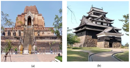
Figure 1. Original images: (a) Wat Chedi Luang, (b) Matsue Castle.

Peak signal-to-noise ratio (PSNR) [43] and signal-to-noise ratio (SNR) [44] were used as the metrics for evaluating the performance of each algorithm. The PSNR and SNR at $x_n$ are given by

$$\begin{array}{c}\hfill PSNR\left(x_n\right)=10{log}_{10}\left(\frac{MA{X}^2}{MSE}\right),\end{array}$$

(40)

$$\begin{array}{c}\hfill SNR\left(x_n\right)=10{log}_{10}\left(\frac{\parallel x-\overline{x}{\parallel }_2}{\parallel x_n-\overline{x}{\parallel }_2}\right),\end{array}$$

(41)

where $MAX$ is the maximum pixel value (usually 255 in 8-bit grayscale images) and $MSE=\frac{1}{{256}^2}{\parallel x_n-x\parallel }_2^2$ is the mean squared error between the original and the distorted image. Both and SNR are expressed in decibels (dB) as a logarithmic measure of the signal-to-noise or signal-to-error ratio.

In image restoration, both PSNR and SNR are commonly used as metrics to assess the performance of deblurring results. However, it is important to note that these metrics provide different types of information.

PSNR measures the quality of a deblurred image by comparing it to the original image and evaluating the amount of noise introduced during the restoration process. It calculates the ratio between the peak signal power (the maximum possible value for the pixel) and the mean squared error (MSE) between the original and deblurred images. Higher PSNR values indicate better restoration quality as they indicate a lower level of distortion or noise.

On the other hand, SNR measures the ratio between the signal power and the noise power in the deblurred image. It quantifies the preservation of the original signal after the restoration process. Higher SNR values indicate less noise in the deblurred image.

While both PSNR and SNR are useful metrics, they focus on different aspects of image restoration. PSNR primarily considers the visual quality and fidelity of the deblurred image compared to the original, while SNR focuses more on the amount of noise present in the deblurred image.

To comprehensively evaluate the performance of your deblurring algorithm, it is recommended to consider both PSNR and SNR. They provide complementary information about the restoration quality.

We now employ our proposed algorithm (TIFB-BiGM) in Theorem 2 to solve the convex bilevel optimization problems (38) and (39). In our experiments, the algorithm developed in this paper (TIFB-BiGM) as well as the others are discussed and applied to solve the convex bilevel optimization problems (38) and (39), where $\omega \left(x\right)=\frac{1}{2}{\parallel x\parallel }_2^2$, ${\psi }_1\left(x\right)={\parallel v-Ax\parallel }^2$, ${\psi }_2\left(x\right)=\zeta {\parallel Wx\parallel }_1$ and $\zeta =5\times {10}^{-5}$. The observed images are blurred images. We compute the Lipschitz constant $L_{{\psi }_1}$ by using the maximum eigenvalues of the matrix $A^{⊺}A$.

For the first experiment, the parameters of the TIFB-BiGM are chosen as follows: ${\beta }_n=\frac{0.99n}{n+1}$, ${\gamma }_n=\frac{1}{50n}$, $c_n=\frac{1}{L_{{\psi }_1}}$, ${\tau }_n=\frac{{10}^{14}}{n^2}$ and $s=0.01$. Now, the experiments for recovering the “Wat Chedi Luang” image with size of $256\times 256$ using TIFB-BiGM with different inertial parameters are shown in Table 1 and Table 2. We also observe from Table 1 and Table 2 that ${\mu }_n$ tends to 1 and ${\rho }_n$ tends to 0

$${\mu }_n=\frac{0.99n}{n+0.001}\mathrm{and}{\rho }_n=\frac{1}{n^2}$$

gives the highest values of PSNR and SNR for our method.

Table 1. PSNR values for restoration of “Wat Chedi Luang” image by TIFB-BiGM after 300 iterations for different choices of parameters ${\mu }_n$ and ${\rho }_n$.

${\mathit{\mu }}_{\mathit{n}}\to$	0.1	0.3	0.5	0.9	$\frac{0.99\mathit{n}}{\mathit{n}+0.001}$	1
${\mathit{\rho }}_{\mathit{n}}\downarrow$
0.1	22.9755	23.2143	23.5185	24.6769	25.3398	25.4489
0.3	22.7791	22.9764	23.2154	23.9454	24.2129	24.2479
0.5	22.6116	22.7799	22.9773	23.5215	23.6923	23.7133
0.9	22.3362	22.4662	22.6129	22.9789	23.0805	23.0924
$\frac{1}{n^2}$	23.0847	23.3513	23.7038	25.4271	26.2116	24.9267

Table 2. SNR values for restoration of “Wat Chedi Luang” image by TIFB-BiGM after 300 iterations for different choices of parameters ${\mu }_n$ and ${\rho }_n$.

${\mathit{\mu }}_{\mathit{n}}\to$	0.1	0.3	0.5	0.9	$\frac{0.99\mathit{n}}{\mathit{n}+0.001}$	1
${\mathit{\rho }}_{\mathit{n}}\downarrow$
0.1	18.9503	19.1890	19.4932	20.6516	21.3144	21.4236
0.3	18.7539	18.9510	19.1901	19.9200	20.1876	20.2225
0.5	18.5864	18.7545	18.9519	19.4961	19.6670	19.6879
0.9	18.3110	18.4408	18.5875	18.9536	19.0551	19.0670
$\frac{1}{n^2}$	19.0595	18.3260	19.6784	21.4018	22.1913	20.9014

The parameter values for each algorithm were chosen for optimum performance, based on the published literature. The value for ${\gamma }_n$ in Table 3 is the best choice for BiG-SAM considered in [13]. For iBiG-SAM, $\alpha =3$ is the best choice over other values considered in [17], and the same authors found, based on their numerical experiments, ${\mu }_n=\frac{n}{n+1}$ to be the best choice for FVFBA.

Table 3. Parameters selection of TIFB-BiGM, IVMSPA, FVFBA, BiG-SAM, and iBiG-SAM.

Methods	Setting
TIFB-BiGM	$s=0.01$, $c_n=\frac{1}{L_{{\psi }_1}}$, ${\beta }_n=\frac{0.99n}{n+1}$, ${\gamma }_n=\frac{1}{50n}$, ${\tau }_n=\frac{{10}^{18}}{n^2}$, ${\mu }_n=\frac{0.99n}{n+0.001}$, ${\rho }_n=\frac{1}{n^2}$
IVMSPA	$s=0.01$, $c_n=\frac{1}{L_f}$, ${\alpha }_n=\frac{1}{50n}$, ${\beta }_n={\gamma }_n=0.5$, ${\tau }_n=\frac{{10}^{20}}{n}$ $${\theta }_n=\left\{\begin{array}{cc}min\left\{\frac{p_n-1}{p_{n+1}},\frac{{\alpha }_n{\tau }_n}{∥x_n-x_{n-1}∥}\right\}\hfill & \hfill \mathrm{if}{x}_n\ne x_{n-1}\\ \frac{p_n-1}{p_{n+1}}\hfill & \hfill \mathrm{otherwise}\end{array}\right.$$ where $p_1=1$ and $p_{n+1}=\frac{1+\sqrt{1+4p_n^2}}{2}$
FVFBA	$c_n=\frac{n}{n+1}$, ${\beta }_n=\frac{0.99n}{n+1}$, ${\gamma }_n=\frac{1}{50n}$, ${\tau }_n=\frac{{10}^{15}}{n^2}$ $${\theta }_n=\left\{\begin{array}{cc}min\left\{\frac{n}{n+1},\frac{{\tau }_n}{∥x_n-x_{n-1}∥}\right\}\hfill & \mathrm{if}{x}_n\ne x_{n-1}\\ \frac{n}{n+1}\hfill & \mathrm{otherwise}\end{array}\right.$$
BiG-SAM	$\lambda =0.01$, $c=\frac{1}{L_{{\psi }_1}}$, ${\gamma }_n=\frac{2\left(0.1\right)}{1-n\frac{2+c{L}_{{\psi }_1}}{4}}$
iBiG-SAM	$\lambda =0.01$, $c=\frac{1}{L_{{\psi }_1}}$, ${\gamma }_n=\frac{2\left(0.1\right)}{1-\frac{2+c{L}_{{\psi }_1}}{4}}$, ${\beta }_n=\frac{{\gamma }_n}{n^{0.01}}$ $$\begin{array}{c}{\theta }_n=\left\{\begin{array}{cc}min\left\{\frac{n}{n+\alpha -1},\frac{{\beta }_n}{∥x_n-x_{n-1}∥}\right\}\hfill & \mathrm{if}{x}_n\ne x_{n-1},\hfill \\ \frac{n}{n+\alpha -1}\hfill & \mathrm{otherwise}\hfill \end{array}\right.\end{array}$$

The following experiments demonstrate Algorithm 2’s efficiency for image restoration in comparison to IVMSPA, FVFBA, BiG-SAM, and iBiG-SAM using PSNR and SNR as measurements.

The efficiency of restoring images using various algorithms under different iterations are illustrated in Figure 2, Figure 3, Figure 4, Figure 5, Figure 6 and Figure 7. The results indicate that TIFB-BiGM achieves higher PSNR and SNR values than IVMSPA, FVFBA, BiG-SAM, and iBiG-SAM. Therefore, our algorithm demonstrates superior convergence behavior compared to the aforementioned methods.

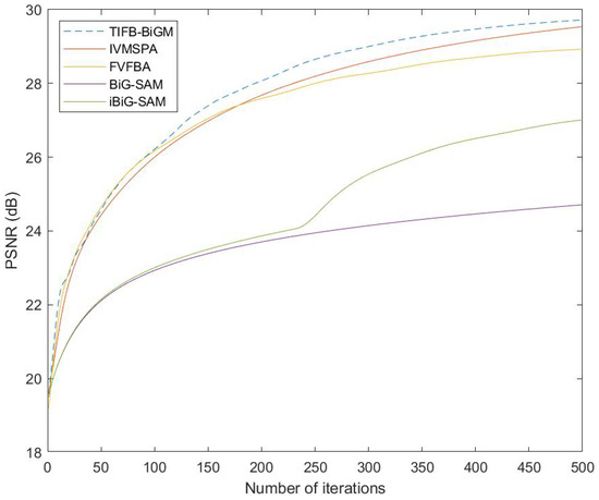
Figure 2. The graphs of PSNR of each algorithm for Wat Chedi Luang.

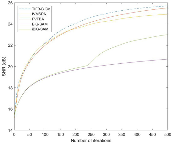
Figure 3. The graphs of SNR of each algorithm for Wat Chedi Luang.

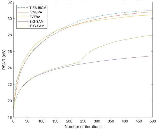
Figure 4. The graphs of PSNR of each algorithm for Matsue Castle.

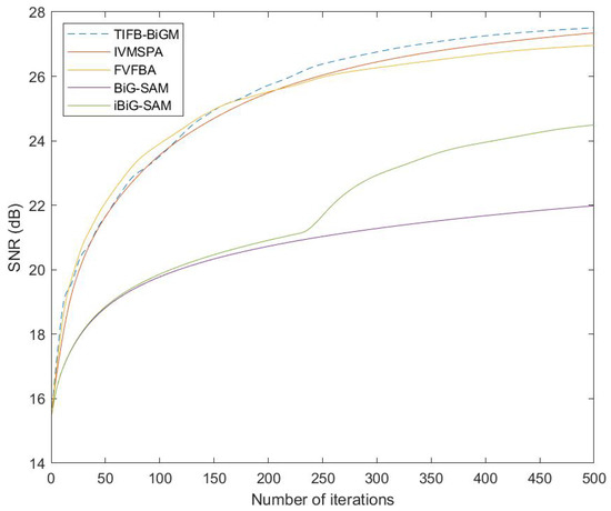
Figure 5. The graphs of SNR of each algorithm for Matsue Castle.

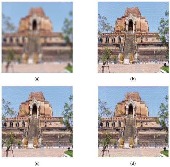
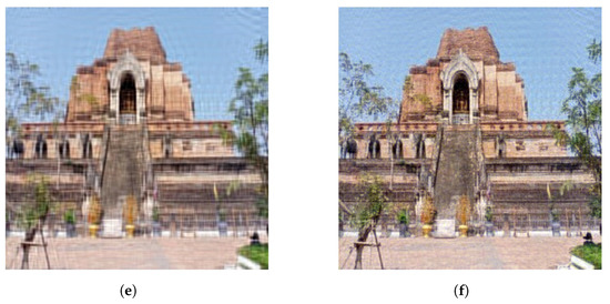
Figure 6. Results for deblurring “Wat Chedi Luang” image using various algorithms at the 500th iteration. (a) Gaussian blurred image, (b) TIFB-BiGM (PSNR = 29.7216, SNR = 25.6962), (c) IVMSPA (PSNR = 29.5375, SNR = 25.5121), (d) FVFBA (PSNR = 28.9243, SNR = 24.8989), (e) BiG-SAM (PSNR = 24.7118, SNR = 20.6864), and (f) iBiG-SAM (PSNR = 27.0172, SNR = 22.9918).

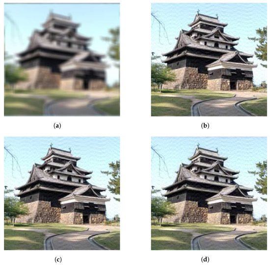
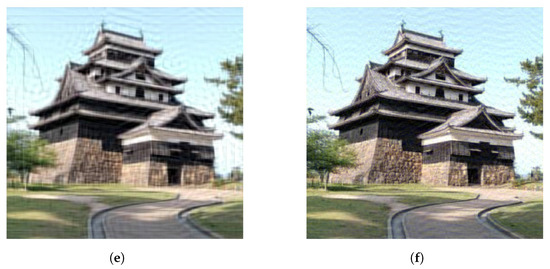
Figure 7. Results for deblurring “Matsue Castle” image using various algorithms at the 500th iteration. (a) Gaussian blurred image, (b) TIFB-BiGM (PSNR = 30.9830, SNR = 27.5075), (c) IVMSPA (PSNR = 30.8212, SNR = 27.3457), (d) FVFBA (PSNR = 30.43625, SNR = 26.9636), (e) BiG-SAM (PSNR = 25.4625, SNR = 21.9870), and (f) iBiG-SAM (PSNR = 27.9712, SNR = 24.4957).

5. Conclusions

In this paper, algorithmic solutions to a family of convex bilevel optimization problems are developed and applied to image processing. An interesting connection between minization problems and fixed-point methods is observed. We first present a modified two-step inertial viscosity algorithm (MTIVA) for finding a common fixed point of a family of nonexpansive operators in a Hilbert space and prove strong convergence under relatively mild conditions. This is the applied to the solution of a convex bilevel optimization problem by introducing a novel two-step inertial forward–backward bilevel gradient method (TIFB-BiGM). The main results are then employed in the solution of an image restoration problem. Through careful comparative analysis, we demonstrate that our algorithm outperforms several existing algorithms such as IVMSPA, FVFBA, BiG-SAM, and iBiG-SAM, in terms of image recovery efficiency, as verified through numerical experiments conducted under specific parameter settings.

There are several potential avenues for future research. Firstly, investigating the adaptability and performance of the proposed algorithm in different image processing tasks could provide valuable insights. Additionally, one might explore the algorithm’s scalability to large-scale image datasets or investigate the incorporation of parallel computing techniques that could enhance the algorithm’s computational efficiency. Moreover, conducting comparative studies with other state-of-the-art image restoration algorithms would provide a comprehensive evaluation of the algorithm’s strengths and limitations. Finally, exploring the applicability of the proposed algorithm to other domains beyond image processing, such as computer vision or signal processing, would broaden its potential impact.

References

- Franceschi, L.; Frasconi, P.; Salzo, S.; Grazzi, R.; Pontil, M. Bilevel programming for hyperparameter optimization and meta-learning. In Proceedings of the International Conference on Machine Learning (ICML), Stockholm, Sweden, 10–15 July 2018; pp. 1568–1577. [Google Scholar]
- Shaban, A.; Cheng, C.-A.; Hatch, N.; Boots, B. Truncated back-propagation for bilevel optimization. In Proceedings of the International Conference on Artificial Intelligence and Statistics (AISTATS), Okinawa, Japan, 16–18 April 2019; pp. 1723–1732. [Google Scholar]
- Kunapuli, G.; Bennett, K.P.; Hu, J.; Pang, J.-S. Classification model selection via bilevel programming. Optim. Methods Softw. 2008, 23, 475–489. [Google Scholar] [CrossRef]
- Flamary, R.; Rakotomamonjy, A.; Gasso, G. Learning constrained task similarities in graph regularized multitask learning. In Regularization, Optimization, Kernels, and Support Vector Machines; Chapman and Hall/CRC: Boca Raton, FL, USA, 2014; Volume 103, ISBN 978-0367658984. [Google Scholar]
- Konda, V.R.; Tsitsiklis, J.N. Actor-critic algorithms. In Proceedings of the Advances in Neural Information Processing Systems (NeurIPS), Denver, CO, USA, 30 November–2 December 1999; pp. 1008–1014. [Google Scholar]
- Bruck, R.E., Jr. On the weak convergence of an ergodic iteration for the solution of variational inequalities for monotone operators in Hilbert space. J. Math. Anal. Appl. 1977, 61, 159–164. [Google Scholar] [CrossRef]
- Lions, P.L.; Mercier, B. Splitting algorithms for the sum of two nonlinear operators. SIAM J. Numer. Anal. 1979, 16, 964–979. [Google Scholar] [CrossRef]
- Janngam, K.; Suantai, S. An inertial modified S-Algorithm for convex minimization problems with directed graphs and their applications in classification problems. Mathematics 2022, 10, 4442. [Google Scholar] [CrossRef]
- Cabot, A. Proximal point algorithm controlled by a slowly vanishing term: Applications to hierarchial minimization. SIAM J. Optim. 2005, 15, 555–572. [Google Scholar] [CrossRef]
- Xu, H.K. Averaged mappings and the gradient-projection algorithm. J. Optim. Theory Appl. 2011, 150, 360–378. [Google Scholar] [CrossRef]
- Passty, G.B. Ergodic convergence to a zero of the sum of monotone operators in Hilbert space. J. Math. Anal. Appl. 1979, 72, 383–390. [Google Scholar] [CrossRef]
- Beck, A.; Sabach, S. A first order method for finding minimal norm-like solutions of convex optimization problems. Math. Program. 2014, 147, 25–46. [Google Scholar] [CrossRef]
- Sabach, S.; Shtern, S. A first order method for solving convex bilevel optimization problems. SIAM J. Optim. 2017, 27, 640–660. [Google Scholar] [CrossRef]
- Nesterov, Y.E. A method for solving the convex programming problem with convergence rate O(1/k2). Sov. Math. Dokl. 1983, 27, 372–376. [Google Scholar]
- Polyak, B.T. Some methods of speeding up the convergence of iteration methods. USSR Comput. Math. Math. Phys. 1964, 4, 1–17. [Google Scholar] [CrossRef]
- Beck, A.; Teboulle, M. A fast iterative shrinkage-thresholding algorithm for linear inverse problems. SIAM J. Imaging Sci. 2009, 2, 183–202. [Google Scholar] [CrossRef]
- Shehu, Y.; Vuong, P.T.; Zemkoho, A. An inertial extrapolation method for convex simple bilevel optimization. Optim. Methods Softw. 2019, 36, 1–19. [Google Scholar] [CrossRef]
- Moudafi, A. Viscosity approximation method for fixed-points problems. J. Math. Anal. Appl. 2000, 241, 46–55. [Google Scholar] [CrossRef]
- Xu, H.K. Viscosity approximation methods for nonexpansive mappings. J. Math. Anal. Appl. 2004, 298, 279–291. [Google Scholar] [CrossRef]
- Takahashi, W. Viscosity approximation methods for countable families of nonexpansive mappings in Banach spaces. Nonlinear Anal. 2009, 70, 719–734. [Google Scholar] [CrossRef]
- Jailoka, P.; Suantai, S.; Hanjing, A. A fast viscosity forward–backward algorithm for convex minimization problems with an application in image recovery. Carpathian J. Math. 2021, 37, 449–461. [Google Scholar] [CrossRef]
- Janngam, K.; Suantai, S.; Cho, Y.J.; Kaewkhao, A.; Wattanataweekul, R. A Novel Inertial Viscosity Algorithm for Bilevel Optimization Problems Applied to Classification Problems. Mathematics 2023, 11, 3241. [Google Scholar] [CrossRef]
- Poon, C.; Liang, J. Geometry of First-order Methods and Adaptive Acceleration. arXiv 2020, arXiv:2003.03910. [Google Scholar]
- Liang, J. Convergence Rates of First-Order Operator Splitting Methods. Ph.D. Thesis, Normandie Universit’e, Normaundie, France, 2016. [Google Scholar]
- Poon, C.; Liang, J. Trajectory of Alternating Direction Method of Multiplier and Adaptive Acceleration. In Proceedings of the Advances in Neural Information Processing Systems, Vancouver, BC, Canada, 8–14 December 2019. [Google Scholar]
- Polyak, B.T. Introduction to Optimization; Optimization Software, Publication Division: New York, NY, USA, 1987. [Google Scholar]
- Combettes, P.L.; Glaudin, L. Quasi-Nonexpansive Iterations on the Affine Hull of Orbits: From Mann’s Mean Value Algorithm to Inertial Methods. SIAM J. Optim. 2017, 27, 2356–2380. [Google Scholar] [CrossRef]
- Nakajo, K.; Shimoji, K.; Takahashi, W. On strong convergence by the hybrid method for families of mappings in Hilbert spaces. Nonlinear Anal. 2009, 71, 112–119. [Google Scholar] [CrossRef]
- Aoyama, K.; Kimura, Y. Strong convergence theorems for strongly nonexpansive sequences. Appl. Math. Comput. 2011, 217, 7537–7545. [Google Scholar] [CrossRef]
- Aoyama, K.; Kohsaka, F.; Takahashi, W. Strong convergence theorems by shrinking and hybrid projection methods for relatively nonexpansive mappings in Banach spaces. Nonlinear Anal. Convex Anal. 2009, 10, 7–26. [Google Scholar]
- Moreau, J.J. Fonctions convexes duales et points proximaux dans un espace hilbertien. Comptes Rendus Acad. Sci. Paris Ser. A Math. 1962, 255, 2897–2899. [Google Scholar]
- Bauschke, H.H.; Combettes, P.L. Convex Analysis and Monotone Operator Theory in Hilbert Spaces; Springer: New York, NY, USA, 2011. [Google Scholar]
- Bussaban, L.; Suantai, S.; Kaewkhao, A. A parallel inertial S-iteration forward–backward algorithm for regression and classification problems. Carpathian J. Math. 2020, 36, 35–44. [Google Scholar] [CrossRef]
- Takahashi, W. Introduction to Nonlinear and Convex Analysis; Yokohama Publishers: Yokohama, Japan, 2009. [Google Scholar]
- Saejung, S.; Yotkaew, P. Approximation of zeros of inverse strongly monotone operators in Banach spaces. Nonlinear Anal. 2012, 75, 724–750. [Google Scholar] [CrossRef]
- Maurya, A.; Tiwari, R. A Novel Method of Image Restoration by using Different Types of Filtering Techniques. Int. J. Eng. Sci. Innov. Technol. 2014, 3, 124–129. [Google Scholar]
- Suseela, G.; Basha, S.A.; Babu, K.P. Image Restoration Using Lucy Richardson Algorithm For X-Ray Images. IJISET Int. J. Innov.Sci. Eng. Technol. 2016, 3, 280–285. [Google Scholar]
- Vogel, C.R. Computational Methods for Inverse Problems; SIAM: Philadelphia, PA, USA, 2002. [Google Scholar]
- Eldén, L. Algorithms for the Regularization of Ill-Conditioned Least Squares Problems. BIT Numer. Math. 1977, 17, 134–145. [Google Scholar] [CrossRef]
- Hansen, P.C.; Nagy, J.G.; O’Leary, D.P. Deblurring Images: Matrices, Spectra, and Filtering (Fundamentals of Algorithms 3) (Fundamentals of Algorithms); SIAM: Philadelphia, PA, USA, 2006. [Google Scholar]
- Tibshirani, R. Regression shrinkage and selection via the lasso. J. R. Stat. Soc. B Methodol. 1996, 58, 267–288. [Google Scholar] [CrossRef]
- Yatakoat, P.; Suantai, S.; Hanjing, A. On Some Accelerated Optimization Algorithms Based on Fixed Point and Linesearch Techniques for Convex Minimization Problems with Applications. Adv. Cont. Discr. Mod. 2022, 2022, 43:1–43:13. [Google Scholar] [CrossRef]
- Thung, K.; Raveendran, P. A survey of image quality measures. In Proceedings of the 2009 International Conference for Technical Postgraduates (TECHPOS), Kuala Lumpur, Malaysia, 14–15 December 2009; pp. 1–4. [Google Scholar]
- Chen, D.Q.; Zhang, H.; Cheng, L.Z. A fast fixed-point algorithmfixed-point algorithmfixed-point algorithmfixed-point algorithm for total variation deblurring and segmentation. J. Math. Imaging Vis. 2012, 43, 167–179. [Google Scholar] [CrossRef]
Disclaimer/Publisher’s Note: The statements, opinions and data contained in all publications are solely those of the individual author(s) and contributor(s) and not of MDPI and/or the editor(s). MDPI and/or the editor(s) disclaim responsibility for any injury to people or property resulting from any ideas, methods, instructions or products referred to in the content. |
© 2023 by the authors. Licensee MDPI, Basel, Switzerland. This article is an open access article distributed under the terms and conditions of the Creative Commons Attribution (CC BY) license (https://creativecommons.org/licenses/by/4.0/).