Abstract
The Redundancy Allocation Problem (RAP) is well-known in the field of reliability optimization. In this paper, RAP is investigated assuming that the distribution of the time to failure of the components has the form of an Erlang distribution with a time-dependent rate parameter and considering that the choice of redundancy for each subsystem can be none, active, standby or mixed. A genetic algorithm is used to solve the problem of optimal allocation. To analyze the effect of the time dependence, some numerical examples are worked out. Then, a case study of RAP from the literature is analyzed. The obtained results show that time dependence of the failure time distribution parameters can lead to significant differences in the optimal redundancy allocation.
Keywords:
reliability optimization; redundancy allocation problem; redundancy strategies; Erlang distribution; time-dependent failure rates; genetic algorithm MSC:
60E05; 90B25
1. Introduction
The reliability of a system can be improved at design by allocating redundant components to the subsystems. In a redundant system, when a working component fails, the failed component function is taken over by a redundant one which can provide the same function. The problem to do this optimally is called Redundancy Allocation Problem (RAP), which amounts to optimally selecting the redundant components to be allocated to the subsystems. The choice of the redundancy allocation strategy is driven by objectives, and/or subject to constraints, such as reliability, cost, volume and weight, depending on the system application. Then, RAP can be defined as the problem of selecting the number and type of the redundant components to allocate to the system, so to optimize a specific objective, such as system reliability, under given constraints, such as total system cost and weight.
The two redundancy strategies commonly considered in RAPs are “active” and “standby”, although one called “mixed” has been introduced relatively recently [1]. In the active redundancy strategy, all components start to work at time zero and a redundant component might be found already failed before it is called to operation. In the standby redundancy strategy, one component is active and the others (at least one component) are standby. The standby redundancy strategy comes in the three types: cold, warm and hot [2]. In cold-standby, redundant components do not fail before they are used. In warm-standby, redundant components are subject to failure even when they are dormant, but at a rate lower than that of the main component which is working. Finally, in hot-standby, redundant components are subject to failure even while dormant, at a rate equal to that of the main components. Without loss of generality of the analysis, among the standby strategies, the present paper considers the cold-standby redundancy strategy, only for simplicity of illustration. In the mixed redundancy strategy, more than one component can be active while some others (one or more) are standby. The mixed redundancy strategy tries to combine the advantages of both active and standby strategies. Indeed, it is a general form of the active and standby strategies. The mixed redundancy strategy can be used in most practical cases, but the active and standby redundancy strategies are also used in certain cases, due to their simple forms. In the standby and mixed redundancy strategies, a switching system has to be used to activate a standby redundant component.
Some researchers considered RAP with the same redundancy strategy for all subsystems in the system [3,4,5,6,7,8,9,10,11,12,13,14,15,16,17,18,19,20,21,22,23,24,25,26,27,28,29,30,31,32,33,34]. Following Coit [35], some researchers have turned to consider the redundancy strategy for each subsystem, either active or standby, as a decision variable that can be optimally determined by an optimization model [36,37,38,39,40,41,42,43]. The mixed redundancy strategy has also been considered as an alternative for the subsystems [44,45,46,47,48,49,50,51,52].
Other aspects come realistically into play in a RAP; these include the objective function, the states of the components and that of the entire system, the type of the components to be allocated to each subsystem, the reparability of the components, and so on. For example, RAPs may be considered with a single objective function, e.g., aiming to maximizing system reliability [1,3,4,5,6,7,8,9,10,11,27,28,30,31,35,36,37,39,40,41,44,46,47,48,53,54,55], minimizing total system cost [12,13,14,15] or maximizing/minimizing other parameters [16,29]. Alternatively, RAPs may consider multi-objective functions [18,19,20,21,22,23,24,25,32,34,38,42,45,50,56,57,58,59].
Regarding the components, they might be represented as binary or multi-state. In the binary state representation, the components can only be totally healthy or completely failed [1,3,4,5,6,7,8,9,10,11,12,13,17,18,19,20,21,22,23,25,26,27,28,29,30,31,32,33,34,35,40,41,43,44,45,46,47,48,53,55]; in the multi-state, the components might have other states, intermediate between these two [14,15,16,24,60,61,62,63,64,65]. The type of the components in the subsystems can be characterized from different viewpoints. For instance, allocation of either identical [1,3,4,5,6,7,12,18,19,20,35,36,40,45,46,53,54] or non-identical components to each subsystem might be allowed [8,9,10,11,13,14,15,16,17,21,22,25,27,28,33,37,41,44,48,49,62]. Moreover, the components characteristics, including their cost, weight and performance function, might be deterministic or uncertain functions [66]. From another aspect, the components can be repairable [14,15,20,24,26,30,56] or non-repairable [1,3,4,5,6,7,9,11,13,16,17,18,19,21,22,27,28,29,31,35,36,37,40,41,43,44,45,46,47,48,53,54,55]. In this regard, a comprehensive categorization of reliability optimization problems is provided in [67].
This paper considers the RAP for a system with identical binary components in each subsystem. The redundancy strategy for each subsystem is taken as the decision variable that can be active, standby or mixed, and the objective function requires system reliability to be maximized. Also, the distribution of the time to failure of the components is assumed to have the form of an Erlang distribution, whose rate parameter (λ(t)) is not constant in time. To the best of our knowledge, no RAP with these novel realistic properties has ever been investigated in the literature.
The failure of the components allocated to a system may be due to degradation or due to occurrence of some shocks. In the case where component failure is due to shock occurrence, the Erlang distribution can be considered suitable for modeling the stochastic time to failure of the components. If the distribution of the time to failure of a component is considered as an Erlang distribution with a shape parameter of k, it means that the failure of the component is due to the occurrence of some shocks, so that the component will fail as soon as the kth shock occurs. So, the problem is of practical interest, for example for electronic components which often fail due to some shocks. In the Erlang distribution, the rate parameter indicates the rate of occurrence of the shocks. The rate parameter is usually assumed to be constant, to describe the failure of components subject to shocks occurring at a constant rate. But the occurrence rate of the shocks may not be constant in time and, for this reason, in this paper the rate parameter is considered time-dependent, λ(t).
The main contribution of this paper is to propose a model in which the rate parameter of the time to failure distribution of the components is time-dependent and the redundancy allocation strategy for the subsystems can be mixed or other redundancy strategies.
The rest of the paper is structured as follows. In Section 2, the mathematical formulation of the RAP is described in detail. A solution method based on a genetic algorithm is proposed in Section 3. A numerical example is elaborated in Section 4 with and without time dependence, to demonstrate the effect of the time dependence of the rate parameter. Then, a case study taken from literature is considered. Finally, the conclusions and the suggestions for future work are given in Section 5.
2. Materials and Methods
2.1. Problem Formulation
A single-objective RAP is considered, in which the distribution of the time to failure of any component has the form of an Erlang distribution. The main specificities are the time-dependent parameter λ(t) in the time to failure distribution function and the redundancy strategy of any subsystem that can select among active, standby, mixed or no redundancy strategies. Figure 1 depicts the structure of a system composed of a series of five subsystems.
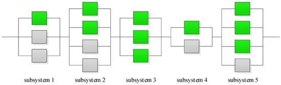
Figure 1.
Structure of a system of redundant subsystems.
A number of redundant components can be allocated to each subsystem, each of which may be active or standby. In Figure 1, the active components are shown in green and the standby ones are shown in grey. The purpose of allocating the redundant components is to increase the reliability of the subsystems and consequently to increase the reliability of the system. But, the existence of some physical and/or economical restrictions makes it impossible to allocate any desired number of components to the subsystems. Therefore, the goal is to determine the best choices including determining the type and number of active and standby components allocated to each subsystem so that the reliability of the system is maximized, under given constraints.
The number of active and standby components allocated to each subsystem determines the redundancy strategy. If no redundant component is allocated to a subsystem, the subsystem has no redundancy strategy. The redundancy strategy of a subsystem is active if all of the components allocated to the subsystem are active. If one of the components allocated to a subsystem is active and the rest are standby, the redundancy strategy is standby, and if more than one allocated component is active and one or more components are standby, the redundancy strategy is mixed. Since the number of active and standby components allocated to each subsystem is a decision variable, the redundancy strategy is also a decision variable that is determined during the optimization process.
In Figure 1, the redundancy strategy for each subsystem can be determined according to the number of active and standby components allocated to the subsystem. Accordingly, the redundancy strategy for subsystems 1 and 4 is standby, that for subsystems 2 and 5 is mixed, and the one for subsystem 3 is active. Before addressing the mathematical model, the assumptions considered and the notations used are presented below.
2.1.1. Notation
| ) | |
| number of subsystems | |
| number of active components allocated to subsystem i | |
| number of standby components allocated to subsystem i | |
| ) | |
| ) | |
| reliability at time t of the component (all identical) allocated to subsystem i | |
| shape parameter of the Erlang distribution for the component allocated to subsystem i | |
| rate parameter of the Erlang distribution for the component allocated to subsystem i | |
| cost and weight of the component allocated to subsystem i | |
| cost and weight of the switching system used in subsystem i (if present) | |
| maximum allowed amount for the system weight and cost | |
| switching system reliability at time t for subsystem i (if present) | |
| pdf of the jth failure time of standby components allocated to subsystem i at time t | |
| pdf of time to failure of the last active component allocated to subsystem i at time t | |
| pdf of the time to failure of the component allocated to subsystem i at time t | |
| cdf of the time to failure of the component allocated to subsystem i at time t | |
| average rate of occurrence of events between times a and b () | |
| number of events occurred until time t. |
2.1.2. Assumptions
As previously mentioned, the objective is to maximize the reliability of a system under a given number of constraints. The following assumptions are made:
- The components and the entire system are binary, i.e., they can be either totally healthy or completely failed.
- Components failures are independent events that individually cause no damage to the system.
- The redundancy strategy for each subsystem is a decision variable that can be selected to be active, standby, mixed or none.
- The distribution of the time to failure of the components has the form of an Erlang distribution with a time-dependent parameter λ(t).
- The components are non-repairable and there is no preventive maintenance.
- The components of each subsystem are identical, i.e., mixing of component types is not allowed.
2.1.3. Mathematical Model
The mathematical model for the considered problem can be formulated as follows:
Equation (1) expresses the objective of maximizing the system reliability by determining the type and the number of active and standby components allocated to each subsystem of the system. Constraints (2) and (3) express the maximum cost and weight for the entire system, respectively, whereas constraint set (4) considers the maximum number of components that can be allocated to each subsystem. The reliability of a system composed of a series of subsystems can be calculated as in Equation (5):
where NR represents subsystems with no redundancy strategy, whereas Active, Standby and Mixed represent those with active, standby and mixed redundancy strategies, respectively. As previously mentioned, the redundancy strategy for each subsystem is determined according to the number of active and standby components allocated. Therefore, the number of active and standby components allocated to each subsystem determines in which part of Equation (5) the reliability calculation of the subsystem should be placed. After determining the redundancy strategy for each subsystem, the reliability of the subsystems at time t is calculated with one of the following equations:
In these equations, ri(t) is the reliability of the components used in subsystem i at time t, ni is the number of components allocated to subsystem i, ρi(t) is the reliability of the switching system at time t, is the pdf of the time to failure of the jth component in subsystem i in standby and mixed redundancy strategies, whereas nA,i and nS,i represent the numbers of active and standby components assigned to subsystem i, respectively, in the case a mixed redundancy strategy is used (in this case nis = nA,i + nS,i), and is the pdf of the time to failure of the last active component in subsystem i in the mixed redundancy strategy.
In Equation (6), the reliability of subsystem i with no redundancy strategy is equal to the reliability of the only component allocated. In Equation (7), the reliability of subsystem i at time t with an active redundancy strategy is equal to the probability that at least one of the allocated components can remain healthy until time t. In Equation (8), the reliability of subsystem i at time t with standby redundancy strategy consists of two parts. The first part is the reliability of the active component allocated and the second one is equal to the sum of the probabilities that the jth standby component fails at time u (a time before t) and the next standby component is activated by the switching system at this time and can be healthy until time t. In Equation (9), the reliability of subsystem i at time t with a mixed redundancy strategy consist of three parts. The first part is equal to the probability that at least one of the active components remains healthy until time t. The second part is equal to the probability that the last active component fails at time u (a time before t) and the first standby component is activated by the switching system at this time and can remain healthy until time t. The third part is equal to the sum of the probabilities that the last active component fails at time v (a time before t) and, then, the standby components will be activated one by one after the failure of the previous one, until the jth standby component fails at time u (a time between v and t), and the next standby component is activated by the switching system at this time and can remain healthy until time t.
In Equation (9), can be calculated using Equation (10):
For example, if , can be calculated as in Equation (11):
If the time to failure of a component in subsystem i follows an Erlang distribution, then its reliability at time t is given by Equation (12):
When the time to failure of a generic component follows an Erlang distribution with shape parameter k, this component is, then, exposed to shocks that follow a Poisson distribution, and fails at the occurrence of the kth shock. The reliability of the component at time t is, therefore, the probability that less than k shocks occur until time t.
Considering that the times to failure of the components follow Erlang distribution, the reliability of subsystem i with no redundancy strategy and with an active redundancy strategy is obtained as Equations (13) and (14), respectively:
If the redundancy strategy of subsystem i is standby, considering that is a non-increasing function, we have:
The reliability formulation for a subsystem with a mixed redundancy strategy is slightly more complicated than the others. In Equation (9), we can rewrite ri(t) and Fi(t) as in Equation (12). Also, we know that for a component with Erlang time to failure distribution of shape parameter ki, fi(t)dt is the probability that ki − 1 shocks occur before time t and the kith shock occurs at time t. So, we can write fi(t)dt so as to explicitly represent that ki − 1 shocks occur before time t and one shock occurs between time t and t + dt:
For , the pdf of the time to failure of the jth component in subsystem i, we have:
This means that is the probability that j.ki − 1 shocks occur before time t and one shock occurs between time t and t + dt. So, if the redundancy strategy of subsystem i is mixed, the reliability of subsystem i, whose components times to failure follow an Erlang distribution, can be calculated as in Equation (18):
In this paper, it is assumed that the rate parameter is not constant, but a function of time, i.e., we have λ(t) instead of λ. So, the components will be exposed to shocks with a variable rate over time. For a nonhomogeneous Poisson process with rate λ(t), we have:
where
and N(t) is the number of events occurring prior to time t. Therefore, the reliability at time t for a component exposed to the shocks that follow a nonhomogeneous Poisson distribution, i.e., the probability that less than k shocks occur until time t, can be calculated as in Equation (21):
Now, if the rate parameter is time-dependent (λ(t)), by replacing by in Equations (13)–(15) and (18), the reliability of the subsystems with no redundancy strategy, and of those with active, standby and mixed redundancy strategies can be written as Equations (22)–(25), respectively:
2.2. RAP Solution Method
RAP is a problem of NP-hard class [68], and a meta-heuristic algorithm is here developed to search for the optimal solution. The genetic algorithm (GA) is a well-known meta-heuristic method for solving combinatorial optimization problems [69] and, indeed, it has been successfully employed for solving optimization problems in various fields [1,4,5,6,8,24,30,38,41,42,43,44,45,46,47,56]. In the following, the deployment of the algorithm for the solution of the proposed RAP is briefly described.
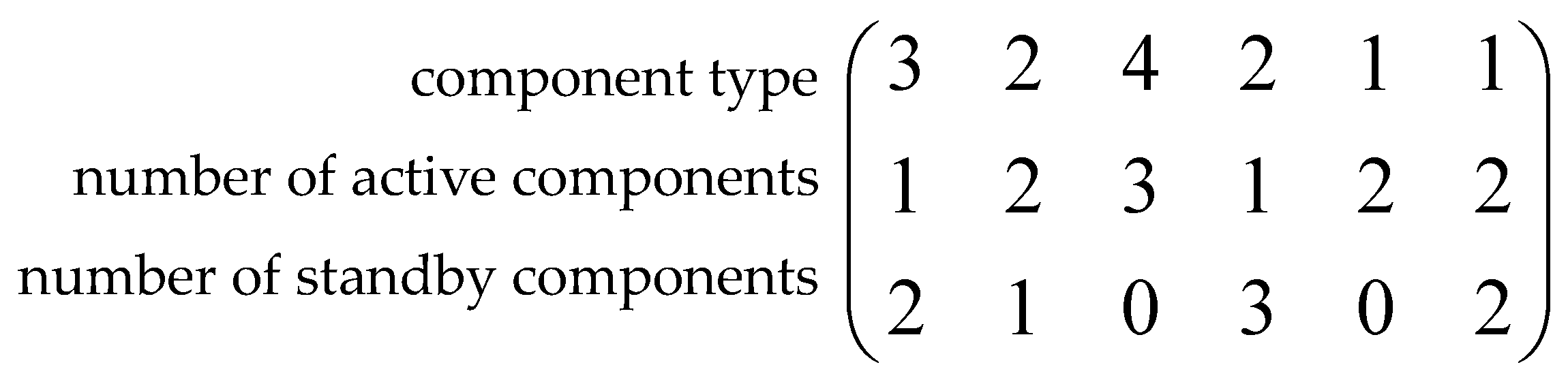
2.2.1. Solution Encoding (Chromosome)
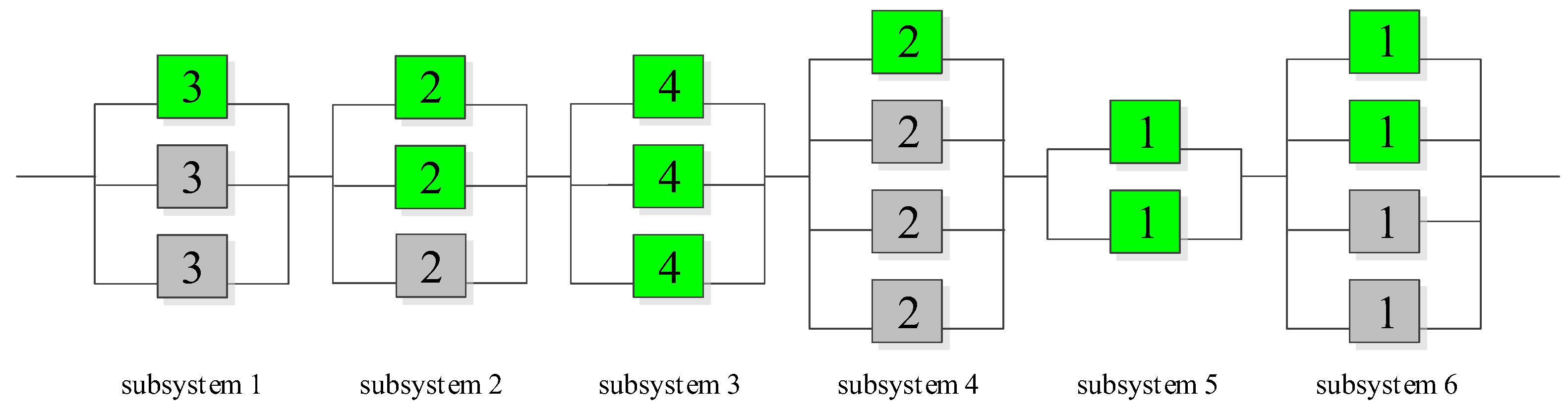
Solution encoding in the GA used is a 3 × s matrix, in which s represents the number of the subsystems in the system. For each subsystem, the first row is the type of selected component and the second and third rows give the numbers of allocated active and standby components, respectively. There is no need to add a row for the redundancy strategy, as it may be determined using the second and third rows: if the number of standby components is equal to zero, then the redundancy strategy is active (or no redundancy strategy, in case the number of active components is equal to one); if the number of active components is equal to one and there are some standby components, then the redundancy strategy is standby; finally, if the number of active components is larger than one and there are also some standby components, then the redundancy strategy is mixed. Figure 2 shows an example for the solution encoding with s = 6 subsystems. In the Figure, the active components are shown in green and the standby ones are shown in grey. As it can be seen in the Figure, the redundancy strategy for subsystems 1 and 4 is standby, that for subsystems 2 and 6 is mixed, and that for subsystems 3 and 5 is active. Figure 3 represents the structure of the system.

Figure 2.
Chromosome representation.
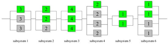
Figure 3.
Structure of the system corresponding to the solution in Figure 2.
2.2.2. Initial Population
The initial population is composed of the nPop solution matrix, whose entries are generated randomly. The solution matrices should be generated in such a way that in each column (subsystem), the first element is an integer number between 1 and the number of components types available for the subsystem, and the second and third elements are integer numbers so that their summation is less than or equal to the maximum number of components allowed for the subsystem.
2.2.3. Fitness Function
The fitness function is defined as the system reliability minus the penalty for constraints violation. Indeed, if a solution goes beyond the constraints, a large enough amount of penalty is deducted from the fitness function to guarantee that the final optimal solution is feasible. The amount of the penalty is equal to the product of the total amount of violations of the constraints and a fixed number. This penalty also allows the algorithm to search in the infeasible space for maintaining appropriate diversity in the search.
2.2.4. Selection
At each iteration, new offspring are generated by implementation of the crossover and mutation operators. The roulette wheel selection method is used to select the parents [8,40]. In the roulette wheel selection method, selection of the parents occurs based on their fitness function value: in other words, a solution is selected with probability proportional to its fitness function. After the selection process, the crossover and mutation operators are performed.
2.2.5. Crossover Operator
The crossover operator activates at a prespecified rate, rc. To explore a large variety of solutions, use has been made of different types of single-point, double-point, uniform and max–min crossover operators [1,4,44], each with a predetermined probability.
2.2.6. Mutation Operator
The mutation operator is implemented at a prespecified rate, rm. The main purpose of using this operator is to not get caught in the local optimal solutions. In this paper, use has been made of the random and max–min mutations [1,4,44], each with a predetermined probability.
To create the next generation, the offspring generated by implementation of the crossover and mutation operators are combined with the current population and the nPop best ones are selected. These best solutions, then, form the next-generation population.
2.2.7. Stopping Criteria
The GA is terminated after a prespecified number of iterations, MaxIt.
3. Results
As a numerical example, the new optimization model proposed in this paper is applied to three simple systems composed of series subsystems, for each of which some component choices are available for selection. The first system consists of 6 subsystems and the second one consists of 15 subsystems. The objective is to maximize system reliability at a mission time t = 100 (in arbitrary units). The third example is a case study introduced in [6]. The system is a pharmaceutical plant containing 10 series subsystems as follows:
| 1. Weighting machine, | 2. Sifter machine, | 3. Mass machine, |
| 4. Granulator, | 5. Fluid bed dryer, | 6. Octagonal blender, |
| 7. Rotary compression machine, | 8. Coating machine, | 9. Air compressor, |
| 10. Strip packing machine. |
In this work, we extend this case study so that the rate parameters for the time to failure of the components are time-dependent. The mission time is equal to t = 1000.
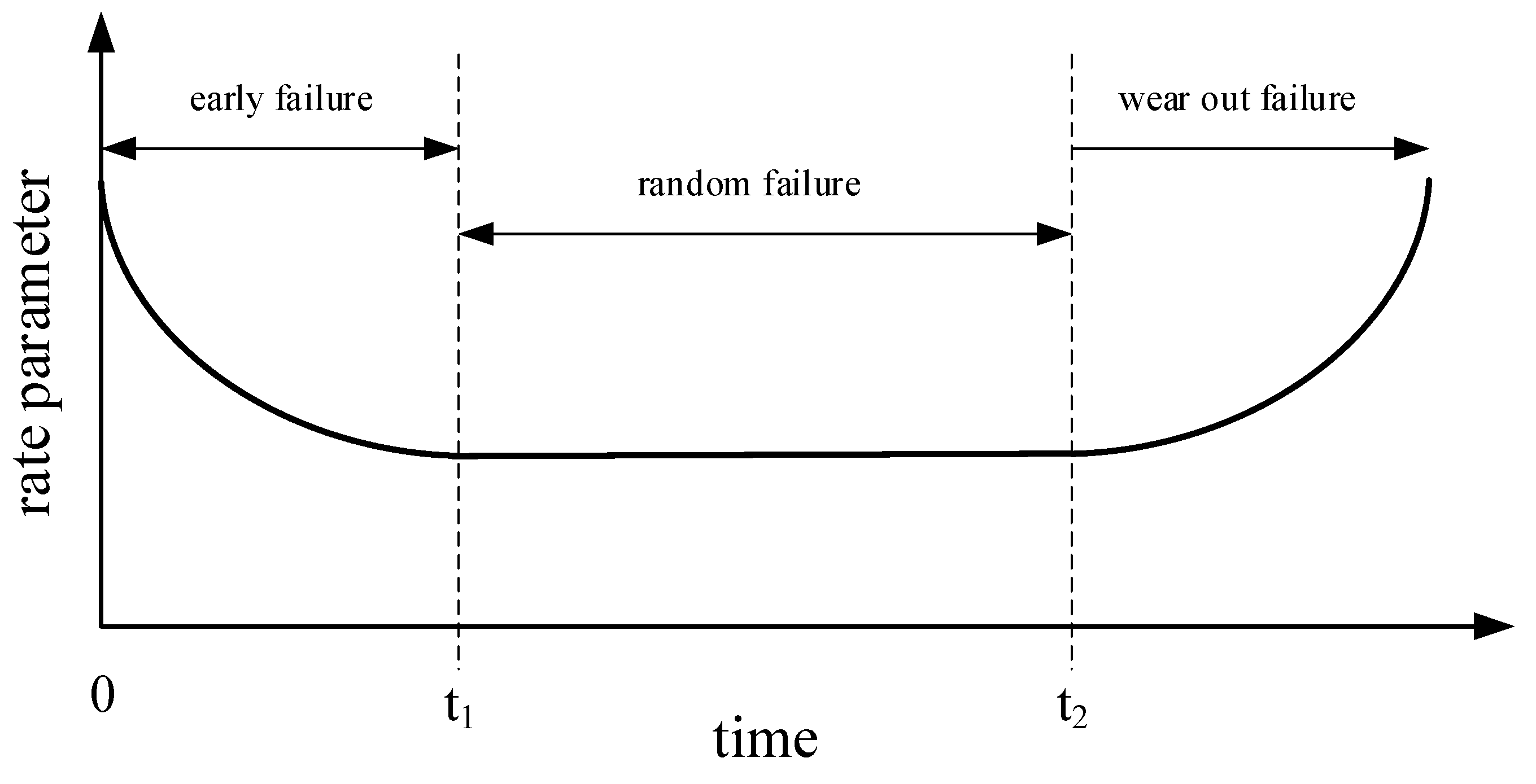
The rate parameter of the Erlang distribution is assumed to be in the form of a bathtub curve [70,71,72,73,74], as shown in Figure 4. As can be seen, the rate parameter first decreases over time, representing infant mortality, i.e., the process for which defective items fail early and the occurrence rate of the shocks decreases over time as the defective items are weeded out of the population. Then, the rate parameter remains constant for a period of time, as fully random shocks are the cause of failure, independent of time. Finally, the rate parameter increases, due to the aging process, for which the components are more likely to fail as time goes on.
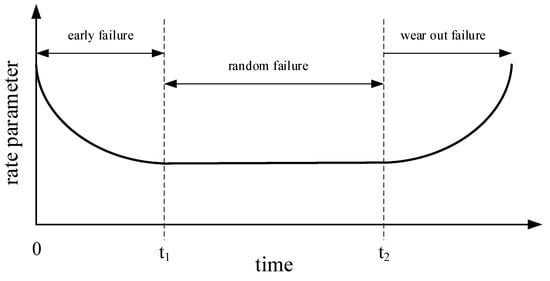
Figure 4.
Rate parameter (bathtub curve).
We consider the mathematical form of the rate parameter as in Equation (26) to describe all three parts, decreasing, constant and increasing:
In the above equation, c is a positive constant parameter. Different values of the parameter α allow representing the different parts of the rate parameter: a value of indicates a rate parameter decreasing over time; indicates a constant rate parameter over time; indicates a rate parameter increasing over time. Then, the rate parameter for the components in Figure 4 can be expressed by Equation (27), in which α1 is a value less than one and α2 is a value larger than one:
In this equation, the values of c1 and c2 should be determined so that the rate function is continuous at points t1 and t2. For this purpose, their values should be considered as given in Equation (28):
According to Equation (28), can be calculated as Equation (29) to be used in Equations (22)–(25).
The parameters α1, α2, t1 and t2 must be determined for each component type allocated in each subsystem. The components characteristics, including cost, weight and rate parameters, for the numerical examples are presented in Table A1, Table A2 and Table A3 in Appendix A. The values of C, W, reliability of the switching system at mission time and the maximum number of components that can be allocated to each subsystem are provided in Table A4 (in Appendix A) for the examples considered.
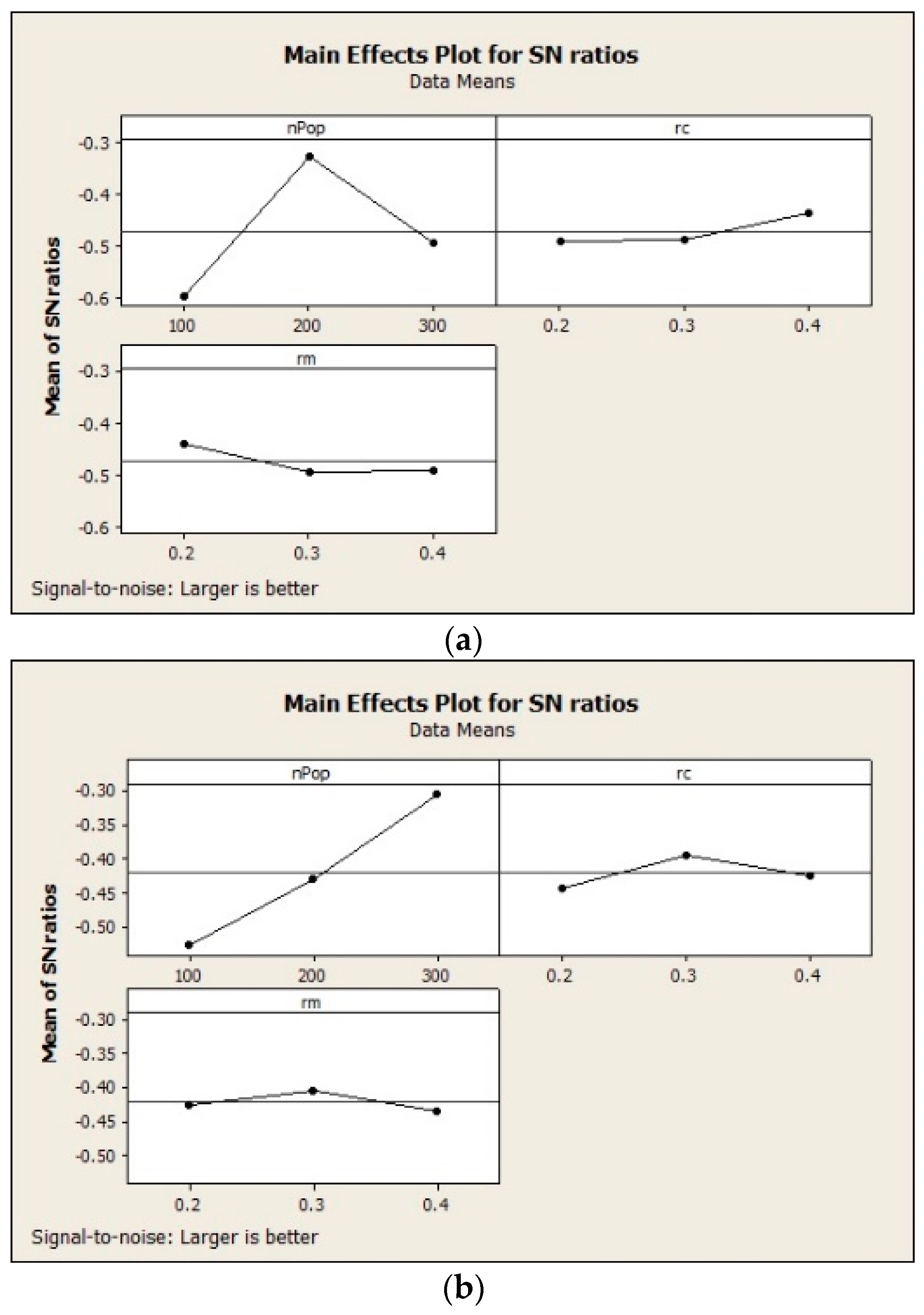
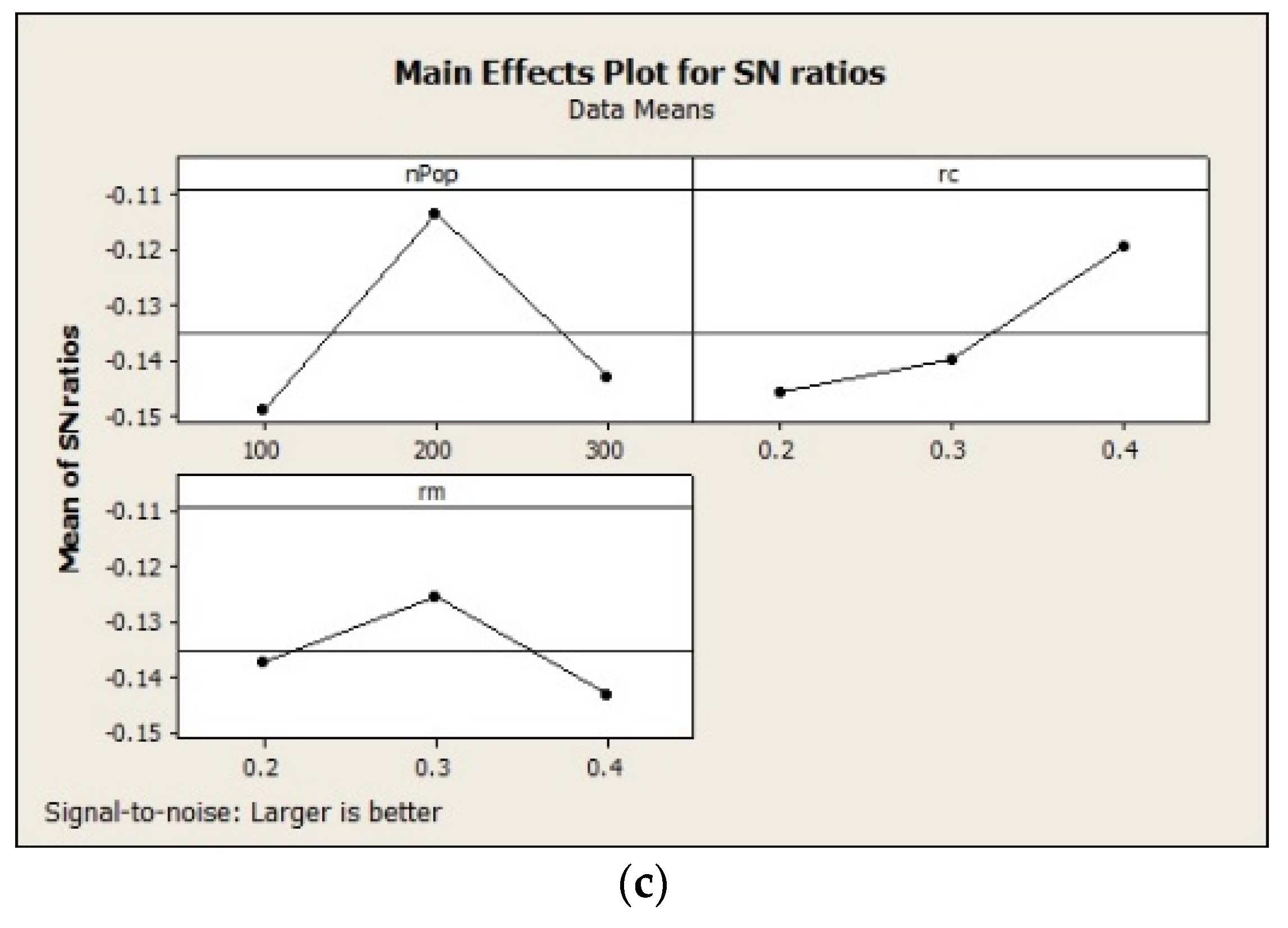
In order to tune the parameters of the GA, the Taguchi method has been used. For this purpose, three levels have been considered for population size, crossover rate and mutation rate.
The results obtained by the implementation of the Taguchi method are shown in Figure 5. The considered levels, as well as the best values obtained by this method for population size, crossover rate and mutation rate are shown in Table 1. The number of iterations is set to be MaxIt = 100 for all the examples.
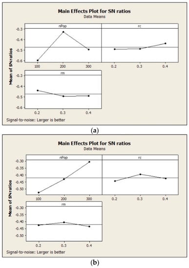
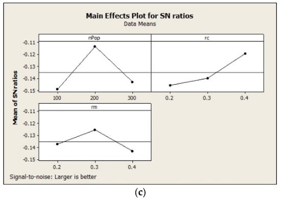
Figure 5.
The results obtained by the implementation of Taguchi method: (a) first example; (b) second example; (c) third example.

Table 1.
The results obtained by the implementation of Taguchi method.
As the GA is a stochastic algorithm, 20 trials of the algorithm are performed for each example and the best solution found amongst them is selected as the optimal solution. The trend of the algorithm towards the optimal solution in the 20 trials is shown in Figure A1, Figure A2 and Figure A3 in Appendix A. In order to show the robustness of the algorithm, the values of the minimum, maximum, average, standard deviation and coefficient of variation values of the reliability, weight and cost of the system in the optimal solutions obtained by different trials are reported in Table 2. The values of the reliability, weight and cost of the system in the optimal solutions obtained by different trials are reported in Table A5, Table A6 and Table A7 in Appendix A.
Table 2.
The results obtained by different trials.
To the best of our knowledge, there is no benchmark problem to compare with the RAP presented in this paper. So, to show the effect of time dependence of the rate parameter, the above-mentioned examples have also been considered with a constant rate parameter (i.e., useful lifetime), of the same value for all components. The best solutions obtained for the examples by considering a constant rate parameter (λ) and by considering a time-dependent rate parameter (λ(t)) (i.e., also initial early failure and final wear-out parts of the lifetime) are given in Table 3, Table 4 and Table 5.
Table 3.
Optimal solution with time dependence and without time dependence; first example.
Table 4.
Optimal solution with time dependence and without time dependence; second example.
Table 5.
Optimal solution with time dependence and without time dependence; third example.
4. Discussion
In this paper, a formulation for RAP is proposed in which the redundancy strategy for each subsystem is taken as the decision variable and the distribution of the time to failure of the components is assumed to have the form of an Erlang distribution, whose rate parameter (λ(t)) is not constant in time. Then, the genetic algorithm is proposed to search for the optimal solution.
As a numerical example, the proposed model was applied to three simple systems composed of series subsystems. As the GA is a stochastic algorithm, 20 trials of the algorithm were performed for each example. The trend of the algorithm towards the optimal solution was shown in Figure A1, Figure A2 and Figure A3. Due to the random nature of the GA, the trend of the algorithm towards the optimal solution varies in different trials. But, it can be seen that the differences are small, which shows the robustness of the algorithm in finding the optimal solution. It can also be seen that, in all three numerical examples, the different trials have converged to a similar solution, with only a slight difference, which shows the convergence of the algorithm to a same optimal solution.
Also, the results obtained by different trials including the values of the minimum, maximum, average, standard deviation and coefficient of variation of the reliability, the weight and cost of the system in the optimal solutions were reported in Table 2. As can be seen, the values of the coefficient of variation of the reliability, cost and weight of the system are small. This shows that the optimal solutions obtained by different trials are only slightly different from each other, which confirms the robustness of the algorithm in finding the optimal solution and its convergence to the optimal solution.
Since we did not find any benchmark problem to compare with the RAP presented in this paper, to show the effect of time dependence of the rate parameter, the examined examples have also been considered with a constant rate parameter, of the same value for all components. By comparing the best solution obtained for the problems with a constant rate parameter and with a time-dependent rate parameter (given in Table 3, Table 4 and Table 5), it can be seen that the structure of the obtained solutions, the type of components allocated to the subsystems and the redundancy strategy of the subsystems may be different.
For example, in the first numerical example, the type of the component allocated to the first subsystem is different in the cases of time-dependent rate parameter and constant rate parameter. In the case with time dependence, component type 3 is allocated to this subsystem, and in the case without time dependence, component type 2 is allocated to this subsystem. In this subsystem, the number of standby components is also different. In the case with time dependence, three standby components are allocated, and in the case without time dependence, one standby component is allocated to this subsystem. As another example, in the first numerical example, the redundancy strategy of the third subsystem is different in the two considered cases. In the case with time dependence, the redundancy strategy is active and, therefore, no switching system is required, but in the case without time dependence, the redundancy strategy is standby and, therefore, a switching system is required. These differences can also be seen in other cases.
In general, it can be seen that the structure of the optimal solution is different in the two cases. In other words, the optimal solution obtained in the case with time dependence is not optimal in the case without time dependence and vice versa. This issue is important in considering assumptions in designing a system. Because, if the rate parameter is variable over time, by considering it as constant, the real optimal solution cannot be found and, therefore, the system designed based on the considered assumptions is no longer optimal and its reliability in practice will be lower than what is theoretically expected. Therefore, to reach a real optimal solution, correct assumptions should be made.
In addition to the difference in the structure of the subsystems, there are also differences in the values of reliability, weight and cost in the obtained optimal solutions at the system level. For the cases studied, the obtained results show that, when the rate parameters are considered as time-dependent, the system reliability is lower. This is expected, because when the time-dependent rate parameters are considered for the components, the failure rates in the early and wear-out parts of the lifetime are higher than the failure rates in the useful part of the lifetime. Therefore, the probability of failure of the components is larger and, as a result, the reliability of the system is smaller than with constant failure rates. This decrease in reliability of the system in the case with time dependence is even accompanied by an increase in the cost of the system in some cases. For example, in the first numerical example, in the case with time dependence, the system reliability is 0.9702 and the system cost is 45, but in the case without time dependence, the system reliability is 0.9877 and the system cost is 37. This means that if the rate parameter is time-dependent, the system cost is higher than the case of a constant rate parameter but the system reliability is lower.
All of these confirm that it is important to consider the actual time-dependence of the rate parameter according to reality.
5. Conclusions
A redundancy allocation problem with multiple redundancy types has been investigated, in which the distribution of time to failure of the components has the form of an Erlang distribution with time-dependent parameter λ(t). The mathematical model has been formulated and a genetic algorithm has been developed to find the optimal solution.
To demonstrate the effect of time dependence of the time to failure distribution, numerical examples have been worked out with and without time dependence of the rate parameter. In the cases studied, it has been shown that taking the time dependence of the parameter λ(t) into account changes the reliability of the components and as a result, both the optimal redundancy structure of the subsystems of the system and the values of its reliability, cost and weight are different from those of the case with constant rate parameter.
In this paper, only identical components have been assumed to be allocated to each subsystem. However, mixing non-identical components might lead to improved system reliability; so, it is suggested that future studies examine the effect of mixing non-identical components. Another aspect to consider is the uncertainty in the characteristics and the time to failure distribution parameters of the components. Considering multi-state, repairable components, other pdfs for the times to failure of the components and/or preventive maintenance is another interesting area for future investigation.
Since the model presented in each research needs to be compared with the previous ones, it can be useful to define benchmark problems that can show the impact of the assumptions of each model well and be used in future research. Therefore, the definition of suitable benchmark problems to be used in the research in this field can also be a suggestion for future research.
Author Contributions
Conceptualization, E.Z. and H.G.; Investigation, E.Z. and H.G.; Methodology, H.G.; Software, H.G.; Supervision, E.Z.; Validation, E.Z. and H.G.; Writing—original draft, H.G.; Writing—review and editing, E.Z. All authors have read and agreed to the published version of the manuscript.
Funding
This research received no external funding.
Institutional Review Board Statement
Not applicable.
Informed Consent Statement
Not applicable.
Data Availability Statement
In this of article, no new data were created.
Conflicts of Interest
The authors declare no conflict of interest.
Appendix A
Table A1.
Component data for the first numerical example.
Table A1.
Component data for the first numerical example.
| Component Type 1 (j = 1) | Component Type 2 (j = 2) | Component Type 3 (j = 3) | Component Type 4 (j = 4) | |||||||||||||||||||||||||||||
|---|---|---|---|---|---|---|---|---|---|---|---|---|---|---|---|---|---|---|---|---|---|---|---|---|---|---|---|---|---|---|---|---|
| i | λ0ij | α1ij | α2ij | t1ij | t2ij | kij | cij | wij | λ0ij | α1ij | α2ij | t1ij | t2ij | kij | cij | wij | λ0ij | α1ij | α2ij | t1ij | t2ij | kij | cij | wij | λ0ij | α1ij | α2ij | t1ij | t2ij | kij | cij | wij |
| 1 | 0.052 | 0.3 | 3 | 10 | 90 | 6 | 2 | 4 | 0.007 | 0.1 | 2 | 12 | 90 | 2 | 2 | 4 | 0.049 | 0.4 | 2 | 10 | 100 | 4 | 3 | 2 | 0.081 | 0.3 | 3 | 10 | 80 | 4 | 3 | 4 |
| 2 | 0.017 | 0.5 | 2 | 15 | 120 | 4 | 2 | 5 | 0.110 | 0.4 | 4 | 18 | 100 | 4 | 3 | 5 | 0.124 | 0.3 | 3 | 5 | 75 | 6 | 2 | 6 | 0.046 | 0.1 | 5 | 5 | 75 | 4 | 4 | 3 |
| 3 | 0.043 | 0.4 | 4 | 8 | 110 | 5 | 3 | 4 | 0.056 | 0.6 | 3 | 20 | 110 | 6 | 4 | 5 | 0.028 | 0.7 | 4 | 10 | 95 | 3 | 3 | 5 | 0.004 | 0.5 | 4 | 15 | 100 | 2 | 2 | 4 |
| 4 | 0.026 | 0.4 | 3 | 12 | 80 | 4 | 4 | 6 | 0.001 | 0.3 | 5 | 8 | 80 | 1 | 3 | 8 | 0.004 | 0.6 | 3 | 12 | 85 | 1 | 3 | 4 | 0.009 | 0.4 | 2 | 20 | 120 | 2 | 3 | 6 |
| 5 | 0.023 | 0.6 | 5 | 6 | 70 | 3 | 2 | 4 | 0.077 | 0.8 | 2 | 15 | 85 | 4 | 2 | 6 | 0.133 | 0.3 | 3 | 7 | 90 | 5 | 2 | 5 | 0.122 | 0.7 | 3 | 17 | 85 | 7 | 4 | 5 |
| 6 | 0.011 | 0.7 | 7 | 9 | 95 | 3 | 4 | 5 | 0.083 | 0.2 | 3 | 14 | 95 | 5 | 5 | 4 | 0.035 | 0.2 | 2 | 15 | 110 | 3 | 2 | 6 | 0.043 | 0.3 | 3 | 14 | 90 | 4 | 5 | 8 |
Table A2.
Component data for the second numerical example.
Table A2.
Component data for the second numerical example.
| Subsystem | Component Type | λ0ij | α1ij | α2ij | t1ij | t2ij | kij | cij | wij |
|---|---|---|---|---|---|---|---|---|---|
| i = 1 | 1 | 0.014 | 0.5 | 5 | 20 | 70 | 3 | 4 | 2 |
| 2 | 0.034 | 0.4 | 6 | 7 | 80 | 5 | 4 | 3 | |
| 3 | 0.014 | 0.2 | 4 | 10 | 110 | 2 | 3 | 6 | |
| 4 | 0.052 | 0.2 | 2 | 7 | 85 | 7 | 5 | 4 | |
| 5 | 0.048 | 0.3 | 3 | 16 | 85 | 8 | 2 | 6 | |
| 6 | 0.013 | 0.4 | 3 | 6 | 75 | 2 | 3 | 4 | |
| 7 | 0.021 | 0.1 | 4 | 5 | 100 | 3 | 4 | 2 | |
| 8 | 0.045 | 0.3 | 3 | 19 | 80 | 7 | 5 | 5 | |
| 9 | 0.023 | 0.3 | 5 | 18 | 80 | 4 | 5 | 8 | |
| 10 | 0.071 | 0.7 | 5 | 5 | 90 | 7 | 2 | 4 | |
| i = 2 | 1 | 0.027 | 0.5 | 3 | 8 | 100 | 3 | 5 | 3 |
| 2 | 0.017 | 0.4 | 4 | 16 | 105 | 2 | 3 | 3 | |
| 3 | 0.105 | 0.2 | 6 | 11 | 80 | 8 | 2 | 4 | |
| 4 | 0.019 | 0.8 | 3 | 19 | 80 | 3 | 2 | 6 | |
| 5 | 0.029 | 0.7 | 3 | 10 | 80 | 3 | 3 | 4 | |
| 6 | 0.049 | 0.5 | 4 | 19 | 80 | 6 | 4 | 5 | |
| 7 | 0.053 | 0.8 | 3 | 11 | 105 | 5 | 2 | 6 | |
| 8 | 0.046 | 0.1 | 5 | 14 | 90 | 7 | 5 | 8 | |
| 9 | 0.017 | 0.8 | 3 | 6 | 80 | 2 | 5 | 5 | |
| 10 | 0.023 | 0.7 | 6 | 10 | 80 | 3 | 4 | 3 | |
| i = 3 | 1 | 0.071 | 0.6 | 5 | 10 | 85 | 8 | 2 | 8 |
| 2 | 0.018 | 0.3 | 3 | 7 | 95 | 2 | 2 | 8 | |
| 3 | 0.022 | 0.6 | 3 | 15 | 85 | 2 | 5 | 2 | |
| 4 | 0.034 | 0.6 | 2 | 18 | 85 | 4 | 2 | 4 | |
| 5 | 0.021 | 0.5 | 2 | 12 | 70 | 2 | 5 | 8 | |
| 6 | 0.019 | 0.2 | 6 | 16 | 70 | 4 | 5 | 4 | |
| 7 | 0.071 | 0.6 | 4 | 15 | 95 | 8 | 3 | 7 | |
| 8 | 0.051 | 0.8 | 5 | 20 | 85 | 6 | 4 | 2 | |
| 9 | 0.063 | 0.6 | 5 | 11 | 105 | 7 | 5 | 6 | |
| 10 | 0.018 | 0.4 | 2 | 10 | 70 | 2 | 4 | 2 | |
| i = 4 | 1 | 0.021 | 0.8 | 6 | 6 | 105 | 2 | 2 | 7 |
| 2 | 0.014 | 0.1 | 4 | 14 | 90 | 3 | 3 | 6 | |
| 3 | 0.025 | 0.1 | 2 | 13 | 95 | 5 | 2 | 3 | |
| 4 | 0.032 | 0.2 | 4 | 20 | 105 | 5 | 2 | 5 | |
| 5 | 0.047 | 0.3 | 3 | 11 | 75 | 4 | 3 | 2 | |
| 6 | 0.017 | 0.1 | 4 | 10 | 80 | 3 | 2 | 7 | |
| 7 | 0.049 | 0.1 | 4 | 5 | 75 | 4 | 5 | 6 | |
| 8 | 0.051 | 0.3 | 5 | 17 | 85 | 8 | 3 | 8 | |
| 9 | 0.021 | 0.7 | 6 | 20 | 75 | 3 | 2 | 7 | |
| 10 | 0.043 | 0.2 | 5 | 20 | 95 | 7 | 4 | 6 | |
| i = 5 | 1 | 0.073 | 0.5 | 3 | 10 | 85 | 8 | 5 | 3 |
| 2 | 0.048 | 0.5 | 5 | 10 | 85 | 6 | 3 | 2 | |
| 3 | 0.022 | 0.2 | 4 | 6 | 105 | 3 | 2 | 3 | |
| 4 | 0.055 | 0.8 | 3 | 11 | 85 | 6 | 3 | 8 | |
| 5 | 0.054 | 0.2 | 6 | 11 | 95 | 8 | 5 | 7 | |
| 6 | 0.017 | 0.3 | 3 | 10 | 100 | 2 | 2 | 8 | |
| 7 | 0.032 | 0.6 | 5 | 6 | 95 | 4 | 3 | 2 | |
| 8 | 0.063 | 0.3 | 6 | 12 | 90 | 9 | 4 | 4 | |
| 9 | 0.051 | 0.7 | 6 | 10 | 90 | 6 | 4 | 8 | |
| 10 | 0.073 | 0.5 | 4 | 7 | 105 | 9 | 2 | 2 | |
| i = 6 | 1 | 0.016 | 0.8 | 2 | 19 | 95 | 2 | 2 | 6 |
| 2 | 0.027 | 0.1 | 3 | 9 | 90 | 5 | 3 | 8 | |
| 3 | 0.012 | 0.2 | 5 | 20 | 90 | 2 | 2 | 3 | |
| 4 | 0.009 | 0.2 | 6 | 8 | 70 | 2 | 4 | 7 | |
| 5 | 0.051 | 0.7 | 5 | 20 | 70 | 7 | 5 | 7 | |
| 6 | 0.029 | 0.5 | 4 | 19 | 110 | 4 | 4 | 3 | |
| 7 | 0.027 | 0.8 | 4 | 8 | 105 | 3 | 3 | 7 | |
| 8 | 0.017 | 0.6 | 4 | 15 | 75 | 2 | 4 | 7 | |
| 9 | 0.021 | 0.7 | 4 | 15 | 85 | 2 | 3 | 4 | |
| 10 | 0.031 | 0.1 | 6 | 5 | 85 | 4 | 3 | 5 | |
| i = 7 | 1 | 0.032 | 0.5 | 6 | 9 | 70 | 6 | 4 | 7 |
| 2 | 0.022 | 0.2 | 2 | 9 | 100 | 3 | 3 | 6 | |
| 3 | 0.053 | 0.4 | 6 | 13 | 90 | 7 | 4 | 5 | |
| 4 | 0.017 | 0.7 | 2 | 14 | 95 | 2 | 5 | 5 | |
| 5 | 0.029 | 0.3 | 6 | 13 | 105 | 4 | 3 | 3 | |
| 6 | 0.034 | 0.1 | 4 | 13 | 90 | 7 | 4 | 8 | |
| 7 | 0.037 | 0.6 | 4 | 16 | 70 | 5 | 4 | 6 | |
| 8 | 0.051 | 0.3 | 6 | 20 | 75 | 8 | 3 | 8 | |
| 9 | 0.024 | 0.7 | 4 | 16 | 95 | 2 | 2 | 4 | |
| 10 | 0.015 | 0.4 | 2 | 20 | 90 | 2 | 3 | 5 | |
| i = 8 | 1 | 0.018 | 0.4 | 5 | 10 | 85 | 2 | 3 | 3 |
| 2 | 0.023 | 0.7 | 4 | 20 | 75 | 3 | 3 | 6 | |
| 3 | 0.012 | 0.2 | 7 | 8 | 110 | 2 | 2 | 4 | |
| 4 | 0.024 | 0.2 | 4 | 20 | 80 | 5 | 3 | 2 | |
| 5 | 0.02 | 0.2 | 4 | 11 | 90 | 3 | 5 | 3 | |
| 6 | 0.058 | 0.6 | 6 | 19 | 95 | 7 | 2 | 5 | |
| 7 | 0.061 | 0.6 | 4 | 6 | 70 | 8 | 2 | 4 | |
| 8 | 0.024 | 0.3 | 4 | 20 | 85 | 3 | 2 | 6 | |
| 9 | 0.068 | 0.7 | 3 | 12 | 105 | 7 | 3 | 2 | |
| 10 | 0.073 | 0.5 | 5 | 14 | 105 | 8 | 2 | 7 | |
| i = 9 | 1 | 0.049 | 0.7 | 2 | 8 | 85 | 5 | 5 | 7 |
| 2 | 0.068 | 0.6 | 6 | 11 | 85 | 8 | 2 | 7 | |
| 3 | 0.024 | 0.6 | 6 | 15 | 70 | 4 | 3 | 5 | |
| 4 | 0.019 | 0.2 | 3 | 10 | 90 | 2 | 3 | 7 | |
| 5 | 0.024 | 0.7 | 6 | 10 | 80 | 3 | 5 | 5 | |
| 6 | 0.049 | 0.7 | 3 | 13 | 75 | 6 | 3 | 5 | |
| 7 | 0.035 | 0.2 | 3 | 20 | 110 | 6 | 5 | 5 | |
| 8 | 0.025 | 0.8 | 3 | 7 | 80 | 3 | 3 | 6 | |
| 9 | 0.049 | 0.8 | 4 | 5 | 75 | 6 | 2 | 8 | |
| 10 | 0.039 | 0.2 | 2 | 14 | 90 | 5 | 4 | 5 | |
| i = 10 | 1 | 0.028 | 0.1 | 5 | 20 | 90 | 7 | 4 | 2 |
| 2 | 0.048 | 0.4 | 2 | 5 | 90 | 5 | 4 | 2 | |
| 3 | 0.019 | 0.2 | 2 | 20 | 105 | 3 | 3 | 4 | |
| 4 | 0.015 | 0.2 | 4 | 12 | 70 | 2 | 3 | 4 | |
| 5 | 0.018 | 0.3 | 4 | 6 | 85 | 2 | 5 | 5 | |
| 6 | 0.019 | 0.8 | 6 | 14 | 95 | 2 | 2 | 3 | |
| 7 | 0.058 | 0.3 | 6 | 15 | 80 | 8 | 3 | 8 | |
| 8 | 0.016 | 0.1 | 4 | 6 | 110 | 2 | 4 | 4 | |
| 9 | 0.051 | 0.5 | 6 | 11 | 70 | 9 | 2 | 6 | |
| 10 | 0.065 | 0.3 | 5 | 10 | 100 | 8 | 2 | 3 | |
| i = 11 | 1 | 0.033 | 0.6 | 5 | 14 | 80 | 4 | 3 | 3 |
| 2 | 0.027 | 0.3 | 2 | 5 | 85 | 3 | 3 | 7 | |
| 3 | 0.035 | 0.4 | 4 | 15 | 90 | 5 | 2 | 8 | |
| 4 | 0.009 | 0.1 | 2 | 10 | 110 | 2 | 5 | 8 | |
| 5 | 0.038 | 0.2 | 6 | 17 | 85 | 6 | 2 | 3 | |
| 6 | 0.035 | 0.3 | 3 | 20 | 110 | 5 | 3 | 3 | |
| 7 | 0.029 | 0.1 | 6 | 11 | 75 | 6 | 2 | 3 | |
| 8 | 0.022 | 0.6 | 3 | 10 | 70 | 3 | 2 | 3 | |
| 9 | 0.058 | 0.6 | 4 | 18 | 90 | 7 | 2 | 8 | |
| 10 | 0.062 | 0.2 | 3 | 11 | 90 | 8 | 2 | 2 | |
| i = 12 | 1 | 0.022 | 0.6 | 4 | 14 | 105 | 2 | 5 | 6 |
| 2 | 0.041 | 0.2 | 5 | 18 | 85 | 7 | 2 | 6 | |
| 3 | 0.037 | 0.5 | 6 | 6 | 95 | 4 | 3 | 4 | |
| 4 | 0.023 | 0.5 | 6 | 6 | 105 | 2 | 3 | 4 | |
| 5 | 0.032 | 0.6 | 6 | 18 | 90 | 4 | 2 | 4 | |
| 6 | 0.059 | 0.7 | 3 | 6 | 80 | 7 | 5 | 3 | |
| 7 | 0.038 | 0.3 | 3 | 20 | 80 | 6 | 5 | 4 | |
| 8 | 0.054 | 0.4 | 4 | 20 | 90 | 8 | 2 | 7 | |
| 9 | 0.057 | 0.7 | 4 | 5 | 100 | 5 | 2 | 3 | |
| 10 | 0.015 | 0.5 | 2 | 8 | 85 | 2 | 3 | 8 | |
| i = 13 | 1 | 0.047 | 0.8 | 3 | 11 | 95 | 5 | 2 | 7 |
| 2 | 0.019 | 0.5 | 3 | 12 | 75 | 2 | 5 | 5 | |
| 3 | 0.053 | 0.3 | 3 | 10 | 80 | 7 | 4 | 8 | |
| 4 | 0.039 | 0.6 | 2 | 11 | 70 | 4 | 5 | 3 | |
| 5 | 0.019 | 0.8 | 5 | 17 | 85 | 2 | 3 | 2 | |
| 6 | 0.048 | 0.4 | 2 | 11 | 90 | 6 | 2 | 6 | |
| 7 | 0.023 | 0.1 | 3 | 7 | 90 | 3 | 4 | 8 | |
| 8 | 0.034 | 0.1 | 4 | 6 | 80 | 5 | 3 | 7 | |
| 9 | 0.072 | 0.3 | 3 | 11 | 85 | 9 | 2 | 8 | |
| 10 | 0.051 | 0.8 | 2 | 20 | 85 | 5 | 4 | 3 | |
| i = 14 | 1 | 0.019 | 0.5 | 3 | 16 | 75 | 2 | 5 | 5 |
| 2 | 0.038 | 0.6 | 2 | 7 | 85 | 4 | 5 | 7 | |
| 3 | 0.045 | 0.3 | 5 | 19 | 85 | 7 | 5 | 6 | |
| 4 | 0.033 | 0.2 | 6 | 9 | 95 | 4 | 2 | 7 | |
| 5 | 0.045 | 0.4 | 3 | 12 | 105 | 6 | 4 | 2 | |
| 6 | 0.024 | 0.2 | 3 | 9 | 80 | 3 | 4 | 5 | |
| 7 | 0.023 | 0.8 | 3 | 8 | 110 | 3 | 2 | 4 | |
| 8 | 0.048 | 0.3 | 3 | 14 | 90 | 7 | 3 | 3 | |
| 9 | 0.024 | 0.8 | 3 | 14 | 85 | 3 | 5 | 8 | |
| 10 | 0.041 | 0.2 | 2 | 6 | 70 | 6 | 4 | 7 | |
| i = 15 | 1 | 0.021 | 0.8 | 4 | 14 | 75 | 2 | 4 | 2 |
| 2 | 0.041 | 0.4 | 7 | 11 | 90 | 5 | 5 | 3 | |
| 3 | 0.043 | 0.5 | 3 | 6 | 70 | 5 | 4 | 8 | |
| 4 | 0.025 | 0.6 | 4 | 16 | 110 | 3 | 3 | 3 | |
| 5 | 0.012 | 0.2 | 2 | 18 | 95 | 2 | 5 | 6 | |
| 6 | 0.039 | 0.8 | 4 | 7 | 75 | 4 | 5 | 4 | |
| 7 | 0.047 | 0.3 | 5 | 9 | 90 | 5 | 2 | 6 | |
| 8 | 0.013 | 0.2 | 6 | 14 | 95 | 2 | 2 | 6 | |
| 9 | 0.015 | 0.6 | 4 | 18 | 90 | 2 | 4 | 4 | |
| 10 | 0.044 | 0.2 | 6 | 16 | 75 | 8 | 2 | 3 |
Table A3.
Component data for the third example (pharmaceutical plant).
Table A3.
Component data for the third example (pharmaceutical plant).
| Component Type 1 | Component Type 2 | Component Type 3 | Component Type 4 | |||||||||||||||||||||||||||||
|---|---|---|---|---|---|---|---|---|---|---|---|---|---|---|---|---|---|---|---|---|---|---|---|---|---|---|---|---|---|---|---|---|
| i | λ0ij × 105 | α1ij | α2ij | t1ij | t2ij | kij | cij | wij | λ0ij × 105 | α1ij | α2ij | t1ij | t2ij | kij | cij | wij | λ0ij × 105 | α1ij | α2ij | t1ij | t2ij | kij | cij | wij | λ0ij × 105 | α1ij | α2ij | t1ij | t2ij | kij | cij | wij |
| 1 | 128 | 0.5 | 5 | 200 | 880 | 3 | 16 | 26 | 176 | 0.8 | 2 | 50 | 840 | 3 | 20 | 19 | 276 | 0.6 | 3 | 140 | 860 | 5 | 18 | 17 | 607 | 0.9 | 4 | 190 | 1060 | 8 | 21 | 24 |
| 2 | 195 | 0.7 | 6 | 120 | 790 | 4 | 14 | 20 | 78 | 0.3 | 4 | 90 | 870 | 2 | 21 | 23 | 92 | 0.7 | 2 | 100 | 1000 | 2 | 13 | 26 | 430 | 0.1 | 4 | 80 | 1010 | 9 | 19 | 18 |
| 3 | 419 | 0.6 | 3 | 220 | 1050 | 7 | 20 | 24 | 473 | 0.8 | 5 | 150 | 1090 | 7 | 15 | 17 | 368 | 0.2 | 6 | 80 | 720 | 8 | 16 | 26 | 455 | 0.8 | 2 | 240 | 1010 | 7 | 17 | 27 |
| 4 | 480 | 0.5 | 4 | 90 | 850 | 7 | 19 | 22 | 388 | 0.7 | 6 | 120 | 990 | 6 | 17 | 24 | 394 | 0.9 | 7 | 80 | 750 | 8 | 20 | 17 | 159 | 0.1 | 8 | 90 | 780 | 5 | 19 | 21 |
| 5 | 495 | 0.7 | 6 | 80 | 820 | 8 | 14 | 19 | 173 | 0.5 | 7 | 70 | 990 | 3 | 18 | 22 | 97 | 0.5 | 7 | 150 | 900 | 2 | 19 | 19 | 88 | 0.9 | 5 | 190 | 840 | 2 | 18 | 24 |
| 6 | 101 | 0.2 | 6 | 150 | 850 | 3 | 15 | 23 | 106 | 0.1 | 2 | 210 | 940 | 4 | 13 | 26 | 194 | 0.2 | 4 | 70 | 980 | 4 | 20 | 19 | 68 | 0.2 | 6 | 210 | 930 | 2 | 14 | 22 |
| 7 | 68 | 0.3 | 7 | 180 | 830 | 2 | 14 | 26 | 245 | 0.5 | 7 | 160 | 800 | 5 | 15 | 18 | 241 | 0.2 | 8 | 240 | 760 | 8 | 21 | 23 | 455 | 0.9 | 3 | 100 | 820 | 7 | 14 | 22 |
| 8 | 194 | 0.2 | 4 | 220 | 1070 | 5 | 18 | 23 | 189 | 0.2 | 5 | 220 | 920 | 5 | 14 | 26 | 205 | 0.3 | 4 | 70 | 870 | 4 | 16 | 20 | 190 | 0.3 | 4 | 90 | 1100 | 4 | 20 | 25 |
| 9 | 265 | 0.8 | 6 | 50 | 780 | 5 | 21 | 27 | 415 | 0.8 | 5 | 240 | 830 | 7 | 15 | 19 | 293 | 0.7 | 3 | 210 | 1000 | 5 | 16 | 26 | 429 | 0.3 | 5 | 250 | 820 | 9 | 20 | 18 |
| 10 | 99 | 0.1 | 2 | 170 | 1050 | 4 | 14 | 18 | 597 | 0.6 | 4 | 90 | 840 | 9 | 15 | 25 | 213 | 0.7 | 6 | 150 | 910 | 4 | 21 | 23 | 452 | 0.2 | 4 | 120 | 990 | 8 | 18 | 25 |
Table A4.
Values of C, W, nmax,i and ρi(t) for the examples.
Table A4.
Values of C, W, nmax,i and ρi(t) for the examples.
| C | W | nmax,i | ρi (t) | |
|---|---|---|---|---|
| First example | 50 | 70 | 6 | 0.99 |
| Second example | 310 | 400 | 6 | 0.99 |
| Third example | 480 | 519 | 6 | 0.99 |
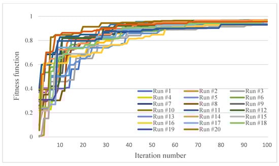
Figure A1.
Trend of GA towards the optimal solution in 20 different trials; first example.
Figure A1.
Trend of GA towards the optimal solution in 20 different trials; first example.


Figure A2.
Trend of GA towards the optimal solution in 20 different trials; second example.
Figure A2.
Trend of GA towards the optimal solution in 20 different trials; second example.
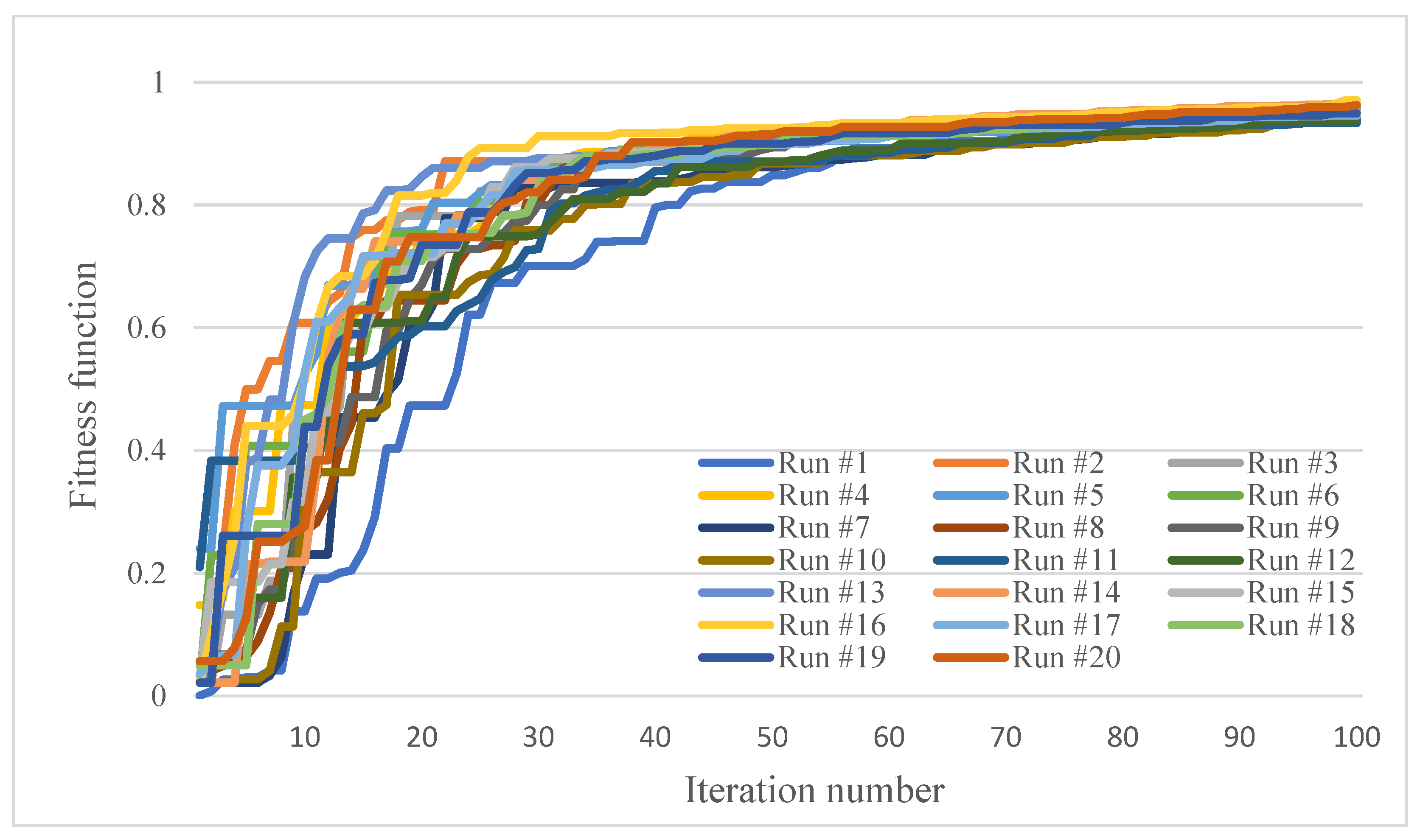

Figure A3.
Trend of GA towards the optimal solution in 20 different trials; third example.
Figure A3.
Trend of GA towards the optimal solution in 20 different trials; third example.
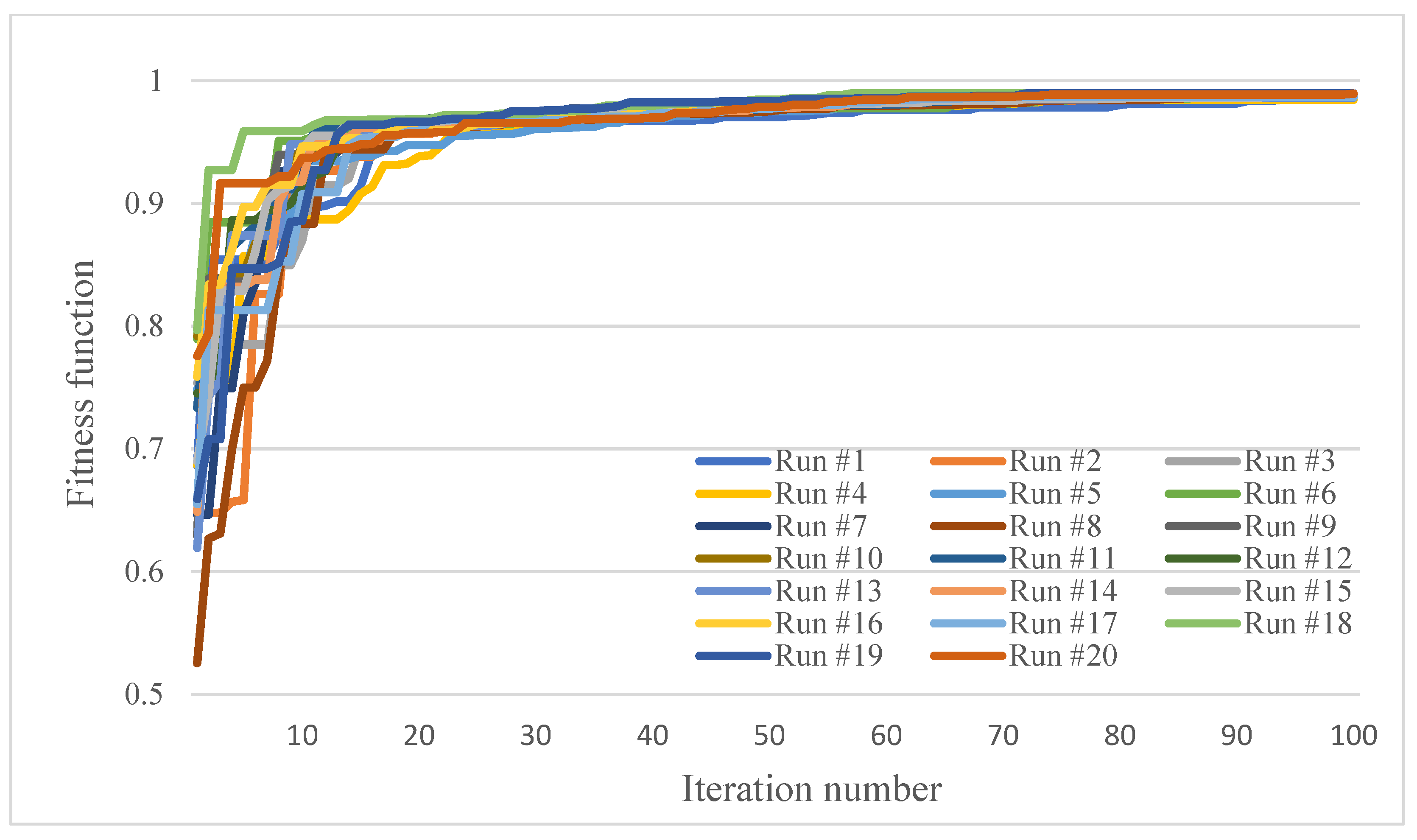
Table A5.
Details of the optimal solutions obtained by different trials; first example.
Table A5.
Details of the optimal solutions obtained by different trials; first example.
| System Characteristics | |||
|---|---|---|---|
| Iteration Number | Reliability | Cost | Weight |
| 1 | 0.9612 | 45 | 68 |
| 2 | 0.9541 | 37 | 70 |
| 3 | 0.9284 | 45 | 70 |
| 4 | 0.9578 | 39 | 68 |
| 5 | 0.9692 | 48 | 69 |
| 6 | 0.9702 | 45 | 70 |
| 7 | 0.9619 | 49 | 66 |
| 8 | 0.9662 | 46 | 68 |
| 9 | 0.9695 | 45 | 70 |
| 10 | 0.9652 | 50 | 70 |
| 11 | 0.9673 | 49 | 68 |
| 12 | 0.9669 | 49 | 68 |
| 13 | 0.9376 | 39 | 68 |
| 14 | 0.9689 | 48 | 69 |
| 15 | 0.934 | 47 | 66 |
| 16 | 0.9624 | 38 | 68 |
| 17 | 0.9549 | 47 | 65 |
| 18 | 0.9577 | 45 | 70 |
| 19 | 0.9315 | 46 | 69 |
| 20 | 0.9562 | 46 | 68 |
Table A6.
Details of the optimal solutions obtained by different trials; second example.
Table A6.
Details of the optimal solutions obtained by different trials; second example.
| System Characteristics | |||
|---|---|---|---|
| Iteration Number | Reliability | Cost | Weight |
| 1 | 0.9626 | 200 | 265 |
| 2 | 0.9506 | 306 | 367 |
| 3 | 0.9614 | 259 | 302 |
| 4 | 0.9557 | 251 | 380 |
| 5 | 0.9425 | 259 | 352 |
| 6 | 0.9584 | 250 | 337 |
| 7 | 0.9397 | 271 | 372 |
| 8 | 0.9574 | 303 | 319 |
| 9 | 0.9584 | 249 | 339 |
| 10 | 0.9351 | 242 | 325 |
| 11 | 0.9337 | 235 | 311 |
| 12 | 0.9384 | 237 | 298 |
| 13 | 0.9565 | 219 | 393 |
| 14 | 0.9643 | 248 | 333 |
| 15 | 0.9488 | 236 | 285 |
| 16 | 0.9707 | 272 | 282 |
| 17 | 0.946 | 240 | 323 |
| 18 | 0.9524 | 277 | 384 |
| 19 | 0.9493 | 302 | 384 |
| 20 | 0.9628 | 260 | 343 |
Table A7.
Details of the optimal solutions obtained by different trials; third example.
Table A7.
Details of the optimal solutions obtained by different trials; third example.
| System Characteristics | |||
|---|---|---|---|
| Iteration Number | Reliability | Cost | Weight |
| 1 | 0.9866 | 458 | 519 |
| 2 | 0.9865 | 448 | 518 |
| 3 | 0.9881 | 466 | 517 |
| 4 | 0.9846 | 478 | 518 |
| 5 | 0.9896 | 454 | 514 |
| 6 | 0.9894 | 453 | 516 |
| 7 | 0.9889 | 469 | 513 |
| 8 | 0.9881 | 469 | 519 |
| 9 | 0.9886 | 464 | 509 |
| 10 | 0.9894 | 453 | 516 |
| 11 | 0.9889 | 469 | 513 |
| 12 | 0.9869 | 471 | 512 |
| 13 | 0.9864 | 429 | 518 |
| 14 | 0.9896 | 454 | 514 |
| 15 | 0.9868 | 451 | 519 |
| 16 | 0.9891 | 468 | 510 |
| 17 | 0.9869 | 424 | 509 |
| 18 | 0.9896 | 467 | 517 |
| 19 | 0.9896 | 461 | 519 |
| 20 | 0.9894 | 453 | 516 |
References
- Ardakan, M.A.; Hamadani, A.Z. Reliability optimization of series–parallel systems with mixed redundancy strategy in subsystems. Reliab. Eng. Syst. Saf. 2014, 130, 132–139. [Google Scholar] [CrossRef]
- Ebeling, C.E. An Introduction to Reliability and Maintainability Engineering; Tata McGraw-Hill Education: New York, NY, USA, 2004. [Google Scholar]
- Hsieh, T.J. Hierarchical redundancy allocation for multi-level reliability systems employing a bacterial-inspired evolutionary algorithm. Inf. Sci. 2014, 288, 174–193. [Google Scholar] [CrossRef]
- Abouei Ardakan, M.; Mirzaei, Z.; Zeinal Hamadani, A.; Elsayed, E.A. Reliability Optimization by Considering Time-Dependent Reliability for Components. Qual. Reliab. Eng. Int. 2017, 33, 1641–1654. [Google Scholar] [CrossRef]
- Gupta, R.K.; Bhunia, A.K.; Roy, D. A GA based penalty function technique for solving constrained redundancy allocation problem of series system with interval valued reliability of components. J. Comput. Appl. Math. 2009, 232, 275–284. [Google Scholar] [CrossRef]
- Mellal, M.A.; Zio, E. System reliability-redundancy allocation by evolutionary computation. In Proceedings of the 2017 2nd International Conference on System Reliability and Safety (ICSRS) 2017, Milan, Italy, 20–22 December 2017; pp. 15–19. [Google Scholar]
- Coit, D.W. Cold-standby redundancy optimization for nonrepairable systems. Iie Trans. 2001, 33, 471–478. [Google Scholar] [CrossRef]
- Zhao, J.; Zeng, S.; Guo, J.; Yang, C. Redundancy allocation with non-identical component and uncertainty. In Proceedings of the 2015 Annual Reliability and Maintainability Symposium (RAMS) 2015, Palm Harbor, FL, USA, 26–29 January 2015; pp. 1–6. [Google Scholar]
- Liang, Y.C.; Smith, A.E. An ant colony optimization algorithm for the redundancy allocation problem (RAP). IEEE Trans. Reliab. 2004, 53, 417–423. [Google Scholar] [CrossRef]
- Onishi, J.; Kimura, S.; James, R.J.; Nakagawa, Y. Solving the redundancy allocation problem with a mix of components using the improved surrogate constraint method. IEEE Trans. Reliab. 2007, 56, 94–101. [Google Scholar] [CrossRef]
- Caserta, M.; Voß, S. An exact algorithm for the reliability redundancy allocation problem. Eur. J. Oper. Res. 2015, 244, 110–116. [Google Scholar] [CrossRef]
- Ramirez-Marquez, J.E.; Coit, D.W. A heuristic for solving the redundancy allocation problem for multi-state series-parallel systems. Reliab. Eng. Syst. Saf. 2004, 83, 341–349. [Google Scholar] [CrossRef]
- Sharma, V.K.; Agarwal, M.; Sen, K. Reliability evaluation and optimal design in heterogeneous multi-state series-parallel systems. Inf. Sci. 2011, 181, 362–378. [Google Scholar] [CrossRef]
- Lai, C.M.; Yeh, W.C. Two-stage simplified swarm optimization for the redundancy allocation problem in a multi-state bridge system. Reliab. Eng. Syst. Saf. 2016, 156, 148–158. [Google Scholar] [CrossRef]
- Li, Y.; Zio, E. A quantum-inspired evolutionary approach for non-homogeneous redundancy allocation in series-parallel multi-state systems. In Proceedings of the 2014 10th International Conference on Reliability, Maintainability and Safety (ICRMS) 2014, Guangzhou, China, 6–8 August 2014; pp. 526–532. [Google Scholar]
- Wang, Y.; Li, L. A PSO algorithm for constrained redundancy allocation in multi-state systems with bridge topology. Comput. Ind. Eng. 2014, 68, 13–22. [Google Scholar] [CrossRef]
- Hsieh, T.J.; Yeh, W.C. Penalty guided bees search for redundancy allocation problems with a mix of components in series–parallel systems. Comput. Oper. Res. 2012, 39, 2688–2704. [Google Scholar] [CrossRef]
- Garg, H.; Rani, M.; Sharma, S.P.; Vishwakarma, Y. Bi-objective optimization of the reliability-redundancy allocation problem for series-parallel system. J. Manuf. Syst. 2014, 33, 335–347. [Google Scholar] [CrossRef]
- Zhang, E.; Chen, Q. Multi-objective reliability redundancy allocation in an interval environment using particle swarm optimization. Reliab. Eng. Syst. Saf. 2016, 145, 83–92. [Google Scholar] [CrossRef]
- Guo, J.; Wang, Z.; Zheng, M.; Wang, Y. Uncertain multiobjective redundancy allocation problem of repairable systems based on artificial bee colony algorithm. Chin. J. Aeronaut. 2014, 27, 1477–1487. [Google Scholar] [CrossRef]
- Kulturel-Konak, S.; Coit, D.W. Determination of Pruned Pareto sets for the multi-objective system redundancy allocation problem. In Proceedings of the 2007 IEEE Symposium on Computational Intelligence in Multi-Criteria Decision-Making 2007, Honolulu, HI, USA, 1–5 April 2007; pp. 390–394. [Google Scholar]
- Mariano, C.H.; Kuri-Morales, A.F. Complex componential approach for redundancy allocation problem solved by simulation-optimization framework. J. Intell. Manuf. 2014, 25, 661–680. [Google Scholar] [CrossRef]
- Cao, D.; Murat, A.; Chinnam, R.B. Efficient exact optimization of multi-objective redundancy allocation problems in series-parallel systems. Reliab. Eng. Syst. Saf. 2013, 111, 154–163. [Google Scholar] [CrossRef]
- Sun, M.X.; Li, Y.F.; Zio, E. On the optimal redundancy allocation for multi-state series–parallel systems under epistemic uncertainty. Reliab. Eng. Syst. Saf. 2019, 192, 106019. [Google Scholar] [CrossRef]
- Valaei, M.R.; Behnamian, J. Allocation and sequencing in 1-out-of-N heterogeneous cold-standby systems: Multi-objective harmony search with dynamic parameters tuning. Reliab. Eng. Syst. Saf. 2017, 157, 78–86. [Google Scholar] [CrossRef]
- Bei, X.; Chatwattanasiri, N.; Coit, D.W.; Zhu, X. Combined redundancy allocation and maintenance planning using a two-stage stochastic programming model for multiple component systems. IEEE Trans. Reliab. 2017, 66, 950–962. [Google Scholar] [CrossRef]
- Dobani, E.R.; Ardakan, M.A.; Davari-Ardakani, H.; Juybari, M.N. RRAP-CM: A new reliability-redundancy allocation problem with heterogeneous components. Reliab. Eng. Syst. Saf. 2019, 191, 106563. [Google Scholar] [CrossRef]
- Hsieh, T.J. Component mixing with a cold standby strategy for the redundancy allocation problem. Reliab. Eng. Syst. Saf. 2021, 206, 107290. [Google Scholar] [CrossRef]
- Bhattacharyee, N.; Kumar, N.; Mahato, S.K.; Bhunia, A.K. Development of a blended particle swarm optimization to optimize mission design life of a series–parallel reliable system with time dependent component reliabilities in imprecise environments. Soft Comput. 2021, 25, 11745–11761. [Google Scholar] [CrossRef]
- Wang, W.; Wu, Z.; Xiong, J.; Xu, Y. Redundancy optimization of cold-standby systems under periodic inspection and maintenance. Reliab. Eng. Syst. Saf. 2018, 180, 394–402. [Google Scholar] [CrossRef]
- Mellal, M.A.; Zio, E. System reliability-redundancy optimization with cold-standby strategy by an enhanced nest cuckoo optimization algorithm. Reliab. Eng. Syst. Saf. 2020, 201, 106973. [Google Scholar] [CrossRef]
- Yeh, W.C.; Su, Y.Z.; Gao, X.Z.; Hu, C.F.; Wang, J.; Huang, C.L. Simplified swarm optimization for bi-objection active reliability redundancy allocation problems. Appl. Soft Comput. 2021, 106, 107321. [Google Scholar] [CrossRef]
- Yeh, W.C. BAT-based algorithm for finding all Pareto solutions of the series-parallel redundancy allocation problem with mixed components. Reliab. Eng. Syst. Saf. 2022, 228, 108795. [Google Scholar] [CrossRef]
- Kundu, P. A multi-objective reliability-redundancy allocation problem with active redundancy and interval type-2 fuzzy parameters. Oper. Res. 2021, 21, 2433–2458. [Google Scholar] [CrossRef]
- Coit, D.W. Maximization of system reliability with a choice of redundancy strategies. IIE Trans. 2003, 35, 535–543. [Google Scholar] [CrossRef]
- Kong, X.; Gao, L.; Ouyang, H.; Li, S. Solving the redundancy allocation problem with multiple strategy choices using a new simplified particle swarm optimization. Reliab. Eng. Syst. Saf. 2015, 144, 147–158. [Google Scholar] [CrossRef]
- Tavakkoli-Moghaddam, R.; Safari, J. A new mathematical model for a redundancy allocation problem with mixing components redundant and choice of redundancy strategies. Appl. Math. Sci. 2007, 45, 2221–2230. [Google Scholar]
- Qiu, X.; Ali, S.; Yue, T.; Zhang, L. Reliability-redundancy-location allocation with maximum reliability and minimum cost using search techniques. Inf. Softw. Technol. 2017, 82, 36–54. [Google Scholar] [CrossRef]
- Kim, H. Optimal reliability design of a system with k-out-of-n subsystems considering redundancy strategies. Reliab. Eng. Syst. Saf. 2017, 167, 572–582. [Google Scholar] [CrossRef]
- Kim, H.; Kim, P. Reliability–redundancy allocation problem considering optimal redundancy strategy using parallel genetic algorithm. Reliab. Eng. Syst. Saf. 2017, 159, 153–160. [Google Scholar] [CrossRef]
- Kim, H. Parallel genetic algorithm with a knowledge base for a redundancy allocation problem considering the sequence of heterogeneous components. Expert Syst. Appl. 2018, 113, 328–338. [Google Scholar] [CrossRef]
- Wang, W.; Lin, M.; Fu, Y.; Luo, X.; Chen, H. Multi-objective optimization of reliability-redundancy allocation problem for multi-type production systems considering redundancy strategies. Reliab. Eng. Syst. Saf. 2020, 193, 106681. [Google Scholar] [CrossRef]
- Li, X.Y.; Li, Y.F.; Huang, H.Z. Redundancy allocation problem of phased-mission system with non-exponential components and mixed redundancy strategy. Reliab. Eng. Syst. Saf. 2020, 199, 106903. [Google Scholar] [CrossRef]
- Gholinezhad, H.; Hamadani, A.Z. A new model for the redundancy allocation problem with component mixing and mixed redundancy strategy. Reliab. Eng. Syst. Saf. 2017, 164, 66–73. [Google Scholar] [CrossRef]
- Ardakan, M.A.; Hamadani, A.Z.; Alinaghian, M. Optimizing bi-objective redundancy allocation problem with a mixed redundancy strategy. ISA transactions 2015, 55, 116–128. [Google Scholar] [CrossRef] [PubMed]
- Peiravi, A.; Karbasian, M.; Ardakan, M.A.; Coit, D.W. Reliability optimization of series-parallel systems with K-mixed redundancy strategy. Reliab. Eng. Syst. Saf. 2019, 183, 17–28. [Google Scholar] [CrossRef]
- Peiravi, A.; Ardakan, M.A.; Zio, E. A new Markov-based model for reliability optimization problems with mixed redundancy strategy. Reliab. Eng. Syst. Saf. 2020, 201, 106987. [Google Scholar] [CrossRef]
- Ouyang, Z.; Liu, Y.; Ruan, S.J.; Jiang, T. An improved particle swarm optimization algorithm for reliability-redundancy allocation problem with mixed redundancy strategy and heterogeneous components. Reliab. Eng. Syst. Saf. 2019, 181, 62–74. [Google Scholar] [CrossRef]
- Reihaneh, M.; Ardakan, M.A.; Eskandarpour, M. An exact algorithm for the redundancy allocation problem with heterogeneous components under the mixed redundancy strategy. Eur. J. Oper. Res. 2022, 297, 1112–1125. [Google Scholar] [CrossRef]
- Azizi, S.; Mohammadi, M. Strategy selection for multi-objective redundancy allocation problem in a k-out-of-n system considering the mean time to failure. Opsearch 2023, 60, 1021–1044. [Google Scholar] [CrossRef]
- Kim, H. Parallel Genetic Algorithm with Knowledge Archives for the Redundancy Allocation Problem in a Mixed Redundant System. Available online: https://papers.ssrn.com/sol3/papers.cfm?abstract_id=4283392 (accessed on 22 November 2022).
- Zhang, J.; Lv, H.; Hou, J. A novel general model for RAP and RRAP optimization of k-out-of-n: G systems with mixed redundancy strategy. Reliab. Eng. Syst. Saf. 2023, 229, 108843. [Google Scholar] [CrossRef]
- Yeh, W.C. Solving cold-standby reliability redundancy allocation problems using a new swarm intelligence algorithm. Appl. Soft Comput. 2019, 83, 105582. [Google Scholar] [CrossRef]
- Yeh, W.C. A novel boundary swarm optimization method for reliability redundancy allocation problems. Reliab. Eng. Syst. Saf. 2019, 192, 106060. [Google Scholar] [CrossRef]
- Huang, X.; Coolen, F.P.; Coolen-Maturi, T. A heuristic survival signature based approach for reliability-redundancy allocation. Reliab. Eng. Syst. Saf. 2019, 185, 511–517. [Google Scholar] [CrossRef]
- Lins, I.D.; Droguett, E.L. Redundancy allocation problems considering systems with imperfect repairs using multi-objective genetic algorithms and discrete event simulation. Simul. Model. Pract. Theory 2011, 19, 362–381. [Google Scholar] [CrossRef]
- Marseguerra, M.; Zio, E.; Podofillini, L.; Coit, D.W. Optimal design of reliable network systems in presence of uncertainty. IEEE Trans. Reliab. 2005, 54, 243–253. [Google Scholar] [CrossRef]
- Monalisa, P.; Satchidananda, D.; Kumar, J.A. Multi-objective artificial bee colony algorithm in redundancy allocation problem. Int. J. Adv. Intell. Paradig. 2023, 25, 24–50. [Google Scholar] [CrossRef]
- Maji, A.; Duary, A.; Bhunia, A.K.; Mondal, S.K. A Redundancy Allocation Problem for a Series-Parallel System with Multiple Choice Technologies Considering Fuzzy Sense with Ambiguity and Vagueness; Springer: Berlin/Heidelberg, Germany, 2022. [Google Scholar] [CrossRef]
- Yeh, C.T.; Fiondella, L. Optimal redundancy allocation to maximize multi-state computer network reliability subject to correlated failures. Reliab. Eng. Syst. Saf. 2017, 166, 138–150. [Google Scholar] [CrossRef]
- Li, Y.F.; Zhang, H. The methods for exactly solving redundancy allocation optimization for multi-state series–parallel systems. Reliab. Eng. Syst. Saf. 2022, 221, 108340. [Google Scholar] [CrossRef]
- Xu, Y.; Pi, D.; Yang, S.; Chen, Y. A novel discrete bat algorithm for heterogeneous redundancy allocation of multi-state systems subject to probabilistic common-cause failure. Reliab. Eng. Syst. Saf. 2021, 208, 107338. [Google Scholar] [CrossRef]
- Li, J.; Wang, G.; Zhou, H.; Chen, H. Redundancy allocation optimization for multi-state system with hierarchical performance requirements. Proc. Inst. Mech. Eng. Part O J. Risk Reliab. 2022. [Google Scholar] [CrossRef]
- Blokus, A. Multistate System Reliability with Dependencies; Academic Press: Cambridge, MA, USA, 2020. [Google Scholar]
- Yingkui, G.; Jing, L. Multi-state system reliability: A new and systematic review. Procedia Eng. 2012, 29, 531–536. [Google Scholar] [CrossRef]
- Paramanik, R.; Mahato, S.K.; Bhattacharyee, N. Optimization of Redundancy Allocation Problem Using Quantum Particle Swarm Optimization Algorithm Under Uncertain Environment. In Advances in Reliability, Failure and Risk Analysis; Springer Nature: Singapore, 2023; pp. 177–197. [Google Scholar]
- Coit, D.W.; Zio, E. The evolution of system reliability optimization. Reliab. Eng. Syst. Saf. 2019, 192, 106259. [Google Scholar] [CrossRef]
- Chern, M.S. On the computational complexity of reliability redundancy allocation in a series system. Oper. Res. Lett. 1992, 11, 309–315. [Google Scholar] [CrossRef]
- Holland, J.H. Adaptation in Natural and Artificial Systems: An Introductory Analysis with Applications to Biology, Control, and Artificial Intelligence; MIT Press: Cambridge, MA, USA, 1992. [Google Scholar]
- Scheidegger, A.; Leitao, J.P.; Scholten, L. Statistical failure models for water distribution pipes–A review from a unified perspective. Water Res. 2015, 83, 237–247. [Google Scholar] [CrossRef]
- Romaniuk, M.; Hryniewicz, O. Estimation of maintenance costs of a pipeline for a U-shaped hazard rate function in the imprecise setting. Eksploat. I Niezawodn. 2020, 22, 352–362. [Google Scholar] [CrossRef]
- Al-nefaie, A.H.; Ragab, I.E. A Novel Lifetime Model with A Bathtub-Shaped Hazard Rate: Properties & Applications. J. Appl. Sci. Eng. 2022, 26, 413–421. [Google Scholar]
- Bai, B.; Li, Z.; Wu, Q.; Zhou, C.; Zhang, J. Fault data screening and failure rate prediction framework-based bathtub curve on industrial robots. Ind. Robot. Int. J. Robot. Res. Appl. 2020, 47, 867–880. [Google Scholar] [CrossRef]
- Ahsan, S.; Lemma, T.A.; Gebremariam, M.A. Reliability analysis of gas turbine engine by means of bathtub-shaped failure rate distribution. Process Saf. Prog. 2020, 39, e12115. [Google Scholar] [CrossRef]

Disclaimer/Publisher’s Note: The statements, opinions and data contained in all publications are solely those of the individual author(s) and contributor(s) and not of MDPI and/or the editor(s). MDPI and/or the editor(s) disclaim responsibility for any injury to people or property resulting from any ideas, methods, instructions or products referred to in the content. |
© 2023 by the authors. Licensee MDPI, Basel, Switzerland. This article is an open access article distributed under the terms and conditions of the Creative Commons Attribution (CC BY) license (https://creativecommons.org/licenses/by/4.0/).