Does a New Electric Vehicle Manufacturer Have the Incentive for Battery Life Investment? A Study Based on the Game Framework

Abstract

Motivated by the electric vehicle battery life performance, we studied the optimal investment decision-making behaviour of duopoly automakers. Based on the framework of game theory, this paper explores the influence of various parameters in the static game and dynamic game on the results, in combination with consumers’ preference for the battery life of electric vehicles. In the static game, a smaller investment coefficient is more beneficial to a firm that adopts an investment strategy rather than a firm that does not. When the investment coefficient increases, the difference between the two manufacturers will become smaller. The change of parameters in the dynamic game system may lead to complex dynamic phenomena, and the system will experience period-doubling bifurcation and N-S bifurcation from a stable state into a chaotic state. It will also significantly impact the basins of attraction, which affect the decision-makers’ initial choice. Consequently, we can use the control method to return the unstable system to stability. Based on these findings, some management insights and suggestions are presented.

1. Introduction

With the consumption of fossil energy and the exhaustion of natural resources, automakers have begun to pay more and more attention to the research, development, and production of new energy vehicles. Compared with other new energy vehicles, electric vehicles are more convenient for consumers and widely favoured, so their sales share has also increased year by year [1,2,3].

Nowadays, electric vehicles are widely used. However, electric vehicles have some apparent disadvantages, such as long charging times and a low battery life. Compared with fuel vehicles, these factors significantly affect the consumer experience. However, although these problems have been improved in recent years, there is still a significant gap in the actual use process. Therefore, it is worthy of consideration and research. Motivated by these electric vehicle battery life issues, this paper examines the problem from a manufacturer’s investment perspective.

After decades of development, electric vehicles now have a range of hundreds of kilometres (consumer-grade electric vehicles) (As one of the world’s largest electric vehicle manufacturers, Tesla has many car models, such as the Model 3, Model X, etc., and their battery lives maintain a range of 400–600 km. Generally, the battery life of electric vehicle models is between 300 and 600 km). Due to different climates and road conditions, the battery life will change in actual use. However, the battery life has not changed significantly in recent years, which is not helpful to consumers who usually need to drive long distances or have no time to wait for charging. Therefore, this group of people prefers fuel vehicles.

Faced with battery life issues and a high R&D investment, automakers will also make choices and seek more beneficial methods for the company. Furthermore, consumers’ preference for the battery life of electric vehicles will affect the sales of electric vehicles, which requires manufacturers to weigh different influencing factors and find an optimal strategic plan. Therefore, this paper studies the optimal strategy of automobile manufacturers from the perspective of battery investment to provide better decision-making suggestions for manufacturers.

From the perspective of a static game, there will be a single-cycle game between manufacturers [4,5,6]. In contrast, from a dynamic standpoint, the game process between manufacturers will change over time, and some complex behaviours and characteristics will appear [7,8,9,10]. Therefore, this paper will study and analyse both static and dynamic games.

Considering the impact of battery life on consumers’ purchasing enthusiasm, this article models and solves the asymmetric investment of duopoly electric vehicle manufacturers. We provide control methods to maintain system stability in response to the chaotic states that occur in the decision-making system. In reality, it is difficult for enterprises to obtain all the market information. We assume that the manufacturer displays bounded rationality, and the manufacturer’s decision is in a process of continuous adjustment. We simulated the adjustment behaviour of enterprise decision-making, established a long-term repeated game model, and obtained the conditions for the stability of the decision-making system. This article aims to improve the production and operation level of enterprises and provide theoretical as well as display guidance for the investment decisions of electric vehicle manufacturers.

The content of this paper mainly includes the following contributions:

• An investigation of the optimal strategies for battery life investments among electric vehicle manufacturers.
• An analysis of the impact of battery investment coefficients on electric vehicle manufacturers.
• A study and analysis of static and dynamic game behaviours.
• The study and control of the chaotic phenomenon in the dynamic game process.

The structure of this paper is divided into the following sections: Section 2 reviews the relevant literature related to our study, Section 3 states the assumptions and establishes the static model framework, a dynamic game model is constructed in Section 4, where the stability analysis and numeric simulation are discussed simultaneously, and finally, we summarise the essential findings and the managerial implications in Section 5.

2. Literature Review

The main research in this paper is whether it is necessary for enterprises to invest in battery life. When an enterprise carries out this investment, it means that the enterprise will incur additional costs, but at the same time, in return, the enterprise may be accepted by more consumers. Below, we will briefly summarise the contributions and deficiencies of the related papers.

2.1. Investment in Battery Life

With the improvement in consumers’ requirements for product experience, the battery life of electric vehicles has become one of the critical indicators for consumers to purchase vehicles. So, electric vehicle manufacturers will increase their investment and R&D efforts to enhance their brand’s sense of technology and consumer experience.

Different investment strategies of a company can significantly impact its profits. Dong et al. [11] studied whether a company in the supply chain should make green investment decisions. Comparing different profit scenarios can provide decision-makers with better decision-making suggestions. Zheng et al. [12] studied the duopoly manufacturers’ decision-making considering green technology investment, and the optimal production capacity, price, and green technology investment of the duopoly manufacturers were obtained.

To identify the optimal green investment strategy under a government subsidy policy, Sun et al. [13] studied the strategy of green investment for manufacturers and material suppliers in a two-echelon supply chain. There is a lot of investment-related content worth examining and learning. For example, Li et al. [14] studied the impact of different subsidy policies on enterprise investment and conducted a comparative analysis. Liu et al. [15] studied the dynamic investment strategy of green technology in a manufacturer-supplier supply chain and explored the optimal government subsidy incentive and its impact on investment and sustainable production decisions. Li et al. [16] investigated the impact of government subsidy schemes and channel power structure on the level of innovation in a two-tier supply chain. It was found that consumer subsidies are more effective than producer subsidies in promoting innovation investment for a given channel power structure.

Enterprise investment is an effective way to improve the technical level and reduce production risks. Li et al. [17] investigated the impact of retailer innovation investment and its spill over effect on competitive dual-channel supply chain pricing and optimisation strategy.

Similar to consumers’ green preference (Zhang et al. [18], Hong et al. [19], Chen et al. [20]), consumer preference for EV battery life will also have an impact on EV sales. Because electric vehicles currently have the characteristics of a short battery life and long charging time, consumers will also fully consider the inconvenience caused by these factors when purchasing. Correspondingly, if electric vehicles have more advantages, consumers will also be more likely to buy electric vehicles. In this paper, we will examine electric vehicle manufacturer investment in long battery life technology while taking consumer preferences for a longer battery life into account.

2.2. Duopoly Game and Complexity

Conventional research methods only discuss single-stage game behaviour, while nonlinear dynamics effectively study game systems’ long-period behaviour and complex characteristics. When considering the long-term game behaviour of the players, the game system can be better characterised by the complex dynamics method, which can provide decision-makers with rich decision-making suggestions. Under information asymmetry, Ueda [21] studied a dynamic Cournot duopoly game with bounded rationality and investigated the chaotic behaviour by theory and numerical simulation; this study shows how one player’s possession of information affects the system stability. Yang et al. [22] investigated the complex dynamics of a duopoly game with bounded rational players too. Lou and Ma [23] studied the complex behaviour in a Bertrand household appliance supply chain system. They pointed out that the adjustment parameters would affect the stability and should take suitable adjustment speeds. Elsadany and Awad [24] presented a mixed duopoly game that contained price and quantity competition and gave a numerical simulation to analyse the dynamic behaviours.

Analysing the basins of attraction will help the enterprise control the initial state to better identify the stable area in the subsequent repeated game process. Zhow et al. [25] constructed a two-stage Cournot duopoly game model and analysed the model’s stability conditions and explained the phenomenon of periodic attractors and chaos in the system. In this model, four types of coexistence of attractors were illustrated through the basin of attraction. Askar and Al-khedhairi [26] presented two different nonlinear duopoly game models to explore the local and global properties of the equilibrium point of the system.

With the parameter change, the game system potentially enters a chaotic state which is unwilling to be seen by the decision-makers. Therefore, an effective chaotic control method is also sought to keep it stable. Wu and Ma [27] considered an epiphytic supply chain game model with two players and horizontal product diversification. The equilibrium points, stable regions, and bifurcation were investigated simultaneously and a nonlinear feedback method was adopted to control the chaos. Its economic significance was presented from the standpoint of expectation theory. Similarly, Wang and Ma [28] considered a Cournot–Bertrand mixed duopoly model with different expectations and assumed the two players had bounded rational and static expectations. In their model, the complex dynamic behaviours were analysed and economic explanations were also given. Ma and Sun [29] investigated the pricing strategy of the manufacturers and that of a common retailer, including their after-sale investment in a risk-averse supply chain. The study showed that the faster the adjustment speed the more profits the retailer can make, but on the other hand, this is not good for manufacturers. A feedback control method was used to control the chaos in the supply chain.

In this paper, to prevent the game system from entering a chaotic state, we adopted a chaos control method for timely control to bring it back to a stable state (Nobakhti et al. [30]).

3. The Model

Since some consumers prefer electric vehicles with higher levels of battery life, electric vehicle manufacturers must decide whether to invest in battery technology to seek higher levels of battery life and attract more consumers.

This paper assumes that duopoly manufacturers adopt different investment strategies. One of the manufacturers will invest in battery life technology and another one will not. The basic structural framework of the model is shown in Figure 1.

As shown in Figure 1, one of the manufacturers adopts an investment strategy while the other maintains the current technology level. So, in this particular scenario, the optimal strategies of the two manufacturers will also be different and will be discussed in the following sections.

3.1. Notation and Model Construction

We briefly note the symbol marks used in this paper and summarise them in

Table 1. Summary of Notations.

Notation	Explanation
Parameters
$a$	Positive constant
$b_i$	Positive constant which stands for the impact of sales on the price of their own quantity, $b_i>0$, $b_i>b_j$, $i<j$, and $i,j=1,2$
$c_i$	Constant marginal cost of manufacturer 1 and manufacturer 2, $c_i>0$, $c_i<a$, $i=1,2$
$\theta$	Coefficient of the battery life level, $\theta >0$
$\eta$	Coefficient of the investment cost function, $\eta >0$
Decision variables
$q_i$	Quantity of manufacturer 1 and manufacturer 2, $q_i>0$, $i=1,2$
$g_i$	Battery life level of the electric vehicle; it is up to the manufacturer to implement investment in battery technology, $g_i>0$
Others
${\pi }_i$	Profit of manufacturer 1 and manufacturer 2, ${\pi }_i>0,$ $i=1,2$

.

First of all, we give the general inverse demand functions of the two manufacturers:

$$p_i=\underset{(q_i,q_j)}{\max }\{0,a-b_1{q}_i-b_2{q}_j+\theta g_i\},i\ne j,i,j=1,2$$

(1)

where the product price and parameters of $a,b_1,b_2,\theta$ are positive constants and $b_1>b_2>0$ should be held.

The marginal cost manufacturer $i$ is $c_i$, and the cost function is $C_i=c_i{q}_i$. In this model, we consider one of the manufacturers investing in battery technology to improve the battery life level. If the manufacturer adopts such a strategy, it will incur additional costs. In this paper, we assume the investment cost function is quadratic, i.e., $C_{g_i}=\frac{1}{2}\eta g_i^2$, this means that the investment costs will increase as the battery life level increases [31,32,33].

Then, the profit function can be formulated as:

$${\pi }_i=\underset{(q_i,q_j)}{\max }\{0,(a-b_1{q}_i-b_2{q}_j+\theta g_i-c_i)q_i-\frac{1}{2}\eta g_i^2\},i\ne j,i,j=1,2$$

(2)

Since the marginal cost gap between the two homogeneous products is small, we assume that $c_1=c_2$ in the following sections.

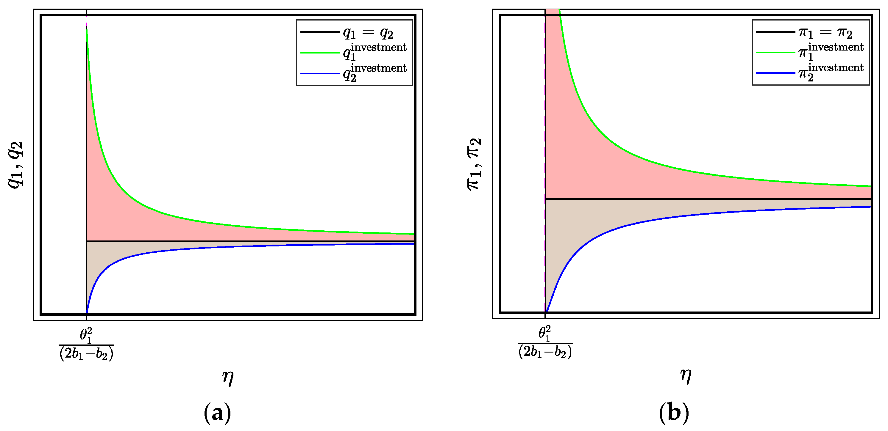
3.2. One Manufacturer Invests in Battery Life

Without loss of generality, we assume that one of the manufacturers invests in battery life technology, i.e., manufacturer 1 adopts the investment strategy, and we have $g_1>0$, $g_2=0$. Hence, the profits of the two manufacturers are given by:

$$\left\{\begin{array}{c}{\pi }_{m_1}=(a-b_1{q}_1-b_2{q}_2+\theta g_1-c_1)q_1-\frac{1}{2}\eta g_1^2\hfill \\ {\pi }_{m_2}=(a-b_1{q}_2-b_2{q}_1-c_2)q_2\hfill \end{array}\right.$$

(3)

In this model, the two manufacturers choose quantity and investment simultaneously and consider the other party’s decision. According to the first order condition, the best response functions are:

$$\left\{\begin{array}{c}{q}_1=\frac{a-c_1-b_2{q}_2+g_1\theta }{2b_1}\hfill \\ g_1=\frac{q_1\theta }{\eta }\hfill \\ q_2=\frac{a-c_2-b_2{q}_1}{2b_1}\hfill \end{array}\right.$$

(4)

Then, we find the equilibrium solution of model (3) is:

$$\begin{array}{cc}{E}^{*}\left(q_1,g_1,q_2\right)=\hfill & \left(\frac{(2a{b}_1-a{b}_2-2b_1{c}_1+b_2{c}_2)\eta }{4b_1^2\eta -b_2^2\eta -2b_1{\theta }^2},\right.\hfill \\ \hfill & \left.\frac{(2a{b}_1-a{b}_2-2b_1{c}_1+b_2{c}_2)\theta }{4b_1^2\eta -b_2^2\eta -2b_1{\theta }^2},\frac{(2a{b}_1-a{b}_2+b_2{c}_1-2b_1{c}_2)\eta +(-a+c_2){\theta }^2}{4b_1^2\eta -b_2^2\eta -2b_1{\theta }^2}\right)\hfill \end{array}$$

(5)

The profits of the two manufacturers are then as follows:

$$\left\{\begin{array}{c}{\pi }_1=\frac{{(2a{b}_1-a{b}_2-2b_1{c}_1+b_2{c}_2)}^2\eta (2b_1\eta -{\theta }^2)}{2{(-4b_1^2\eta +b_2^2\eta +2b_1{\theta }^2)}^2}\hfill \\ {\pi }_2=\frac{b_1{(b_2{c}_1\eta +a(2b_1\eta -b_2\eta -{\theta }^2)+c_2(-2b_1\eta +{\theta }^2))}^2}{{(-4b_1^2\eta +b_2^2\eta +2b_1{\theta }^2)}^2}\hfill \end{array}\right.$$

(6)

Proposition 1. 

To ensure the game system has the optimal solution and keep $q_i>0$,$g>0$,$\eta >\frac{{\theta }^2}{2b_1-b_2}$should be satisfied.

Proof. 

As described above, since the difference between the manufacturing costs of the two manufacturers is small, it can be considered $c_1=c_2$.

According to the profit function in Equation (3), one can find the Hessian matrix, and then we can discover that they are all concave functions so that there is an optimal solution when $\eta >\frac{{\theta }^2}{2b_1}$.

Additionally, since the manufacturer’s output and endurance levels should be positive, the following conditions also need to be met:

(1)

With $q_1>0$, we have

$\left\{\begin{array}{c}(2a{b}_1-a{b}_2-2b_1{c}_1+b_2{c}_2)\eta >0\hfill \\ 4b_1^2\eta -b_2^2\eta -2b_1{\theta }^2>0\hfill \end{array}\right.$ or $\left\{\begin{array}{c}(2a{b}_1-a{b}_2-2b_1{c}_1+b_2{c}_2)\eta <0\hfill \\ 4b_1^2\eta -b_2^2\eta -2b_1{\theta }^2<0\hfill \end{array}\right.$, as $2a{b}_1-a{b}_2-2b_1{c}_1+b_2{c}_2$ is greater than zero, so we have ${\eta }_1>\frac{2b_1{\theta }^2}{4b_1^2-b_2^2}$.

(2)

Based on (1), we know that $2a{b}_1-a{b}_2-2b_1{c}_1+b_2{c}_2$ is greater than zero, so $(2a{b}_1-a{b}_2-2b_1{c}_1+b_2{c}_2)\theta$ is greater than zero too, and $g_1$ greater than zero as well.

(3)

With $q_2>0$ we have

$\left\{\begin{array}{c}(2a{b}_1-a{b}_2+b_2{c}_1-2b_1{c}_2)\eta +(-a+c_2){\theta }^2>0\hfill \\ 4b_1^2\eta -b_2^2\eta -2b_1{\theta }^2>0\hfill \end{array}\right.$ or $\left\{\begin{array}{c}(2a{b}_1-a{b}_2+b_2{c}_1-2b_1{c}_2)\eta +(-a+c_2){\theta }^2<0\hfill \\ 4b_1^2\eta -b_2^2\eta -2b_1{\theta }^2<0\hfill \end{array}\right.$, as we know that ${\eta }_1>\frac{2b_1{\theta }^2}{4b_1^2-b_2^2}$, so we only need to find $(2a{b}_1-a{b}_2+b_2{c}_1-2b_1{c}_2)\eta +(-a+c_2){\theta }^2$ is positive, so we can obtain ${\eta }_2>\frac{{\theta }^2}{2b_1-b_2}$, as ${\eta }_2-{\eta }_1=\frac{b_2{\theta }^2}{4b_1^2-b_2^2}>0$, and so we finally have $\eta ={\eta }_2=\frac{{\theta }^2}{2b_1-b_2}$.

When $g_1=0$, and $\theta =0$, it means that manufacturer 1 has not adopted an investment strategy and the optimal strategies of the two manufacturers are the same. The corresponding equilibrium solution is:

$$E_{g=0}^{*}\left(q_1,g_1,q_2\right)=\left(\frac{2a{b}_1-a{b}_2-2b_1{c}_1+b_2{c}_2}{4b_1^2-b_2^2},\left.0,\frac{2a{b}_1-a{b}_2+b_2{c}_1-2b_1{c}_2}{4b_1^2-b_2^2}\right)\right.$$

(7)

The profits of the two manufacturers are as follows:

$$\left\{\begin{array}{c}{\pi }_1=\frac{b_1{(2a{b}_1-a{b}_2-2b_1{c}_1+b_2{c}_2)}^2}{{(-4b_1^2+b_2^2)}^2}\\ {\pi }_2=\frac{b_1{(2a{b}_1-a{b}_2-2b_1{c}_2+b_2{c}_1)}^2}{{(-4b_1^2+b_2^2)}^2}\end{array}\right.$$

(8)

In this case, the quantities and profits of the two manufacturers will be equal. As shown in Figure 2, the solid black line stands for the quantity and profit if neither of the two manufacturers invest in battery life technology. When one of the manufacturers adopts the investment strategy, its quantity and profit will change to the green line. The blue line represents the corresponding quantity and profit of the other manufacturer. □

Proposition 2. 

The quantity and profit of the manufacturer will increase if they adopt the investment strategy, and the quantity and profit of the other manufacturer who does not adopt the investment strategy will decrease when$\eta >\frac{{\theta }^2}{2b_1-b_2}$.

Proof. 

The proof is similar to Proposition 1 and is thus omitted. □

On the one hand, Proposition 2 shows that the manufacturer has the motivation to adopt an investment strategy to improve its profit, especially when the investment coefficient is small. That is to say, if the technology can be improved quickly through investment, it is beneficial to those enterprises with rapid response-ability, and some enterprises that are difficult to adapt to the market rhythm can be quickly eliminated. On the other hand, with the increase in the investment cost coefficient and the rise in the investment cost, more complicated phenomena may occur. From Figure 2, we know that as the cost factor of battery life investment increases, the quantities and profits of the two manufacturers will be the same. Combined with the difficulty and cycle of battery research and development, manufacturers may have insufficient incentives to invest, especially those with insufficient funds. However, enterprises with sufficient investment capabilities will still benefit from it.

4. Dynamic Game Model Analysis

The competition between manufacturers is very fierce. Therefore, once one manufacturer is in an advantageous position, he will maintain this advantage for some time, and another manufacturer will find them difficult to overtake quickly. Thus, the resulting optimal equilibrium solution is meaningful if one manufacturer adopts an investment strategy.

We can obtain the optimal equilibrium solution above through static model analysis which the manufacturers will use to make their decisions based on the equilibrium solution. Therefore, we present a repeated dynamic adjustment model in this section. To study the long-term game process of manufacturers, we assume that a limited rational approach will generally be adopted for the more forward-looking manufacturer when considering future development, and the short-sighted manufacturer will adopt adaptive expectations [34,35,36].

Then, the quantity decision of the two manufacturers at $t+1$ period can be described as follows. Among them, ${\alpha }_1$ represents the adjustment magnitude of one manufacturer’s output, ${\alpha }_2$ represents the adjustment range of their investment in battery life, and $v$ represents the adjustment speed of the other manufacturer’s production capacity.

$$\left\{\begin{array}{c}{q}_1(t+1)=q_1(t)+{\alpha }_1{q}_1(t)\frac{\partial {\pi }_1(q_1(t))}{\partial q_1(t)}\hfill \\ g_1(t+1)=g_1(t)+{\alpha }_2{g}_1(t)\frac{\partial {\pi }_1(g_1(t))}{\partial g_1(t)}\hfill \\ q_2(t+1)=(1-v)q_2(t)+v{q}_2(t)\frac{\partial {\pi }_2(q_2(t))}{\partial q_2(t)}\hfill \end{array}\right.$$

(9)

The stability and some of the complex phenomena of the dynamic game model will be analysed in the following subsection.

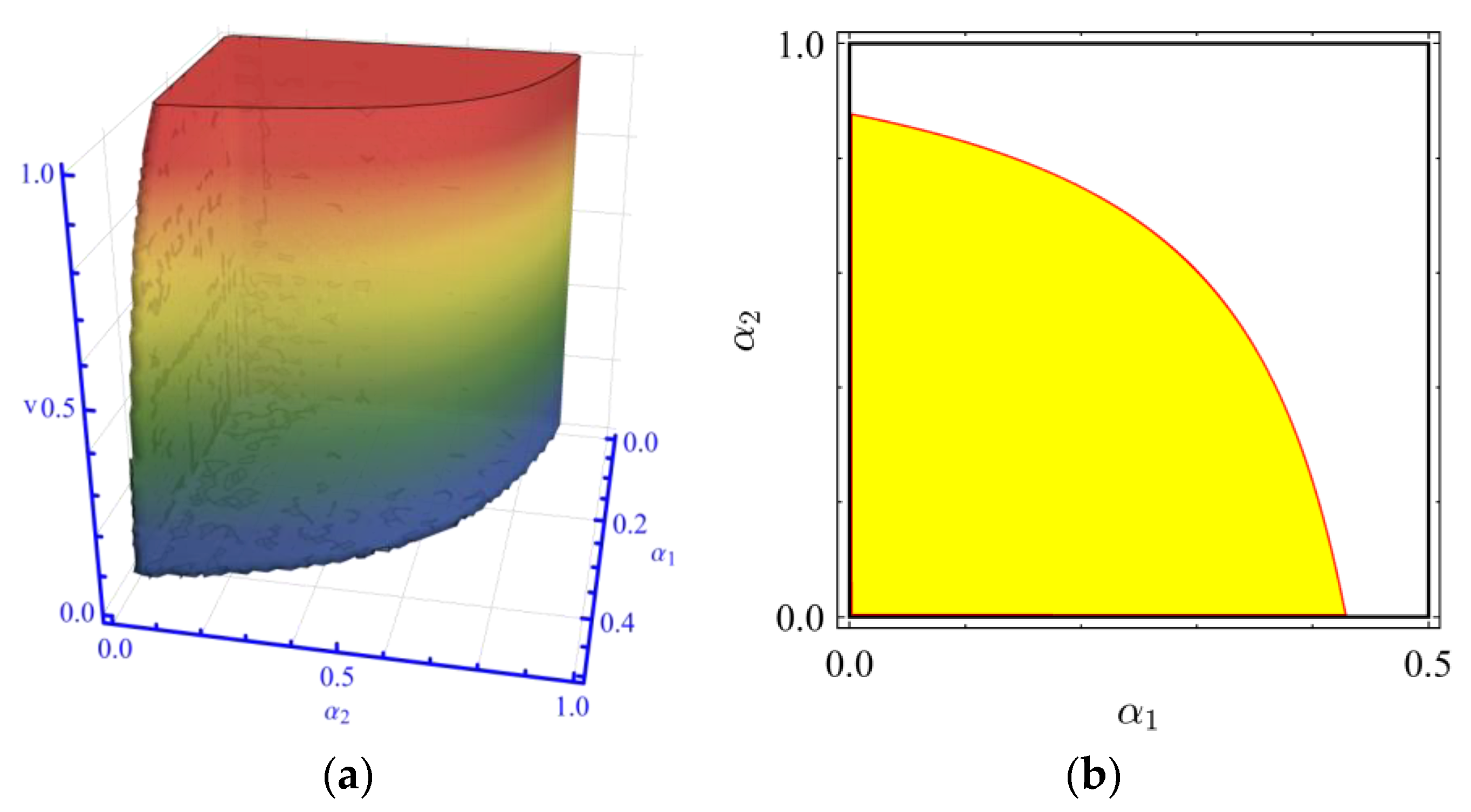
4.1. Equilibrium Points and Local Stability Analysis

A stable system is more conducive for decision-makers to judge and make decisions. In this subsection, we analyse the local stability of adversarial game systems. According to System (9), the equilibrium solution of the dynamic game system can be obtained. However, although the solution containing zero values is mathematically essential, it is not necessary for the manufacturer to consider the profit. Therefore, we only carry out the non-zero equilibrium solution here.

$$E^{*}\left(q_1,g_1,q_2\right)=\left\{\begin{array}{c}{q}_1=\frac{\left(2a{b}_1+b_2-a{b}_2-2b_1{c}_1+b_2{c}_2\right)\eta }{4b_1^2\eta -b_2^2\eta -2b_1{\theta }_{}^2}\hfill \\ g_1=\frac{\left(2a{b}_1+b_2-a{b}_2-2b_1{c}_1+b_2{c}_2\right){\theta }_{}}{4b_1^2\eta -b_2^2\eta -2b_1{\theta }_{}^2}\hfill \\ q_2=\frac{-2b_1\eta +2a{b}_1\eta -a{b}_2\eta +b_2{c}_1\eta -2b_1{c}_2\eta +{\theta }_{}^2-a{\theta }_{}^2+c_2{\theta }_{}^2}{4b_1^2\eta -b_2^2\eta -2b_1{\theta }_{}^2}\hfill \end{array}\right.$$

(10)

Then, we investigate the local stability of $E^{*}$ using the Jacobian Matrix of System (9). The Jacobian Matrix is:

$$\begin{array}{c}J=\left(\begin{array}{ccc}{j}_{11}\hfill & j_{12}\hfill & j_{13}\hfill \\ j_{21}\hfill & j_{22}\hfill & j_{23}\hfill \\ j_{31}\hfill & j_{32}\hfill & j_{33}\hfill \end{array}\right)\hfill \\ =\left(\begin{array}{ccc}1-2b_1{q}_1{\alpha }_1+{\alpha }_1\left(a-c_1-2b_1{q}_1-b_2{q}_2+g_1{\theta }_1\right)& q_1{\alpha }_1{\theta }_1& -b_2{q}_1{\alpha }_1\\ g_1{\alpha }_2{\theta }_1& 1-g_1{\alpha }_2\eta +{\alpha }_2\left(-g_1\eta +q_1{\theta }_1\right)& 0\\ -b_2{q}_{2}v& 0& 1-v-2b_1{q}_{2}v+\left(a-c_2-b_2{q}_1-2b_1{q}_2\right)v\end{array}\right)\hfill \end{array}$$

(11)

The Eigenvalues of $J$ are the solutions of the cubic equation of $\lambda$. As it is complicated, we give a brief expression here:

$$f\left(\lambda \right)={\lambda }^3+A{\lambda }^2+B\lambda +C=0$$

(12)

where $A$, $B$, and $C$ are the coefficients which are determined by $J$.

$$\left\{\begin{array}{c}A=\left(-j_{11}-j_{22}-j_{33}\right)\hfill \\ B=\left(-j_{12}{j}_{21}+j_{11}{j}_{22}-j_{13}{j}_{31}+j_{11}{j}_{33}+j_{22}{j}_{33}\right)\hfill \\ C=j_{13}{j}_{22}{j}_{31}+j_{12}{j}_{21}{j}_{33}-j_{11}{j}_{22}{j}_{33}\hfill \end{array}\right.$$

According to the Jury stability criterion, which gives a condition that all Eigenvalues must be inside the unit circle, the Nash equilibrium point is locally stable if the following four conditions are satisfied:

$$\left\{\begin{array}{c}{f}_1=f(1)=1+A+B+C>0\hfill \\ f_2={(-1)}^{3}f(-1)=-1+A-B+C>0\hfill \\ f_3=1-C^2>0\hfill \\ f_4={\left(1-C^2\right)}^2-{\left(B-AC\right)}^2>0\hfill \end{array}\right.$$

(13)

Based on Equation (13), we have:

$$\frac{{\left(2a{b}_1+b_2-a{b}_2-2b_{1}c+b_{2}c\right)}^{2}v{\alpha }_1{\alpha }_2\eta \theta \left(2b_1\left(-1+a-c\right)\eta +b_{2}c\eta +{\theta }^2+c{\theta }^2-a\left(b_2\eta +{\theta }^2\right)\right)}{{\left(-4b_1^2\eta +b_2^2\eta +2b_1{\theta }^2\right)}^2}>0$$

According to known conditions, we have: $\left(2b_1\left(-1+a-c\right)\eta +b_{2}c\eta +{\theta }^2+c{\theta }^2-a\left(b_2\eta +{\theta }^2\right)\right)>0$, so it will always be held, when $a>\frac{2b_1+2b_{1}c-b_{2}c}{2b_1-b_2}$ and $\eta >\frac{-{\theta }^2+a{\theta }^2-c{\theta }^2}{-2b_1+2a{b}_1-a{b}_2-2b_{1}c+b_{2}c}$.

The other three constraints are complex expressions containing three adjustment parameters; it is very difficult to obtain the analytical solution directly, so we mainly combine the numerical simulation in the following analysis.

Since the theoretical results are complex and inconvenient to observe, we combine the numerical simulation to give a graphical illustration to satisfy the constraints. Based on the constraint conditions of the parameters in the above propositions, the parameter values that satisfy the conditions can be given as $a=5, b_1=1.6, b_2=1.1, c_1=0.8, c_2=0.8, \theta =1.6,\mathrm{and} \eta =4$. As shown in Figure 3, according to the Jury stability condition in Equation (13), we can find the stable region in the three-dimensional space of the adjustment parameters.

Figure 3a shows the stable region in the three-dimensional space of $\left({\alpha }_1,{\alpha }_2,v\right)$, it can be seen that there are many fine black lines on the surface of the stable region, which intersect with the definition domain and indicate that the boundary surface is not smooth, which also shows the complexity of the stability domain. Figure 3 also indicates that the system will remain stable only when the parameters are in this region. For a more intuitive understanding, we perform dimensionality reduction processing. As shown in Figure 3b, i.e., $g=0.5$, the stable region is shown by the yellow colour.

There are many complex features and phenomena in System (9) that should be attended to and investigated. For example, when the adjustment parameters change, the manufacturer’s decision will also change, and after a certain period, it may enter a bifurcation or a chaotic state. At this time, the decision-makers need to pay more attention to the long-term evolution process of the game system. As shown in Figure 4, ${\alpha }_1$ represents the adjustment of production by manufacturer 1. Assuming that ${\alpha }_2$ and $v$ are fixed, we can observe the impact of ${\alpha }_1$ on system stability. As shown in Figure 4a, when the adjustment speed ${\alpha }_1$ is less than a certain critical value, the system is in a stable state and there is an equilibrium solution. When ${\alpha }_1$ is greater than a certain critical value, the system will enter a bifurcated state, and as ${\alpha }_1$ continues to increase, the system will enter a chaotic state. Correspondingly, the state change of the system can be observed more intuitively through the largest Lyapunov exponent graph in Figure 4b. The Lyapunov exponent reflects the distance between iterative motion trajectories. If the Lyapunov exponent is less than zero, it indicates that the motion trajectory exhibits a contraction trend as the number of iterations increases. Conversely, it indicates that the iteration trajectory tends to diverge. The part less than zero corresponds to the stable range of the system and the part greater than zero corresponds to the unstable range of the system.

Figure 4 indicates that when the decision-makers make decisions, it is necessary to consider the value range of the parameter and the impact of parameter changes on the system entirely. Otherwise, it will make the system unstable or uncontrollable. Parameters such as ${\alpha }_2$ and $v$ have similar properties; the bifurcation and the largest Lyapunov exponents are shown in Figure 5 and Figure 6, respectively.

Decision-makers do not want the system to enter a bifurcated or chaotic state because it will make it difficult for decision-makers to predict and control the system. Therefore, the decision-maker will want to control the value of the tuning parameter within a stable range.

With the change of the adjustment parameters, the system will experience period-doubling bifurcation, from a stable state to an unstable state. As shown in Figure 7a, we can observe that the yellow region is stable. When the parameters stay in the yellow region, the system only has a single-cycle solution and indicates a steady state. Different colours indicate other periods. For example, the orange region is the cycle of period 2; the light blue region is the cycle of period 4; the light blue region is the cycle of period 8, and so on. The crimson region is for chaos, and the dark blue region is for divergence. Figure 7b,c has a similar meaning, where Figure 7d shows the corresponding periodic slices in three-dimensional space. The colours in Figure 7d represent the same system status as above.

To observe the impact of the adjustment parameters on System (9), Figure 8 shows the influence of the two-parameter change on the system’s stability, periodicity, and chaotic state in the two-dimensional plane.

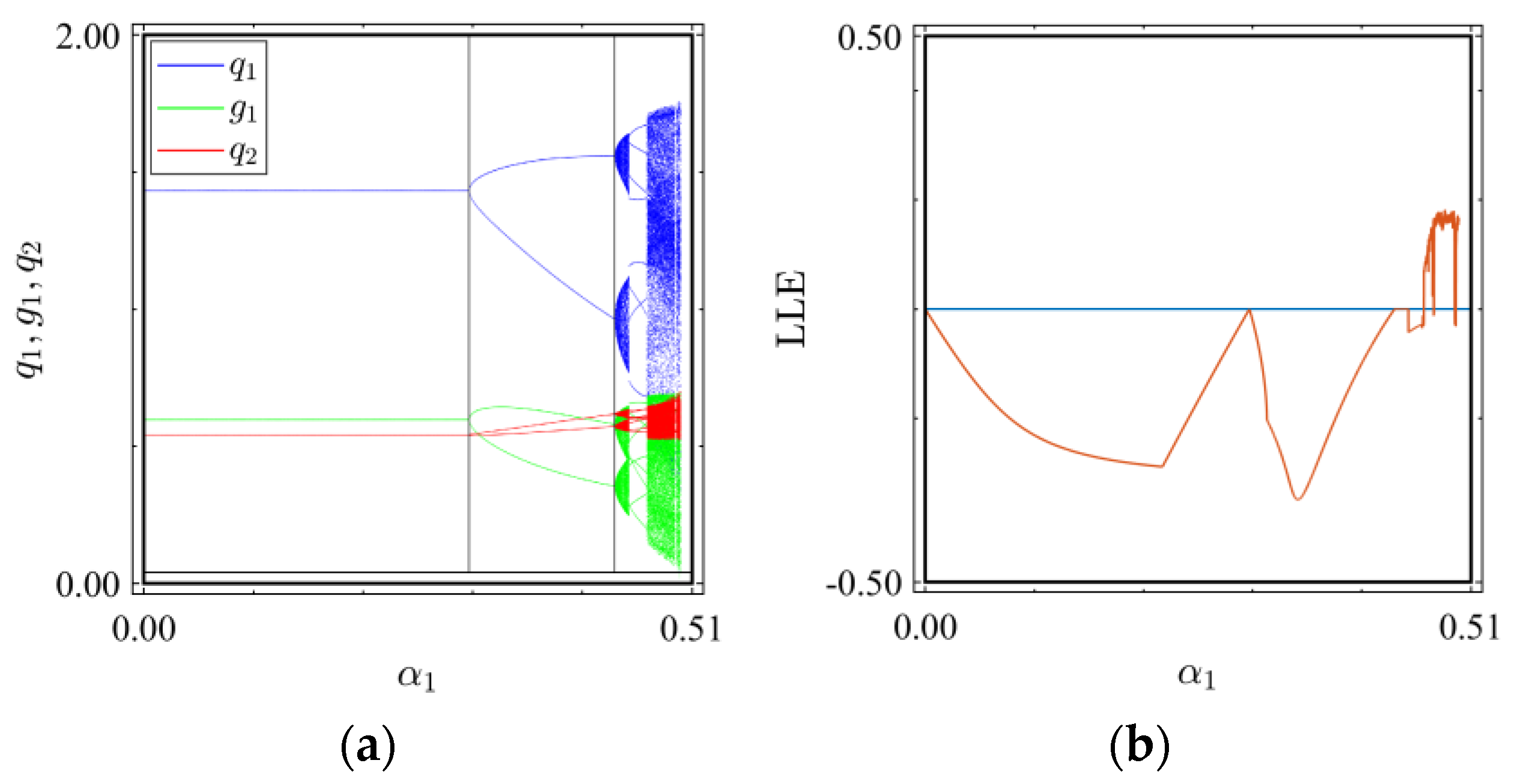
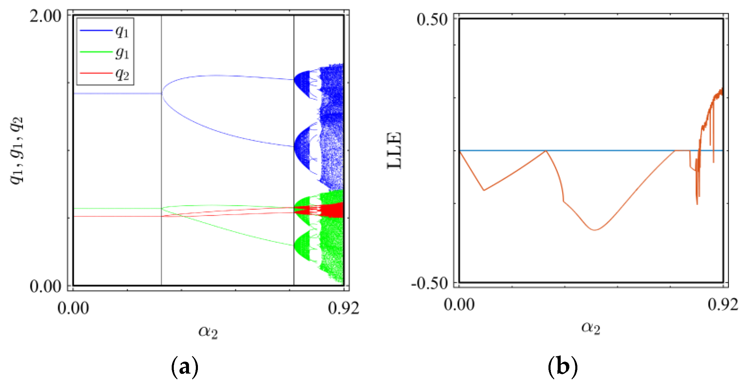
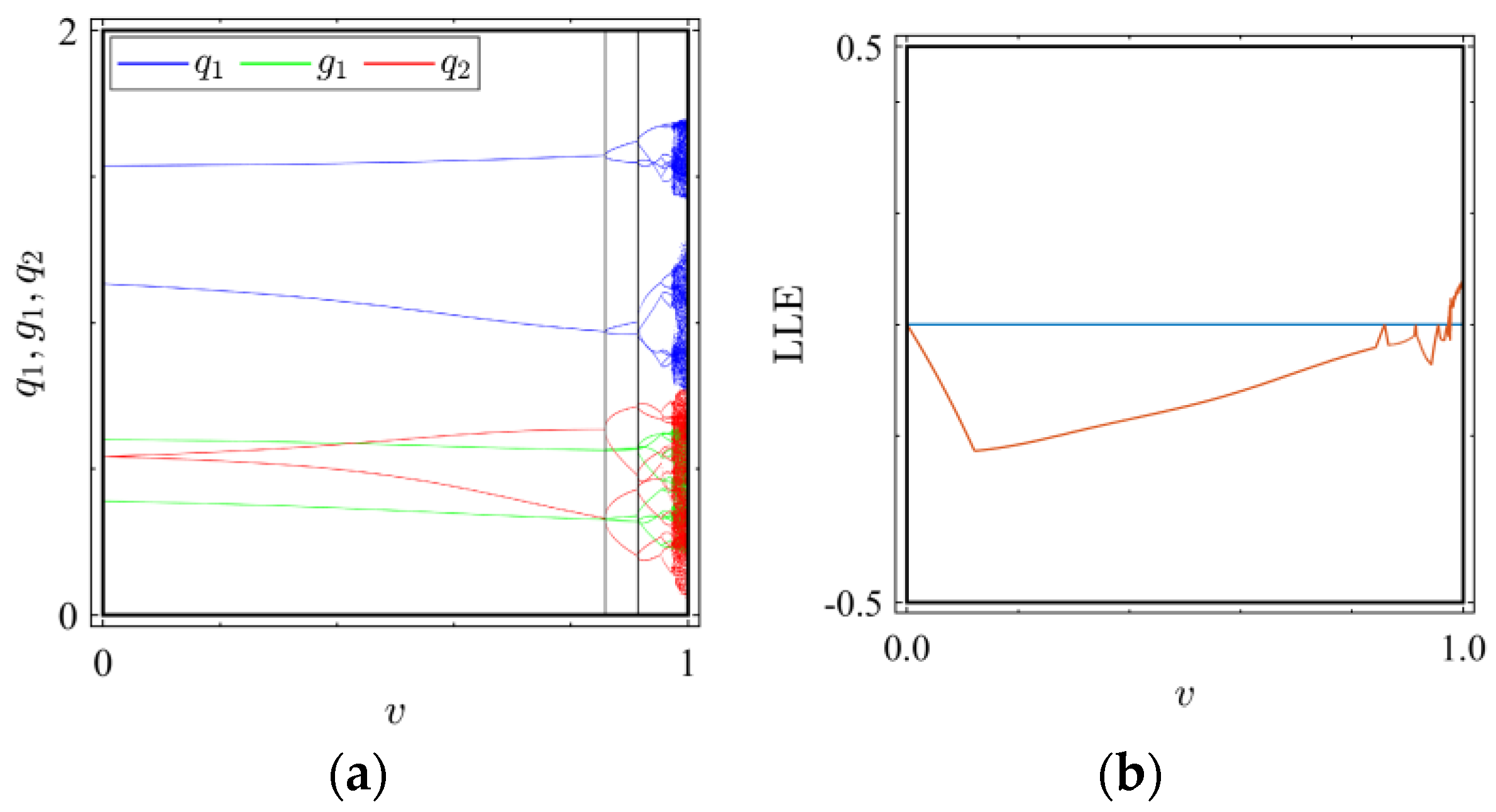
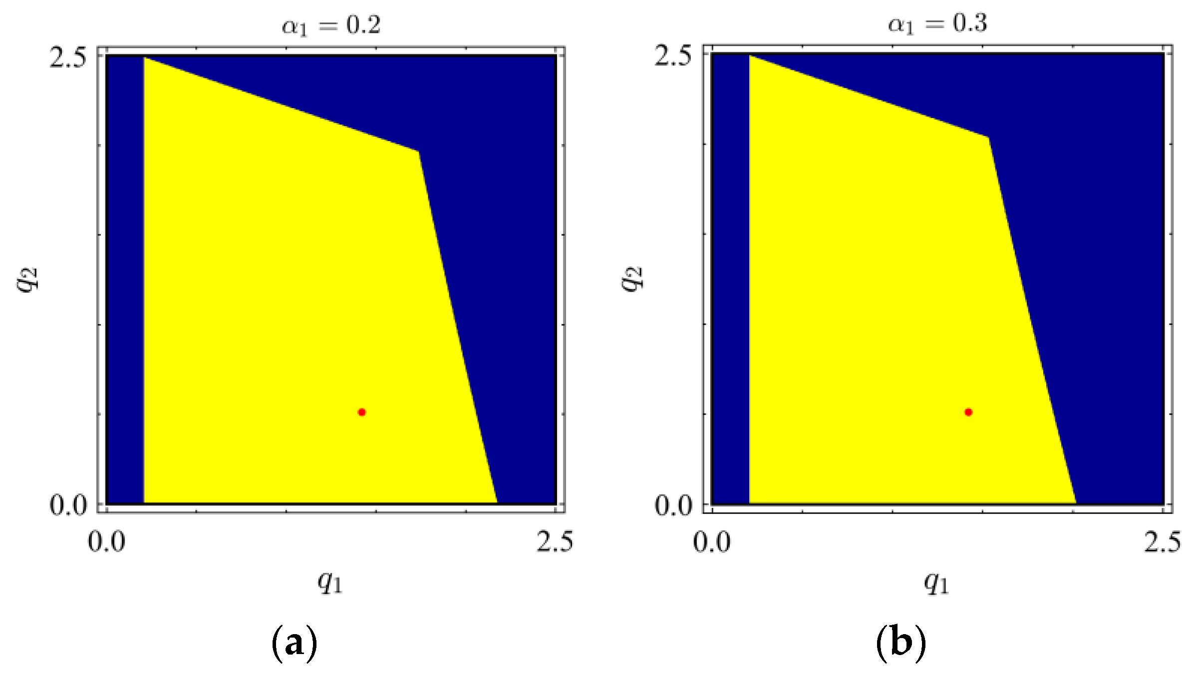
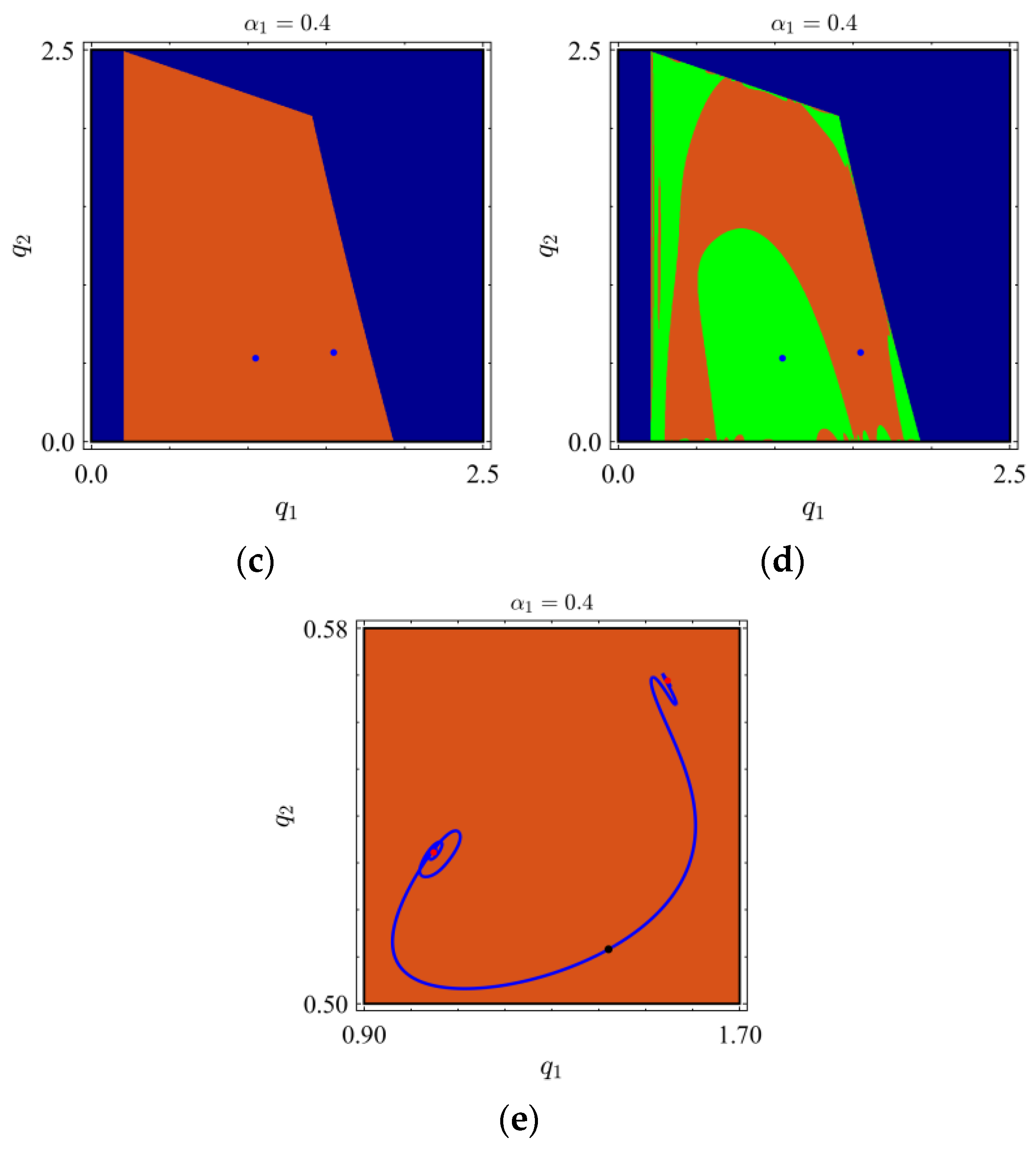
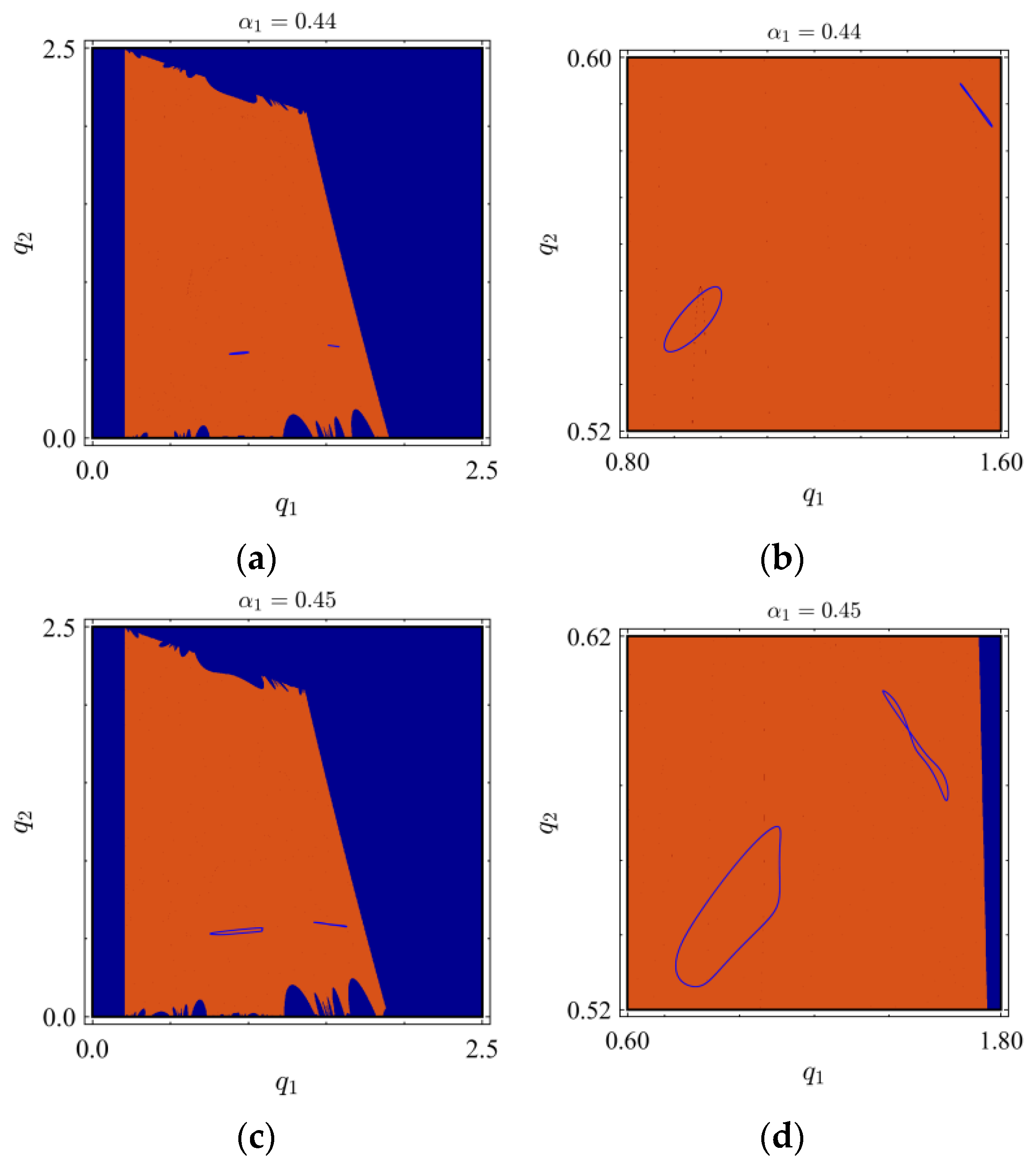
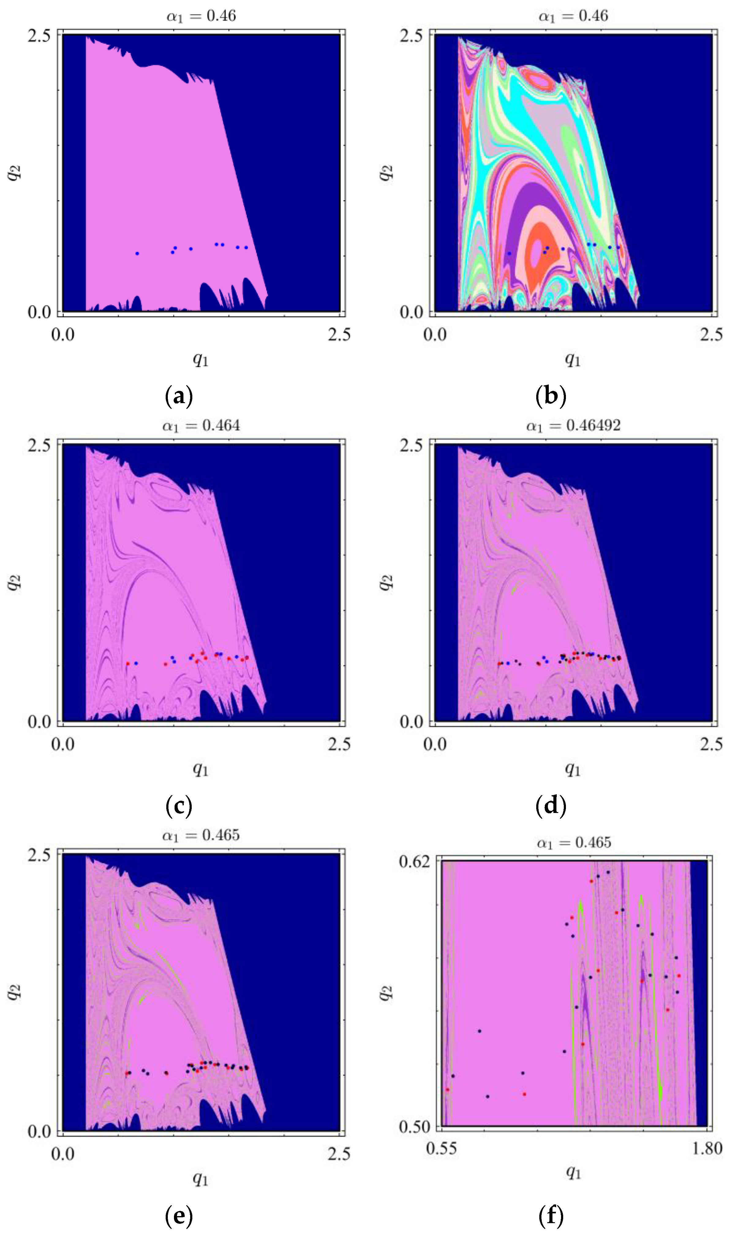
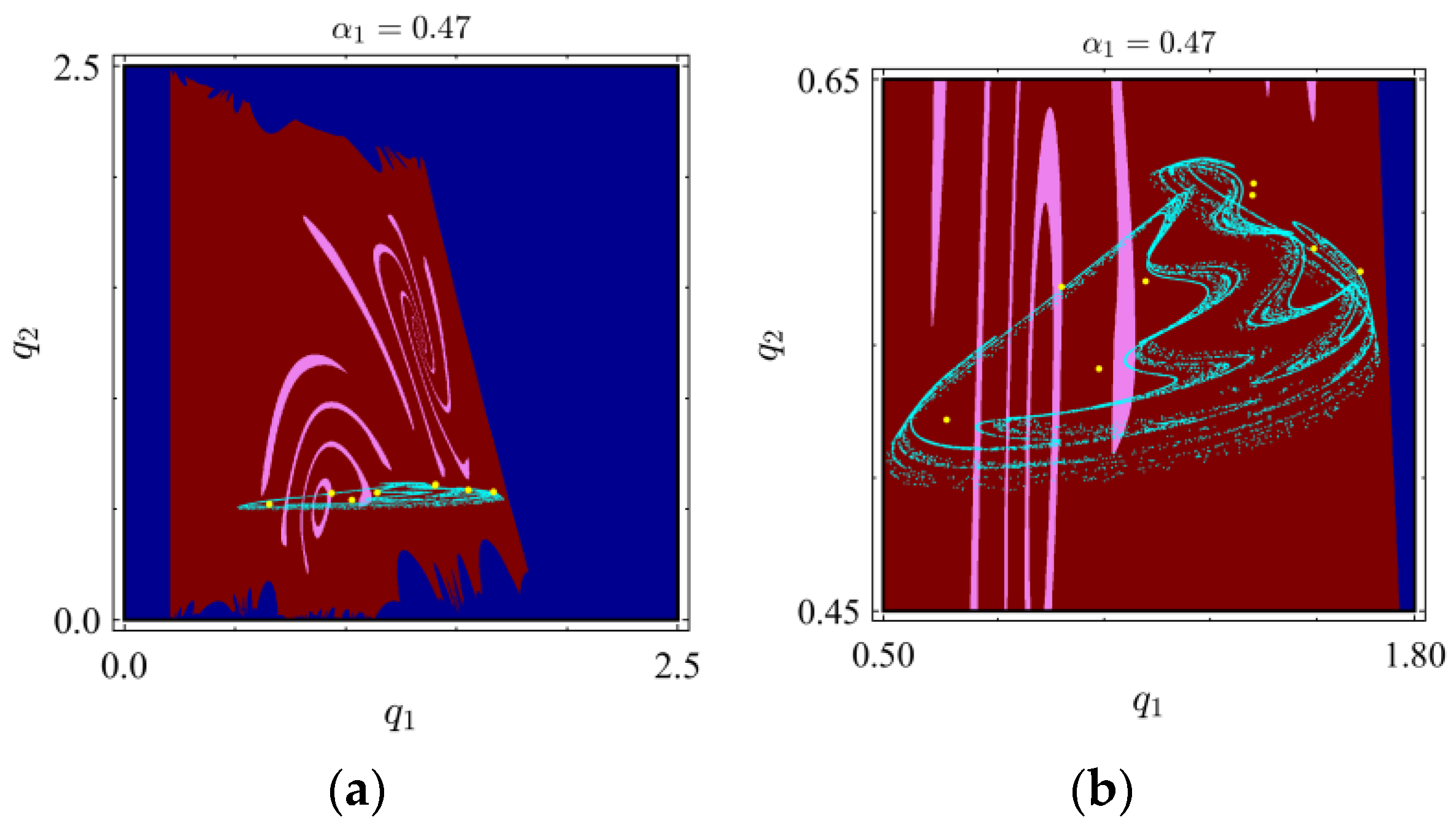
4.2. Global Bifurcation and Attractors

The basins of attraction correspond to the set of initial conditions whose long-time response (LTR) approaches the attractor. Based on this concept, we change the initial conditions to study the effect of different initial values on the system’s attractor. The coexistence of several attractors exists widely in nonlinear systems, which increases the complexity and difficulty of analysis. In this paper, the discrete dynamical systems have several attractors too.

With the varying of parameter ${\alpha }_1$, the basins of attraction will also change. As shown in Figure 8, there are a series of basins of attraction in the $\left(q_1,q_2\right)$ plane. In Figure 8a,b, the initial values in the yellow region will converge to a red fixed point, but we find that the stable region in Figure 8b is smaller. As shown in Figure 8c, as parameter ${\alpha }_1$ increases, only one red fixed point changes to two blue fixed points, and the basin of attraction becomes smaller. Figure 8d shows the different converge domains using two colours, and Figure 8e presents the trajectory from the stable point (black) to the two fixed points (red).

With the further increase in parameters, the system will develop more complex characteristics and phenomena. As shown in Figure 9, there are two invariant curve cycles, that is, the two blue cycles in the orange area. Figure 9a,c contains the entire basins of attraction and Figure 9b,d shows the enlarged figures.

The decision-makers may be confused when the emergence of invariant curve cycles leads to constant changes in the optimal solution. However, fortunately, invariant curve cycles are still within the predictable range.

When the parameters are near the critical value of bifurcation, the phenomenon of coexisting attractors will occur. Since multiple solutions exist simultaneously, it may disturb the decision result, which is very unfavourable for the decision-maker. Figure 10a presents the basins of attraction of cycles of period 8, and they are marked by different colours in Figure 10b. Then, we continue to increase the value of ${\alpha }_1$; Figure 10c–e presents the coexisting attractors. At this time, 8-period and 10-period solutions will appear simultaneously.

In Figure 10e, there are three coexisting attractors. As shown in Figure 10f, we can clearly distinguish the number of cycles. It shows the cycles of period 8, cycles of period 10, and cycles of period 18 attractors. The initial values in the pink region will converge to cycles of period 8, the initial values in the orchid region will converge to cycles of period 10, and the initial values in the chartreuse region will converge to cycles of period 18. It also shows the complexity of the dynamic System (9) and indicates that the choice of the initial value will significantly influence the decision result.

With the further increase in the parameters, the coexistence of the eight-period attractor and chaotic attractor will appear in the dynamic System (9), which will seriously disturb the decision-making behaviour of the manufacturer. For example, when ${\alpha }_1=0.47$, there is a stable cycle of period 8 and a chaos attractor. Figure 11a,b shows this phenomenon. The teal area in Figure 11 represents a chaotic attractor.

Combining the system’s attractors can allow for a better observation and discussion of the change of the dynamic system state with the parameter change. Figure 12 shows the attractors in the $\left(q_1,g_1,q_2\right)$-space. As shown in Figure 12, there are six types of attractors present, they are the 1-period, 2-period, two invariant curve cycle, 166-period, 8-period, and chaos attractor.

In this subsection, through the study of the basins of attraction and attractors, we find that the complex system will gradually enter a chaotic state as the parameters change and that the initial state is important for decision-makers. When other parameters change, similar phenomena will also occur, which undoubtedly dramatically increases the difficulty of the decision-making process. If it cannot be predicted in advance, it will have a significant impact on the future development of the enterprise.

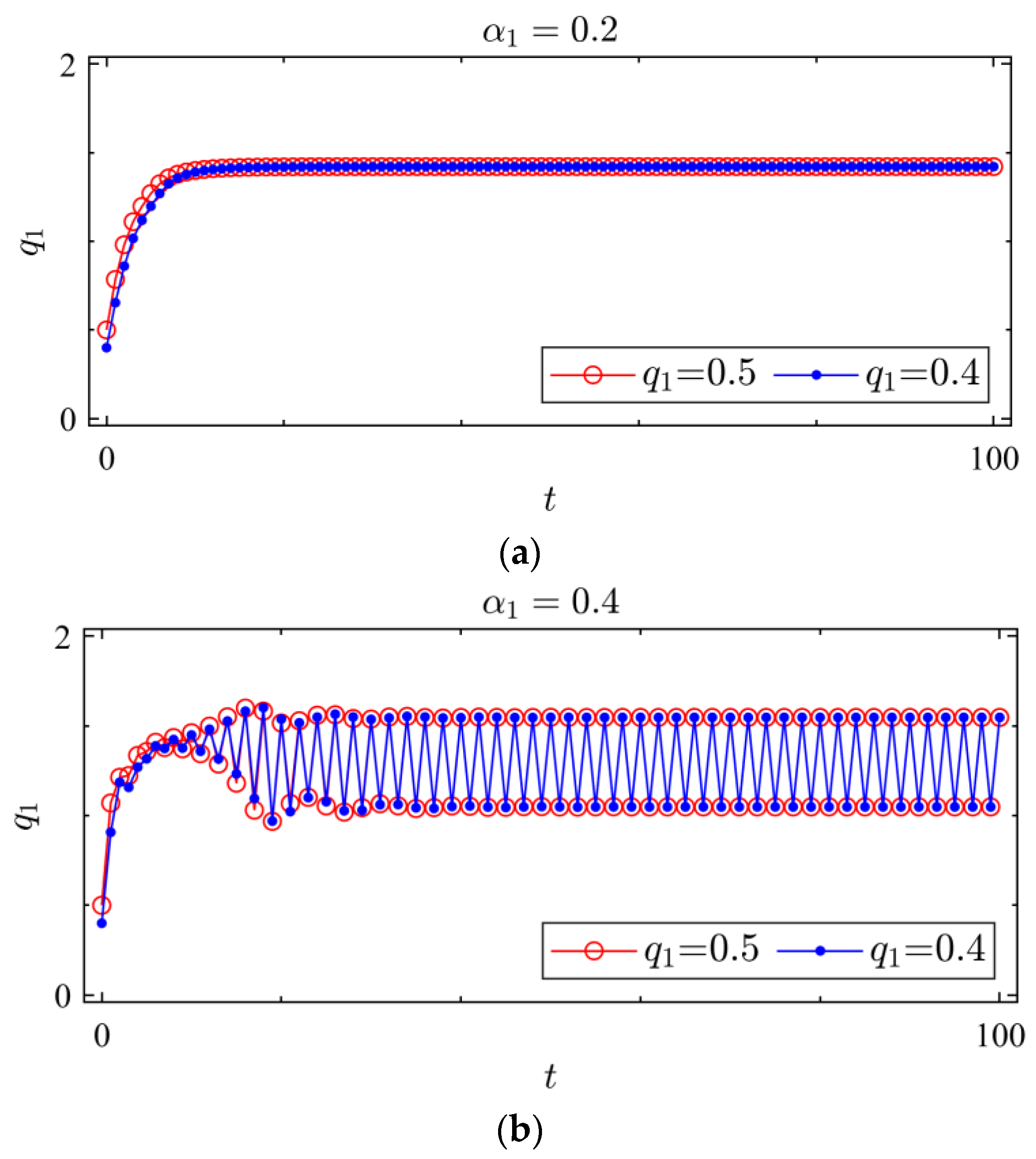
4.3. Sensitivity Analysis

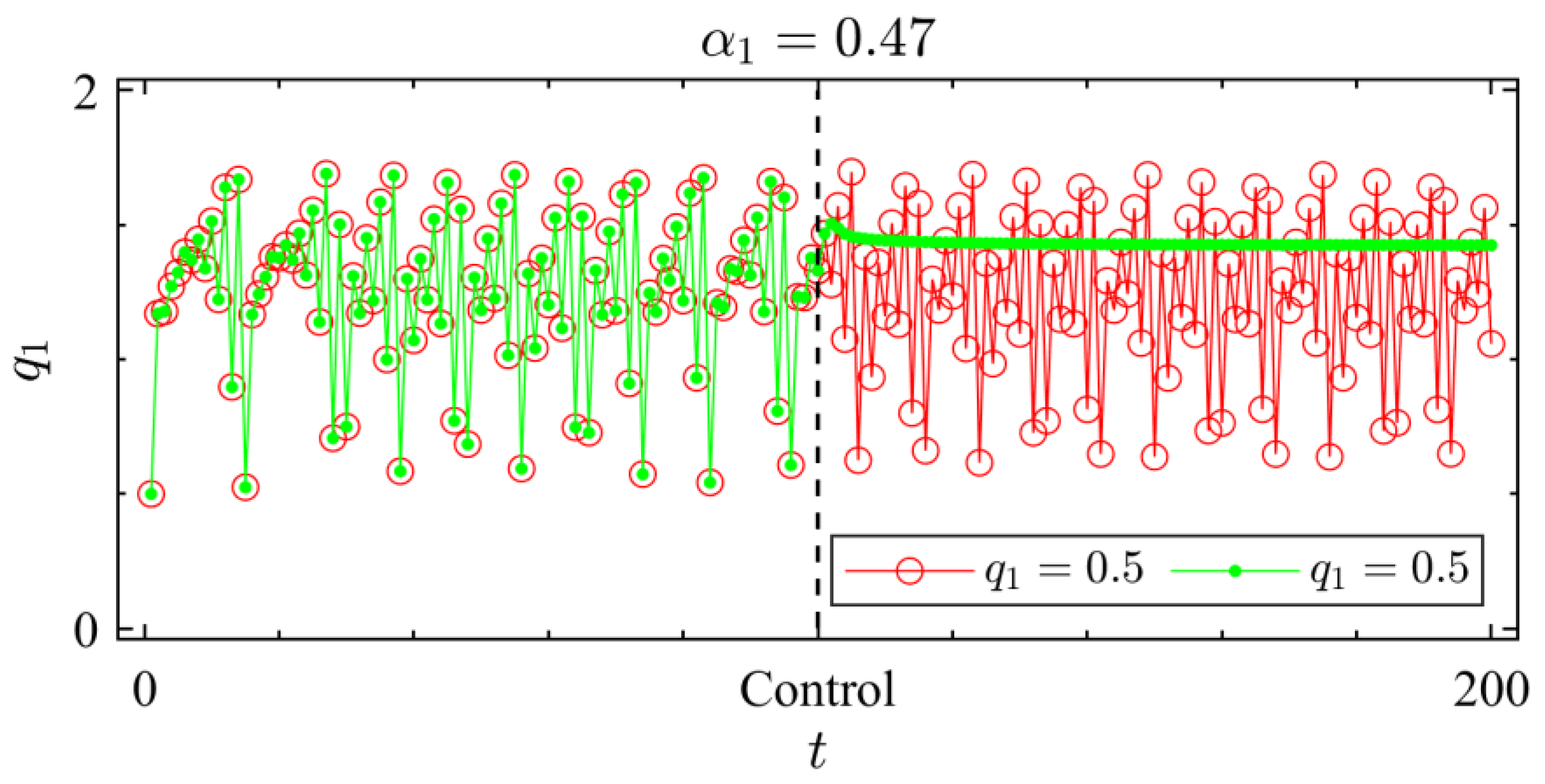
As initial value sensitivity is one of the important features of a chaotic system, the state changes of complex dynamic systems can also be observed and analysed through the time series. For example, Figure 13 shows the time series graph under different values of ${\alpha }_1$.

Figure 13a–c shows the time series diagram after assigning different initial values to $q_1$ after 100 iterations. It can be found that although the initial value is different, they can stabilise to the same fixed points after several iterations. Figure 13a shows that the system maintains a stable single-period solution after several iterations, while Figure 13b presents a two-period and Figure 13c presents an eight-period.

Although the two sequences in Figure 13c do not look the same, the same periodic solution can be obtained after adjusting the sequence’s order. As shown in Figure 14, the blue point set only needs to be translated five to the right to coincide with the red point set.

As shown in Figure 15, although the initial value difference is slight when the dynamic system enters the chaotic state, the result will significantly differ after several iterations. Similarly, there are similar situations for other adjustment parameters. In a chaotic state, the decision-making results are difficult to predict, which will bring great difficulties to decision-makers. However, chaos is unavoidable in many cases. Therefore, it is necessary to find an effective control method to intervene so that the game system can recover to a stable state.

4.4. Chaos Control

Through the given constraints and actual conditions, decision-makers can generally determine the range of each parameter. However, as analysed above, chaotic phenomena may occur inadvertently. Therefore, at this time, decision-makers need to master effective chaos control methods to keep the dynamic system in a stable state.

In this subsection, we introduce the OGY control method to deal with chaos. We know that when ${\alpha }_1=0.47$ the system will go into chaos. Therefore, to verify the method’s effectiveness, we control the chaos system after 100 iterations. As shown in Figure 16, the red points stand for the chaos times series and the green points stand for the times series after control. The black dashed line is the control time point.

From Figure 16, we know that the dynamic system returns to a stable state when we adopt the chaos control method. This is undoubtedly desirable to decision-makers who can control the system within a controllable range through effective control methods, thereby minimising uncertainty.

5. Conclusions

In this paper, we examined the issue of electric vehicle manufacturers investing in battery life and modelled and analysed this issue in combination with duopoly electric vehicle manufacturers in the market. It can be found that when the investment coefficient is low, the return on R&D investment is relatively high. On the other hand, as the investment coefficient increases, its profit will gradually decrease, and it will be close to the case of no investment. At this time, enterprises may choose not to invest but purchase related technologies after the technologies are mature.

We also studied the complex phenomenon and mechanism produced by the enterprise’s long-term game decision-making by combining complex dynamic game theory. In the long-period dynamic game process, the decision-making result of the enterprise is closely related to the decision-making coefficient. With the change of the adjustment parameters, bifurcation and chaos may appear in the system, and there may be period-doubling bifurcation and N-S bifurcation at the same time, which increases the difficulty of decision-making. From the perspective of global bifurcation, it can be found that the system’s initial state will also change the system’s stability and even create the coexisting attractor phenomenon.

Through the analysis of the game, we found many interesting conclusions. First, electric vehicle manufacturers’ investment in batteries is related to investment costs. If the investment cost is high, manufacturers will have a lower investment incentive. In contrast, if the investment cost is low, it will promote the manufacturer’s investment enthusiasm. The government should help electric vehicle manufacturers reduce investment costs, encourage financial institutions to provide low interest rate loans to electric vehicle manufacturers, and support the integration of industry, academia, and research. Manufacturers should also strive to develop and improve battery life. Secondly, through the analysis of the long-period dynamic game, it can be found that the manufacturer’s decision is closely related to the system parameters. Subtle changes in parameters may lead to disorder of the game system and or even cause it to enter a chaotic state through periodic bifurcation and N-S bifurcation. The choice of the initial state also has an important impact on the game results. Different basins of attraction will lead to the emergence of varying solution sets and even the phenomenon of coexisting attractors. It undoubtedly increases the difficulty of decision-making for decision-makers, so decision-makers may prefer to maintain the system in a stable state. We found that the chaotic control method can be used to restore the chaotic system to a steady state.

In summary, this paper can provide theoretical support and decision-making suggestions for decision-makers through the study of the electric vehicle manufacturer investing in battery life. Therefore, it has research and management significance. In future research work, we will further combine the investment decision-making issues of electric vehicle manufacturers under the influence of policies and compare and study purchasing or leasing technology content. In addition, the energy conversion efficiency of electric vehicle batteries and the time-sharing pricing mechanism of charging stations can also be discussed in the future.

References

1. Ma, J.; Hou, Y.; Wang, Z.; Yang, W. Pricing strategy and coordination of automobile manufacturers based on government intervention and carbon emission reduction. Energy Policy 2021, 148, 111919. [Google Scholar] [CrossRef]
2. Ma, J.; Hou, Y.; Yang, W.; Tian, Y. A time-based pricing game in a competitive vehicle market regarding the intervention of carbon emission reduction. Energy Policy 2020, 142, 111440. [Google Scholar] [CrossRef]
3. Ma, J.; Si, F.; Zhang, Q.; Huijiang. Evolution delayed decision game based on carbon emission and capacity sharing in the Chinese market. Int. J. Prod. Res. 2022. [Google Scholar] [CrossRef]
4. Ma, J.; Xu, T. Optimal Strategy of Investing in Solar Energy for Meeting the Renewable Portfolio Standard Re-quirement. J. Oper. Res. Soc. 2022, 74, 181–194. [Google Scholar] [CrossRef]
5. Ma, J.; Zhu, L.; Guo, Y. Strategies and stability study for a triopoly game considering product recovery based on closed loop supply chain. Oper. Res. 2021, 21, 2261–2282. [Google Scholar] [CrossRef]
6. Binshuo, B.; Junhai, M.; Mark, G. Short- and long-term repeated game behaviours of two parallel supply chains based on government subsidy in the vehicle market. Int. J. Prod. Res. 2020, 58, 7507–7530. [Google Scholar]
7. Xu, T.; Ma, J. Feed-in tariff or tax-rebate regulation? Dynamic decision model for the solar photovoltaic supply chain. Appl. Math. Model. 2021, 89, 1106–1123. [Google Scholar] [CrossRef]
8. Ma, J.; Xie, L. The stability analysis of the dynamic pricing strategy for bundling goods: A comparison between simulta-neous and sequential pricing mechanism. Nonlinear Dyn. 2019, 95, 1147–1164. [Google Scholar] [CrossRef]
9. Zhu, Y.; Xia, C.; Chen, Z. Nash Equilibrium in Iterated Multiplayer Games Under Asynchronous Best-Response Dynamics. IEEE Trans. Autom. Control. 2023. [Google Scholar] [CrossRef]
10. Ma, J. Nonlinear Analysis Methods for Complex Economic and Financial Systems; Beijing Science Press: Beijing, China, 2021; Volume 6. [Google Scholar]
11. Dong, C.; Liu, Q.; Shen, B. To be or not to be green? Strategic investment for green product development in a supply chain. Transp. Res. Part E Logist. Transp. Rev. 2019, 131, 193–227. [Google Scholar] [CrossRef]
12. Zheng, Y.; Zhang, G.; Zhang, W. A Duopoly Manufacturers’ Game Model Considering Green Technology Investment under a Cap-and-Trade System. Sustainability 2018, 10, 705. [Google Scholar] [CrossRef]
13. Sun, H.; Wan, Y.; Zhang, L.; Zhou, Z. Evolutionary game of the green investment in a two-echelon supply chain under a government subsidy mechanism. J. Clean. Prod. 2019, 235, 1315–1326. [Google Scholar] [CrossRef]
14. Li, Z.; Pan, Y.; Yang, W.; Ma, J.; Zhou, M. Effects of government subsidies on green technology investment and green mar-keting coordination of supply chain under the cap-and-trade mechanism. Energy Econ. 2021, 101, 105426. [Google Scholar] [CrossRef]
15. Liu, L.; Wang, Z.; Zhang, Z. Matching-Game Approach for Green Technology Investment Strategies in a Supply Chain under Environmental Regulations. Sustain. Prod. Consum. 2021, 28, 371–390. [Google Scholar] [CrossRef]
16. Li, C.; Liu, Q.; Zhou, P.; Huang, H. Optimal innovation investment: The role of subsidy schemes and supply chain channel power structure. Comput. Ind. Eng. 2021, 157, 107291. [Google Scholar] [CrossRef]
17. Li, Z.; Yang, W.; Liu, X.; Taimoor, H. Coordination strategies in dual-channel supply chain considering innovation investment and different game ability. Kybernetes 2020, 49, 1581–1603. [Google Scholar] [CrossRef]
18. Zhang, L.; Wang, J.; You, J. Consumer environmental awareness and channel coordination with two substitutable products. Eur. J. Oper. Res. 2015, 241, 63–73. [Google Scholar] [CrossRef]
19. Hong, Z.; Wang, H.; Yu, Y. Green product pricing with non-green product reference. Transp. Res. Part E Logist. Transp. Rev. 2018, 115, 1–15. [Google Scholar] [CrossRef]
20. Chen, J.-Y.; Dimitrov, S.; Pun, H. The impact of government subsidy on supply Chains’ sustainability innovation. Omega 2019, 86, 42–58. [Google Scholar] [CrossRef]
21. Ueda, M. Effect of information asymmetry in Cournot duopoly game with bounded rationality. Appl. Math. Comput. 2019, 362, 124535. [Google Scholar] [CrossRef]
22. Yang, X.; Peng, Y.; Xiao, Y.; Wu, X. Nonlinear dynamics of a duopoly Stackelberg game with marginal costs. Chaos Solitons Fractals 2019, 123, 185–191. [Google Scholar] [CrossRef]
23. Lou, W.; Ma, J. Complexity of sales effort and carbon emission reduction effort in a two-parallel household appliance supply chain model. Appl. Math. Model. 2018, 64, 398–425. [Google Scholar] [CrossRef]
24. Elsadany, A.A.; Awad, A.M. Dynamics and chaos control of a duopolistic Bertrand competitions under environmental taxes. Ann. Oper. Res. 2019, 274, 211–240. [Google Scholar] [CrossRef]
25. Zhou, J.; Zhou, W.; Chu, T.; Chang, Y.-X.; Huang, M.-J. Bifurcation, intermittent chaos and multi-stability in a two-stage Cournot game with R&D spillover and product differentiation. Appl. Math. Comput. 2019, 341, 358–378. [Google Scholar] [CrossRef]
26. Askar, S.; Al-Khedhairi, A. Dynamic investigations in a duopoly game with price competition based on relative profit and profit maximization. J. Comput. Appl. Math. 2020, 367, 112464. [Google Scholar] [CrossRef]
27. Wu, F.; Ma, J. The equilibrium, complexity analysis and control in epiphytic supply chain with product horizontal diversification. Nonlinear Dyn. 2018, 93, 2145–2158. [Google Scholar] [CrossRef]
28. Wang, H.; Ma, J. Complexity analysis of a Cournot–Bertrand duopoly game with different expectations. Nonlinear Dyn. 2014, 78, 2759–2768. [Google Scholar] [CrossRef]
29. Ma, J.; Sun, L. Complex dynamics of a MC–MS pricing model for a risk-averse supply chain with after-sale investment. Commun. Nonlinear Sci. Numer. Simul. 2015, 26, 108–122. [Google Scholar] [CrossRef]
30. Nobakhti, E.; Khaki-Sedigh, A.; Vasegh, N. Control of Multichaotic Systems Using the Extended OGY Method. Int. J. Bifurc. Chaos 2015, 25, 1550096. [Google Scholar] [CrossRef]
31. Chen, D.; Ignatius, J.; Sun, D.; Zhan, S.-L.; Zhou, C.; Marra, M.; Demirbag, M. Reverse logistics pricing strategy for a green supply chain: A view of customers’ environmental awareness. Int. J. Prod. Econ. 2019, 217, 197–210. [Google Scholar] [CrossRef]
32. Martín-Herrán, G.; Sigué, S.P. An integrative framework of cooperative advertising: Should manufacturers continuously support retailer advertising? J. Bus. Res. 2017, 70, 67–73. [Google Scholar] [CrossRef]
33. Martín-Herrán, G.; Sigué, S.P. Retailer and manufacturer advertising scheduling in a marketing channel. J. Bus. Res. 2017, 78, 93–100. [Google Scholar] [CrossRef]
34. Ma, J.; Sun, L. Complexity analysis about nonlinear mixed oligopolies game based on production cooperation. IEEE Trans. Control. Syst. Technol. 2018, 26, 1532–1539. [Google Scholar] [CrossRef]
35. Zhu, Y.; Zhang, Z.; Xia, C.; Chen, Z. Equilibrium analysis and incentive-based control of the anticoordinating networked game dynamics. Automatica 2023, 147, 110707. [Google Scholar] [CrossRef]
36. Zhu, Y.; Xia, C.-Y.; Wang, Z.; Chen, Z. Networked Decision-Making Dynamics Based on Fair, Extortionate and Generous Strategies in Iterated Public Goods Games. IEEE Trans. Netw. Sci. Eng. 2022, 9, 2450–2462. [Google Scholar] [CrossRef]
Figure 1. Supply chain structural framework.
Mathematics 11 03551 g001
Figure 2. Comparison of quantities and profits. (a) The impact of investment coefficient on quantity, (b) The impact of investment coefficient on profits.
Mathematics 11 03551 g002
Figure 3. (a) The stable region in the α 1 , α 2 , v -space; (b) The stable region in the α 1 , α 2 -plane.
Mathematics 11 03551 g003
Figure 4. (a) Bifurcation diagram of System (9) when α 1 0 , 0.51 and (b) the largest Lyapunov exponents corresponding to (a).
Mathematics 11 03551 g004
Figure 5. (a) Bifurcation diagram of System (9) when α 2 0 , 0.92 and (b) the largest Lyapunov exponents corresponding to (a).
Mathematics 11 03551 g005
Figure 6. (a) Bifurcation diagram of System (9) when v 0 , 1 and (b) the largest Lyapunov exponents corresponding to (a).
Mathematics 11 03551 g006
Figure 7. (a) Two-dimensional bifurcation diagram in the α 1 , α 2 plane; (b) two-dimensional bifurcation diagram in the α 1 , v plane; (c) two-dimensional bifurcation diagram in the α 2 , v plane; and (d) three-dimensional periodic slice diagram in the α 1 , α 2 , v space.
Mathematics 11 03551 g007
Figure 8. Basins of attraction and attractors. (a) The basin of attraction with α 1 = 0.2 ; (b) the basin of attraction with α 1 = 0.3 ; (c) the basin of attraction with α 1 = 0.4 ; and (d) the basin of attraction with α 1 = 0.4 , showing two focus points with two colours. (e) The trajectory of stable points to unstable points.
Mathematics 11 03551 g008aMathematics 11 03551 g008b
Figure 9. Basins of attraction and attractors. (a) The basin of attraction with α 1 = 0.44 ; (b) the basin of attraction with α 1 = 0.44 and an enlarged axis; (c) the basin of attraction with α 1 = 0.45 ; and (d) the basin of attraction with α 1 = 0.45 and an enlarged axis.
Mathematics 11 03551 g009
Figure 10. (a) The basin of attraction with α 1 = 0.46 ; (b) the basin of attraction with α 1 = 0.46 and labelled by different colours; (c) the basin of attraction with α 1 = 0.464 ; (d) the basin of attraction with α 1 = 0.46492 ; (e) the basin of attraction with α 1 = 0.45 ; and (f) the basin of attraction with α 1 = 0.465 and an enlarged axis.
Mathematics 11 03551 g010
Figure 11. Basins of attraction and attractors. (a) The basin of attraction with α 1 = 0.47 and (b) the basin of attraction with α 1 = 0.4745 and figure enlargement.
Mathematics 11 03551 g011
Figure 12. Attractors with α 1 varying. (a) α 1 = 0.2 ; (b) α 1 = 0.4 ; (c) α 1 = 0.45 ; (d) α 1 = 0.45154 ; (e) α 1 = 0.464 ; and (f) α 1 = 0.7 .
Mathematics 11 03551 g012aMathematics 11 03551 g012b
Figure 13. Time series of q 1 with α 1 varying. (a) α 1 = 0.2 ; (b) α 1 = 0.4 ; and (c) α 1 = 0.46 .
Mathematics 11 03551 g013aMathematics 11 03551 g013b
Figure 14. Time series of q 1 with α 1 = 0.46 in a 3-D view.
Mathematics 11 03551 g014
Figure 15. Time series of q 1 with α 1 = 0.47 .
Mathematics 11 03551 g015
Figure 16. Chaos control after 100 iterations with α 1 = 0.47 .
Mathematics 11 03551 g016